Conference paper

(1)

AUTOMATIC SURFACE CLASSIFICATION FOR RETRIEVING AREAS WHICH ARE

HIGHLY ENDANGERED BY EXTREME RAIN

Peter Fischera ∗

, Thomas Kraußa_{, Dr. Tim Peters}b

a

Remote Sensing Technology Institute, German Aerospace Center (DLR), M¨unchener Str. 20, 82234 Wessling, Germany -(Peter.Fischer, Thomas.Krauss)@dlr.de

b

Westf¨alische Provinzial Versicherung AG, Provinzial-Allee 1, 48181 M¨unster - Tim.Peters@provinzial.de

Commission VII, WG VII/4

KEY WORDS:Automatic DSM classification, Terrain Positioning Index, extreme rain, damage probability

ABSTRACT:

In this case study, an approach for finding regions endangered by extreme rain is presented. The approach is based on the assumption that sinks in the surface are more endangered than their surroundings. The surface data, which are the source for the classification, are generated using a Cartosat stereo scene. The classification is performed by using an algorithm for retrieving the terrain positioning index. Different classification schemes are possible, therefore a set of input parameters is iteratively computed. The classification results are then evaluated. For validating the classification stock data of an insurance are used. We compare the position of the reported damages caused by extreme rain with our classification. By doing so we got the confirmation of the assumption.

1. INTRODUCTION

Human made objects face in general several types of dangers, which are related to small scale weather events, like storms, vol-ley and extreme rain. The orography of a location strongly deter-mines the influence of an extreme weather event on the human entities placed at the location. Finding indexes for spatial re-gions based on the orography which indicate the probability of being affected by an extreme weather event is therefore essential. Such indexes would enable decision makers to develop strategies where structures like roads, bridges and settlements can be placed with an minimal risk of being damaged by extreme weather phe-nomena.

There has been a lot of work done in the field of automated ter-rain classification. A broad range of indexes and classification algorithms is already developed, which take the presence of dis-crete regions like watersheds (Tagil and Jenness, 2008), or re-gions which can be described as geomorphological enclosed ar-eas (Reu et al., 2013). These indexes describe the surface as is. This serves as entry point to our application, where we investigate the influence of orography to the relationship between extreme weather events and the probability of damage to human entities located on earth surface. This is a quite complex task, due to the differing dependencies of spatial exposition and damage event for various weather events. For example a short distance to a river may be a good indicator for a high risk of floods, but for a storm event the influence is probably negligible. We want to show the impact of the spatial exposition of entities on the probability of being affected by extreme rain events.

Insurance companies already have zoning systems which classify the risk of locations being affected by extreme rain and flooding. These existing systems work quite well for floods. But analysis of damage and stock data have shown that for backwater and ex-treme rain existing zoning systems don’t deliver reliable results. This can be explained by the methodology used for zoning the space . In general the systems take the euclidean distance to the

∗_{Corresponding author.} _{Tel.: +49 8153 281561; fax: +49 8153} 281444.

next streaming water body into account. By doing so, in case of an flooding event which affects this water body for every point on the surface an estimation can be made about the probability of being affected by this flooding.

Extreme rain events in contrast are not bounded to streaming wa-ter bodies. They occur at almost every place on earth surface, and the risk of a damage on the ground is mainly related to the exposition of a body on the ground. In this paper we prove the assumption that sinks on the surface are higher endangered than hilltops. This assumption is based on the nature of fluids to follow the gradient of surfaces to minimize their potential.

2. DATA BASE 2.1 Digital Elevation Model

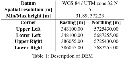
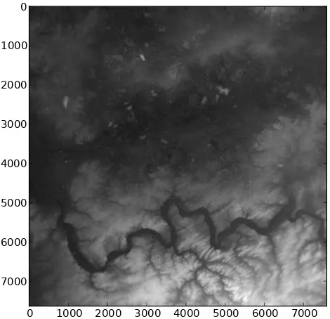
As source data for the classification algorithm a digital elevation model retrieved from an Cartosat stereo scene is used, which is shown in figure 1. The parameters describing the spatial extent, resolution and the projection of the DEM are listed in table 1.

Datum WGS 84 / UTM zone 32 N Spatial resolution [m] 5

Min/Max height [m] 31.89, 372.23 Corner Easting [m] Northing [m] Upper Left 348100.00 5725430.00 Lower Left 348100.00 5687255.00 Upper Right 386055.00 5725430.00 Lower Right 386055.00 5687255.00

Table 1: Description of DEM

(2)

0 1000 2000 3000 4000 5000 6000 7000 0

1000

2000

3000

4000

5000

6000

7000

Figure 1: Digital Elevation Model

Furthermore we took an digital terrain model aquired by the Shut-tle Radar Topography Mission (Farr et al., 2007), to compare the influence of spatial resolution but moreover the influence of different acquisition systems. By doing so, we can determine whether surface models retrieved by radar systems deliver at least comparable results to models retrieved from optical systems.

2.2 Geocoded insurance data

The data provided by the insurance are divided into stock data and damage event data, where only damage events caused by ex-treme rain were taken into account. The stock data contain infor-mation about all households who own an elementary insurance for extreme rain, the damage dataset lists households who were affected by an damage event in the time span from 2003 to 2013.

The stock data table has five attributes, which are described in table 2. Each dataset represents a household which is specified by an unique insurance number, 3D coordinates (UTM), the in-sured sum and auxiliary data. The stock data table contains 24997 households which own an elementary insurance.

attribute type meaning

VSNR int unique insurance id, primary key

x double easting [m]

y double northing [m]

z double height [m]

vers summe int insurance sum [e]

Table 2: Description of Stock Data attributes

The damage data table has six attributes, three for the location of the damage, one for the contract id, one for the costs of the damage and one for the date when a damage occurred. Table 3 gives an overview of the attributes. The number of households which were affected by a damage is 735.

Figure 2 depict the distribution of the households in the test area. Cyan dots mark households which own an insurance, red dots mark the households which were affected by an damage event.

attribute type meaning

SCHDAT date date of damage

VSNR int unique insurance id, primary key auf String costs (’aufwand’) [e]

x double easting [m]

y double northing [m]

z double height [m]

Table 3: Description of Damage Data attributes

Figure 2: Distribution of households in test areal

3. TERRAIN CLASSIFICATION ALGORITHM 3.1 Theoretical Background

The TPI (1) is the basis of a classification system and is simply the difference between a cell elevation valuez0 and the average elevationzof the neighbourhoodRaround the cell (Weiss, 2001) (Wilson and Gallant, 2000).

T P I=z0−z (1)

z= 1

nR

X

i∈R

zi (2)

There are two situations for a kernel map moving over a surface, which can be distinguished easily. On the one side the height value at a point pt is greater than the mean elevationµ in the neighbourhood of this point. Therefor the TPI value is also pos-itive. On the other side the mean elevationµis greater than the elevation at point pt, because of this the TPI value is lower than zero.

To distinguish between flat areas and points on slopes, the slope angles, described in (Zevenbergen and Thorne, 1987) are also taken into account. Such situations occur for example at hillside situations. For computing the slope angles, the following equa-tions 3 and 4 are used.

sx,y=

s

∆z

∆x 2

+

∆z

∆y 2

(3)

s◦x,y =

arctan(sx,y)

π∗180 (4)

In the project the DEV index is used which is based on the TPI. DEV (5) measures the topographic position as a fraction of local relief normalised to local surface roughness (Reu et al., 2013), the equations are given in 5 and 6.

DEV =z0−z

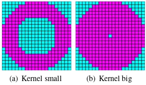
The main influencing factor of the TPI and DEV value are the two parameters inner radius and outer radius, which define the resulting kernel map. In figure 3 two different kernel maps are shown. For both kernel maps, the outer radius is 10 pixels. For figure 3(a), the inner radius is 5 pixel, for figure 3(b) the inner radius is zero pixels. Thus the resulting number of height values taken into account is for the small kernel 252 in contrast to 348 height valus for the big kernel map.

(a) Kernel small (b) Kernel big

Figure 3: Comparison of different kernel sizes

Depending on the kernel size the classified result can diver quite much. If a small kernel map is used for classifying a DSM, small landforms can be distinguished in the resulting classification. If the same DSM is classified using a bigger kernel map, which is done by using a bigger outer radius, then the small landforms become generalized. The resulting output image therefore gives more small scale landforms. Finding the right kernel size is an it-erative process, depending on the application (Tagil and Jenness, 2008).

The classification schema itself remains the same for different kernel maps, in most cases the one given in table 4 is used. This classification schema gives 6 classes, as input a DEV image and a slope image is needed. It is also possible to combine different kernel maps and therefor to gain more sophisticated classes.

Naming class DEV Slope

Table 4: Classification rules - 6 classes, adapted from (Jenness, 2006)

Subsequent an overview of different classifications is shown. The goal is to show the influence of different inner and outer radii on the resulting classification. For outer and inner radius, the three tupels [300,100] m,[600,200]m and[900,300]m are used. Like already in section 2.1 mentioned, we also want to analye the in-fluence of different spatial resolutions of the input DSM on the

classification results. Grohmann (Grohmann et al., 2009) already showed that for surface roughness the influence of the spatial res-olution can be neglected to some extent. To get a first clue, the source DSM with five metres resolution and a downsampled ver-sion with 20 metres resolution is used. Figure 4 shows the classi-fication results based on the original DSM with five metres spa-tial resolution. In figure 4(a) as algorithm parameters the radii tupel[300,100]m is used, this means the kernel is specified with an outer radius of 300 metres and an inner radius of 100 metres. With increasing radii in figure 4(b) and figure 4(c) the scale of the landforms classified decreases. Especially the river network gets very general in figure 4(c). The colour legend is given in table 4(g).

The same classifications were done on the downsampled DSM with an spatial resolution of 20 metres, the results are depicted in figure 4(d), 4(e) and 4(f) respectively. Compared to the classi-fication results gained with the high resolution DSM, almost no difference can be detected visually. This supports the observa-tions done by (Grohmann et al., 2009).

3.2 Proposed Algorithm

This classification algorithm is implemented as XDibias (Triendl et al., 1982) modul using Python (G. van Rossum and F.L. Drake, 2001) and Cython (Behnel et al., 2011) programming language. The idea of the algorithm consists of three steps.

1. The classification algorithm is applied to the three source DSMs with different combinations for the two parameters specifying the kernel map, inner and outer radius.

2. The classified raster dataset is merged with the point data from the insurance, for each single point in the two datasets the corresponding class is stored. Therefore a script based on the PointSampling Tool from Quantum GIS (QGIS De-velopment Team, 2009) is implemented.

3. An grading matrix is computed to compare the classifica-tion results. The hypothesis is that households in valleys are more probable affected by damages than households on hilltops. This means the probability of being affected by an damage based on extreme rain should be higher for house-holds in valleys. The structure of such a grading matrix is described in detail in the following.

The grading matrix, shown in equation 7, consists of the results from the mentioned three steps. There are 6 rows, which corre-spond to the total number of land form classes. The first column gives the name of the classax, for examplea1is valley. Second and third column give the total distribution of householdsbxwith

contract and of damaged householdscx. Column four and five

give the total costs for each classdxand the total insured sum for

each classexin euro. Column six gives the claims ratefxfor

each class, which is computed with equation 8. Column seven gives the number of damaged householdsgxin percent per class,

which is computed with equation 9 .

(4)

(a) TPI, 300 100, retrived from original DSM (b) TPI, 600 200, retrived from original DSM (c) TPI, 900 300, retrived from original DSM

(d) TPI, 300 100, retrived from or DSM (e) TPI, 600 200 (f) TPI, 900 300

class valley lower slope flat mid slope upper slope hilltop color

(g) Color legend

Figure 4: Comparison classification results for different kernel masks and spatial resolutions of DSM

g[%] =cx

bx

∗100 (9)

4. RESULTS AND DISCUSSION

Four DSMs were processed, having a spacial resolution of 5,10 and 20 and 66 meters respectively. The parameter for the inner kernel radius ranges from 50 to 700 meters with a step length of 50 meters, the parameter for the outer radius ranges from 100 to 900 meters, step length is also 50 meters. This leads to 441 classified images for each of the four DSMs, all of them linked to a grading matrix.

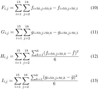
The main objective is to answer the question, whether house-holds in depressions are more affected by extreme rain, and if yes, which kernel radii fit best for the land form classification. To answer both questions, four descriptors are computed for the different surface models and the different radii combinations, and then stored in the four matrixesF, G, H, I.

1. The difference between class one and six for the claim rate, computed with equation 10.

2. The difference between the percentage of affected house-holds for class one and six, computed with equation 11.

3. The variance in the claim rates over the six classes, see equa-tion 12.

4. The variance in the percentage of affected households over the six classes, see equation 13.

Fi,j=

15 X

i=1 18 X

j=2

fi∗50,j∗50,6−fi∗50,j∗50,1 (10)

Gi,j=

15 X

i=1 18 X

j=2

gi∗50,j∗50,6−gi∗50,j∗50,1 (11)

Hi,j=

15 X

i=1 18 X

j=2 P6

k=1(fi∗50,j∗50,k−f¯) 2

6 (12)

Ii,j=

15 X

i=1 18 X

j=2 P6

k=1(gi∗50,j∗50,k−¯g) 2

6 (13)

(5)

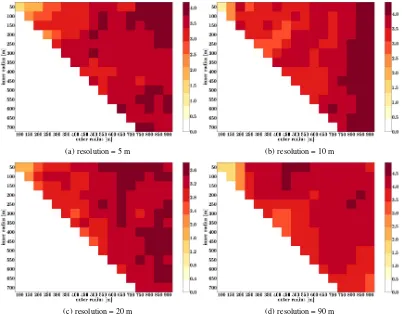
difference. The claim rate differences resulting from the process-ing with SRTM data are smallest, not reachprocess-ing values higher than 7. In Figure 6 a detailed view is given for the variance in the claim rates. It is shown that the variance reaches also it’s maximum val-ues when using the Cartosat data downsampled with factor two.

The same evaluation was made for the damage probabilities, fig-ure 7 depicts the difference between the number of affected house-holds per class [%] in class one and class six. Figure 8 shows the variance in the single number of affected households per class [%].

We see that the observation from the claim rates is somehow mir-rored into this plots. Also for the probabilities a big outer radius and a small inner radius seems to be a good advice. And also here, the influence of the spatial resolution of the input DSM seems al-most negligible for the Cartosat DSMs. Probably the point that the downsampled DSM with 10 m spatial resolution delivers the best results can be explained when taking into account, that veg-etation and other error sources for land form classification are filtered by the downsampling. On the other hand taking the radar data from SRTM does not deliver that good results, probably be-cause of the lower spatial resolution. Furthermore when it comes to find the maximum difference for the number of affected house-holds between hilltops and valley, a small outer radius of 450 m and an inner radius of 50 m seems to deliver also reliable results.

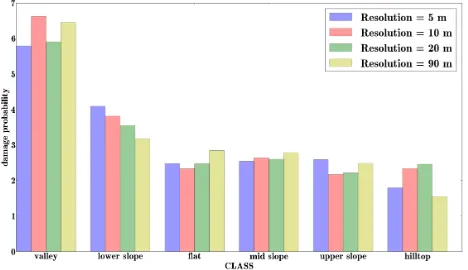
Exemplary we compare the classification result retrieved with us-ing 900 meters as outer radius and 150 meters as inner radius for optical data and 450 meters as outer radius and 50 meters as inner radius for SRTM data. These combinations give us the most promising results in the previous investigations. Figure 7(a) shows the decrease of the percentage of affected households from the valley to the hilltop. This trend is shown, no matter whether the classification is based on optical or radar data. In the claim rates this trend is depicted even stronger. This means that not just more households in valleys are affected by extreme rain than on hilltops, but also that the costs of the single damages are in general higher in valleys.

Figure 9: Percentage of affected households per class

5. CONCLUSIONS AND FUTURE WORK By combining the outcomes from claim rate differences and claim rate variance, we come to the conclusion that big outer radii in general suite best for reaching good classification results. The in-ner radius in contrast should be quite small, not bigger than 300 meters. An outer radius of 900 meters and an inner radius of 150 meters seem to deliver the most satisfying results for high resolu-tion optical data. The influence of the spatial resoluresolu-tion is at least not that big - this can be explained with keeping in mind that the

Figure 10: Claims Rate for different resolutions

lower resolution DSMs are retrieved by downsampling the high resolution DSM using linear interpolation.

For low resolution radar data the inner radius was taken as low as possible, the outer radius was not bigger than 450 m. More investigations should be done on the influence of the different data record methods, here radar and optical systems. For example the degree of soil moisture and vegetation cover at record time have different influences on the resulting surface model - which influences the land form classification.

The results showed that the spatial exposition of houses has great on the claim rate and probability of the occurence of an damage caused by extreme rain. By using more sophisticated algorithms for land form classification and taking more spatial descriptors like curvature and land cover into account, probably the model could be even more accurate.

ACKNOWLEDGEMENTS

This project is funded by the department of Technology Market-ing of German Aerospace Center, and carried out in a strategic in-novation partnership with Westf¨alische Provinzial Versicherung Aktiengesellschaft, Germany. The authors gratefully acknowl-edge the support and assistance of Robert Klarner, DLR TM RBO OP. Furthermore the authors would like to thank Frank Bistrick and Roman Kolbe from Westf¨alische Provinzial Versicherung for the initial stock and damage data and discussions.

REFERENCES

Behnel, S., Bradshaw, R., Citro, C., Dalcin, L., Seljebotn, D. and Smith, K., 2011. Cython: The best of both worlds. Computing in Science Engineering 13(2), pp. 31 –39.

Farr, T., Rosen, P., Caro, E., Crippen, R., Riley, D., Hensley, S., Kobrick, M., Paller, M., Rodriguez, E., Roth, L., Seal, D., Shaf-fer, S., Shimada, J., Umland, J., Werenr, M., Oskin, M., Burbank, D. and Alsdorf, D., 2007. The shuttle radar topography mission. Reviews of Geophysics.

G. van Rossum and F.L. Drake, 2001. Python Reference Manual. PythonLabs, Virginia, USA.

Grohmann, C., Smith, M. and Riccomini, C., 2009. Surface roughness of topography: A multi-scale analysis of landform ele-ments in midland valley, scotland. Proceedings of Geomorphom-etry 2009 pp. 140–148.

(6)

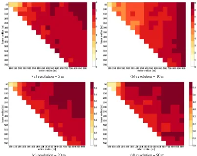
(a) resolution = 5 m (b) resolution = 10 m

(c) resolution = 20 m (d) resolution = 90 m

Figure 5: Claim Rate Difference Class 1 - Class 6 for different resolutions

Jones, E., Oliphant, T., Peterson, P. et al., 2001–. SciPy: Open source scientific tools for Python. [Online; accessed 2014-07-24].

QGIS Development Team, 2009. QGIS Geographic Information System. Open Source Geospatial Foundation.

Reu, J. D., Bourgeois, J., Bats, M., Zwertvaegher, A., Gelorini, V., Smedt, P. D., Chu, W., Antrop, M., Maeyer, P. D., Finke, P., Meirvenne, M. V., Verniers, J. and Cromb, P., 2013. Application of the topographic position index to heterogeneous landscapes. Geomorphology 186(0), pp. 39 – 49.

Tagil, S. and Jenness, J., 2008. Gis-based automated landform classification and topographic, landcover and geologic attributes of landforms around the yazoren polje, turkey. Journal of Applied Sciences 8(6), pp. 910 – 921.

Triendl, E., Lehner, M., Fiedler, R., Helbig, H., Kritikos, G. and Kbler, D., 1982. Dibias handbook, technical report. DFVLR Oberpfaffenhofen.

Weiss, A.-D., 2001. Topographic position and landforms anal-ysis. Poster Presentation, ESRI Users Conference, San Diego, CA.

Wilson, J. and Gallant, J., 2000. Terrain Analysis: Principles and Applications. Earth sciences: Geography, Wiley.

(7)

Figure 6: Variance in Claim Rates for different resolutions

(8)