ACCURACY AND SPATIAL VARIABILITY IN GPS SURVEYING FOR LANDSLIDE
MAPPING ON ROAD INVENTORIES AT A SEMI-DETAILED SCALE: THE CASE IN
COLOMBIA
C. A. Murillo Feoa, L. J. Martnez Martinezb, N. A. Correa Mu˜nozc∗
a
PhD Associate Professor, Engineering Faculty, Universidad Nacional de Colombia, Bogot´a - [email protected] bCoordinate of Master’s degree in Geomatics, Universidad Nacional de Colombia, Bogot´a - [email protected]
cPhD Student, Engineering Faculty, Universidad Nacional de Colombia, Bogot´a [email protected]
Commission II, WG II/4
KEY WORDS:GPS horizontal accuracy, Road inventory, Spatial variability, Semi-detailed scale
ABSTRACT:
The accuracy of locating attributes on topographic surfaces when, using GPS in mountainous areas, is affected by obstacles to wave propagation. As part of this research on the semi-automatic detection of landslides, we evaluate the accuracy and spatial distribution of the horizontal error in GPS positioning in the tertiary road network of six municipalities located in mountainous areas in the department of Cauca, Colombia, using geo-referencing with GPS mapping equipment and static-fast and pseudo-kinematic methods. We obtained quality parameters for the GPS surveys with differential correction, using a post-processing method. The consolidated database un-derwent exploratory analyses to determine the statistical distribution, a multivariate analysis to establish relationships and partnerships between the variables, and an analysis of the spatial variability and calculus of accuracy, considering the effect of non-Gaussian distri-bution errors. The evaluation of the internal validity of the data provide metrics with a confidence level of 95% between 1.24 and 2.45 m in the static-fast mode and between 0.86 and 4.2 m in the pseudo-kinematic mode. The external validity had an absolute error of 4.69 m, indicating that this descriptor is more critical than precision. Based on the ASPRS standard, the scale obtained with the evaluated equipment was in the order of 1:20000, a level of detail expected in the landslide-mapping project. Modelling the spatial variability of the horizontal errors from the empirical semi-variogram analysis showed predictions errors close to the external validity of the devices.
1. INTRODUCTION
The accuracy evaluation of topographic attributes acquired with geo-referencing is an important element for the delineation and characterization of landslides in mountainous areas. Position-ing based on GPS satellites allows for the fast localization of the attributes required for geomorphologic studies (Malamud et al., 2004a; Fiorucci et al.,2011). However, circumstances such as at-mospheric effects and the presence of obstacles (multipath effect) affect the accuracy and, therefore, the obtainment of position and reliable geometric attributes (Valbuena et al., 2010) for the pro-cesses of landslide cartography validation.
The differential GPS (DGPS) is used to improve accuracy and precision in positioning and navigation. However, these char-acteristics are more effective if there is a decreasing of periph-eral obstruction (Martin et al., 2001). Some comparative stud-ies (Yoshimura & Hasegawa, 2003), applied to several types of terrain, showed that DGPS reduces the horizontal error with a greater success on open areas.
The Municipal Road Inventory uses cartographic-grade GPS to georeference field points. The 12 channel single-frequency re-ceivers provided accuracies between 2 m to 5 m for mapping in post-process. However, they could be worst under mountainous conditions and poor satellite geometry.
The objective of this study is to evaluate the horizontal accuracy errors for field points. The data was obtained by using DGPS, in the static and dynamic mode, over road networks.
∗Corresponding author
2. METHODS
2.1 Methodology
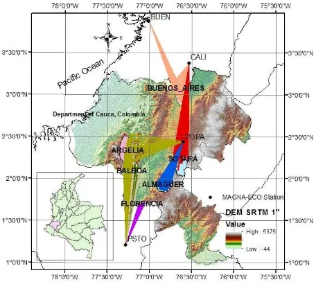
To determine and assess the accuracy of the GPS coordinate measuring instrument for type mapping, the department of Cauca, Colombia was used with the sample coordinates WGS84 77◦22’43,506”W, 1◦36’40,032”N and 76◦31’51,169”W,
3◦08’19,7115”N. This location is characterized by mountainous
areas with steep slopes that hinder wave propagation, affecting accuracy because of the multipath effect and increasing errors in topographic surveys (Ali et al., 2005).
In this study, we analyzed the sources of traceable error by dif-ferentiation, the test method and the results of positioning accu-racy by using static and cinematic GPS relative positioning tech-niques. We considered the following sources of variation post-process: (1) positioning time (2) distance to the base station (2) dilution of precision (3) DEM elevation point, (4) and the GPS mapping equipment model used.
The horizontal errors were analyzed in terms of precision and accuracy. Accuracy refers to the closeness of the sample mean to the true value, and precision is related to the proximity of repeated observations of the mean of a sample (Yoshimura & Hasegawa, 2003).
The precision were evaluated with statistical analysis of database obtained from qualitys parameter of DGPS procedures with soft-ware of both devices.
Further analysis obtained by applying the nonparametric tech-nique of Principal Component Analysis showed relationships be-tween the quality variables reported by the post-process method of differential correction.
2.2 Georeferencing
The method of data collection was carried out with quick local-ization of the attributes on the geometry of the tertiary road net-work, with the use of GPS (Hasegawa & Yoshimura, 2007). The occupancy gaps were 5 minutes for the landmarks, shape 1 in the database of the inventory road, and 1 second for the road axes or shape 2 in the database of the inventory road, using Magel-lan Mobile Mapper 6 receiver, 2009 model and Mobile Mapper 4.6 receiver, 2015 model. The observable ones from the perma-nent stations of the MAGNA-ECO Network of the IGAC at the zero order, Cali and Popay´an, were downloaded, with rates of 30 seconds.
When taking the field points, we used the relative GPS posi-tioning technique, which determines relative positions using one single-frequency receiver and the information of the closest base to establish the vector between two extreme points of a baseline. Since absolute positioning only uses one recipient, the accuracy is low, but in relative positioning, if the distance between the two receivers is not very large, the relative error is good and most errors, such as clock error, orbital error, and atmospheric errors, among others, can be eliminated through differential correction (Dong-feng et al., 2009).
This technique allowed us to take point-type objects or Land-marks with five minutes of positioning in a static mode. However, to achieve adequate precisions, an optimal satellite configuration and favorable weather conditions must exist. In the case of the road axes or polyline-type objects, we used a pseudo-kinematic method wherein the rover goes to each point of the unknown po-sitions in a continuous manner. The time lapse between the first session in one station and the next session should not exceed one hour. This causes an increase in the geometric force of the ob-servations due to changes in the geometry of the satellites that occur during the time periods; that is, with the pseudo-kinematic method, these changes in the satellite geometry are accounted for, so the coordinate information is the best.
The preparation of GPS surveys requires taking into account the Dilution of Precision (DOP), a-dimensional number that reckons the purely geometrical contribution of the satellite position to the uncertainty in a fixed position. The smaller the value is, the better the geometry (Langley, 1999).
The accuracy of the coordinates is determined by post-processing the data; for which downloading data from CORS is required (Continuously Operating Reference Stations) in a RINEX format, uploading the data to computer software (Berber et al., 2012) to possess the raw data recorded in the field.
2.3 Post-processing
A common method for removing the main sources of error and improving the accuracy of positioning is to use the principle of differentiation. With Differential GPS (D-GPS), a mobile unit receives corrections for pseudo-ranges measured from a base sta-tion and obtains the posista-tioning point with the corrected values.
The use of corrected pseudo-ranges improves the accuracy of po-sitioning with respect to the base station.
However, all D-GPS systems suffer from some drawbacks: the requirement for the existence of a base or a reference station; the need for simultaneous observations in both the reference and the unknown point; and the need for a receiver to operate in the neighborhood of the reference station. Since the correlation error decreases with distance, the corrections in the reference station do not replicate the conditions at the rover position. The accuracy of the D-GPS method, in forested areas with single frequency equipment, is considered to be between 2 and 3 m according to studies reported by (Beryouni et al., 2012).
The dispersion of the observations is the standard deviation, for which, the accuracy of each survey is reported as the standard deviation in its horizontal component. With n being the number of times registered, the proprietary software calculates precision as:
The high values of absolute error can show low precision values, suggesting that the analysis of the horizontal absolute error is a better descriptor of performance of the GPS system than the accu-racy calculated by proprietary software (Valbuena, 2010). Some authors agree that the use of the measurement of standard devi-ation is insufficient for the evaludevi-ation of the precision (Sigrist et al., 1999).
The results are expressed in terms of RMS (Root Mean Square) according to the expression:
Where e is the error and n the number of points.
The specifications of precision are based on the assumption that errors follow a Gaussian distribution. The derivation of precision measurements should consider the fact that extreme values exists and that the distribution of errors can be abnormal. Therefore, it is necessary that the precision measurements not be influenced by a skewed distribution of errors. The approach with robust statisti-cal methods allows for the technistatisti-cal treatment of extreme values and separates them from the precision measurements of the fun-damental assumption of a normal distribution (H¨ohle & Ho¨hle, 2009).
If the distribution of errors had a normal behavior and there were no extreme values, the error metrics of the root mean square, the average error and the standard deviation would be appropriate as descriptors of precision, and ranges from the systematic error or mean and standard deviation. If the metric of precision is based on a confidence level of 95%, this range is given by (Mikhail & Ackerman, 1976).
Interval=µ±1.96σ (3)
A robust measure of quality is the median (me), which is a
the precision measurement is obtained by reporting the sampling quantiles of the absolute differences distribution. Absolute errors are used because of the interest in the magnitude of the errors. In addition, absolute errors allow statements of probability with-out having to assume symmetrical distribution. If the problem involve large tails in the error distribution due to a large number of extreme values, an alternative approach to estimate the scale of the errors is the use of a robust scale estimator, such as the Deviation Absolute of the Normalized Median (NMAD) (H¨ohle & H¨ohle, 2009).
N M AD= 1.4826M edianj(|ej−me|) (4)
Where: ej, indicates the individual errors, j, and me is the median of the errors.
3. RESULTS
The results of the GPS precision for the point-type and polyline type objects, obtained in the processes of differential correction of the raw data from the geo-referenced tertiary road network are presented below, under the following parameters: Distance to the base, GPS Horizontal Accuracy -HRMS-, then, a specific analy-sis of the spatial variability for Landmarks and ANOVA test.
3.1 Distance to the base
Figure 1 indicates the position of the differential correction vec-tors of the baseline in the six analyzed municipalities: Almaguer, Argelia, Balboa, Buenos Aires, Florencia and Sotar´a.
Figure 1: Differential correction vectors
The Continuously Operating Reference Stations (CORS) of the SIRGAS network were BUEN, CALI, POPA and PSTO. The baseline vectors had lengths between 3.9 km and 148.5 km (Table 1).
Some researches (Dogan, 2014) have analyzed GPS data with baselines of different lengths, ranging from 6 to 237 km, but with positioning time between 4 h and 24 h. Although the scope of this research was metric precision, the range of the baselines was the same.
Distance to the base (km)
SHP01 SHP02
Municipality Min Max Min Max
Almaguer 57.5 72.3 57.5 72.3
Argelia 66.4 148.5 66.4 148.5
Balboa 87.0 105.1 87.0 109.4
BuenosAires 32.5 118.0 32.5 118.0 Florencia 53.4 63.2 53.4 63.2
Sotara 3.9 133.4 3.45 133.6
Table 1: Distance to the base station in the differential correction process
3.2 Evaluation of precision in the static mode
3.2.1 Precision and accuracy on the geodetic network: For the equipment, we carried out internal and external validity tests of the landmarks of the geodetic network (CC-T-7, GPS-CC-T-8, GPS-CC-T-9, GPS-CC-T-10, 133A-SW-5) from the city of Popay´an, with pre-processing of the Cartesian Plain coordi-nates and calculation of velocity or retiming to 1995. The record-ing periods were 5 minutes. The results of the precision and ac-curacy obtained with the equipment and their corresponding soft-ware are shown in Table 2.
PRECISION ACCURACY
Equipment/Software MM6 MM46 MM6 MM46
MobileMapper6 1,260 1,546 2,523 2,634 MobileMapper46 0,859 1,769 1,657 2,758
RMSE (m) 1,358 2,393
Table 2: Precision and accuracy of equipment
For the test conditions, an average precision of 1,358 m and an average accuracy of 2,393 m were found in terms of Root Mean Square Error. As observed, the error was more critical when found by comparing a pattern than when obtained by the differ-ential correction process or precision, which is consistent with the results of (Yoshimura & Hasegawa, 2003). No significant differences were found in the sensitization of the equipment, the software processing precision (p = 0.02), nor in the accuracy (p = 0.47).
3.2.2 Principal Components Analysis: The decomposition of the main components into a database with geo-referenced land-marks quality information allowed for the establishment of the associations reported in Table 3.
Municipality Correlation Coefficient (r) of HRSM with:
VRSM DIST-BASE DOP
Almaguer 0.93 0.25 0.10
Argelia 0.88 0.16 0.73
Balboa 0.78 -0.17 0.05
BuenosAires 0.89 0.51 0.41
Florencia 0.78 0.20 0.02
Sotara 0.89 0.28 0.34
Table 3: Linear relations between the average horizontal error of Landmarks and the remaining quality parameters
The results seen before indicating the proximity to the base sta-tion did not imply high accuracy. There were other factors, such as the multi-path effect, that affected the precision of the geo-references made. Only one municipality showed a defined linear relationship between the horizontal precision and the precision dilution.
relationship of the horizontal error with the dilution of precision and a low direct linear relationship with the distance to the base or Length variable.
Figure 2: Projection of the quality variables of shape 1 in the first factorial plane
3.2.3 Horizontal error in static mode for landmarks: Table 4 presents the results of the Horizontal Root Mean Square Error parameter, obtained from the processes of differential correction.
Municipality Statistician related with HRSME (m) Min Max Mean Percentile95
Almaguer 0.30 1.86 0.62 1.24
Argelia 0.53 11.65 1.19 1.87
Balboa 0.70 2.83 1.18 2.08
BuenosAires 0.33 3.83 0.79 1.62
Florencia 0.35 1.52 0.90 1.36
Sotara 0.29 4.65 0.98 2.45
Table 4: Horizontal Root Mean Square Error parameter
With the exception of the municipality Argelia 100% of the land-marks placed in the field satisfied the maximum tolerance of 5 m established in the Municipal Road Plans of the Ministry of Trans-port of Colombia. In the municipality of Argelia, although there were only two values greater than 5.0 m accuracy, 99.3% of them were smaller than 5.0 m accuracy.
In the static mode, with positioning times of 5 minutes, we ob-tained horizontal accuracies lower than 2.45 m, corresponding to 95% of the values of the overall horizontal error distribution in the six locations that were analyzed. This results are according to (Beryouni et al., 2012).
3.3 Evaluation of quality in the dynamic mode
3.3.1 Horizontal error in dynamic mode for road axes: For the road axes, in the dynamic mode, the repeatability requirement was not met because each points holding time was only one sec-ond. For these objects, obtained in the dynamic mode, one must take into account the bias or asymmetry of the data and apply robust estimators to consider that effect.
The distribution of errors can be displayed as a histogram of sam-pling errors, where the number of errors or frequency within cer-tain predefined intervals are represented. Such a histogram gives
a first impression of the normal distribution of errors, which can be compared with a normal distribution curve obtained by an or-dinary estimation of the mean and variance error. Due to the presence of extreme values, an estimated curve does not match the data distribution. The reasons why errors do not form a nor-mal distribution are: existence of skewed distributions, which are not symmetrical around the median, or because the distribution is more peaked around the median than the normal distribution while having elongated tails; this latter effect is measured by the kurtosis of the distribution, as shown in Table 5.
Test Alm Arg Bal BnsAir Flor Sot
Skewness 1.4 11.9 12.7 1.7 1.3 1.9
Kurtosis 6.8 207.3 232.7 7.1 5.3 8.3
Table 5: Coefficient of skewness and kurtosis of the HRMS vari-able shape 2
The third order moments indicated a positive asymmetric behav-ior of the distribution of the residual horizontal precision. The municipalities with the more extreme skewed behaviors were Argelia and Balboa.
Another graphic diagnosis tool to check the deviation from the normal distribution is the quantile - quantile (Q-Q) graph Fig-ure 3. The quantiles of the empirical distribution function are drawn against the theoretical quantiles of the normal distribution. If the error distribution is normal, the Q-Q graph should produce a straight line. A deviation from the straight line indicates that the error distribution is not standard. One can also apply formal statistical tests to investigate whether the data originated from a standard distribution, but these tests are often more sensitive to extreme data sets (Ho¨hle & Ho¨hle, 2009). Here, we present the results.
Figure 3: Results of the Q-Q graph as visualization tool of the normality of the GPS horizontal precision
It can be observed that the distribution of the global residuals does not follow a Gaussian behavior and, therefore, robust methods must be applied to treat skewed distributions and report precision metrics.
Metric Alm Arg Bal BnsAir Flor Sot µ(m) 1.52 4.71 3.93 1.50 3.70 2.67
RMSE (m) 1.65 6.19 5.63 1.60 4.32 3.05
σ(m) 0.64 4.02 4.03 0.57 2.23 1.47
Me (m) 1.40 4.25 3.29 1.36 3.51 2.36
MAD (m) 0.37 1.08 0.81 0.30 1.45 0.71
NMAD (m) 0.55 1.59 1.19 0.44 2.14 1.05
Q(68.3) (m) 1.71 5.02 3.94 1.62 4.23 2.89 Q(95) (m) 2.67 8.53 7.34 2.63 8.41 5.53
Table 6: Metrics of precision for the asymmetrical precision of road axes
As can be noted when comparing the results of the 68.3 quantile with the absolute deviation from the standard median, there was a high discrepancy. This reinforces the fact, more so than the nor-mality tests indicated above, that the distribution of the horizontal precision of road axes was not Gaussian and, therefore, the error metric of the Root Mean Square was not appropriate for reporting the precision since it is based on the assumption of normality.
Consequently, the most appropriate metric of precision for skewed distributions was the Deviation Absolute of the Normalized Median; the unscrewed estimator of Standard Deviation in the case of precise symmetric distributions. Since the Deviation Absolute of the Normalized Median is the statistical parameter of precision, we reported that it was affected by a factor of 1.96, which corresponds to a confidence level of 95% as a Probable Circular Error value for purposes of comparison with the reported Tolerance of 5 m defined in the specifications mapping.
Below, we present the results in Table 7 with comparison to the estimated and accepted tolerances. This from the Colombian con-trol agencies for the metric on national road inventories.
Municipality NMAD(m) ECP MaxErr(m) Fit
Almaguer 0.55 1.08 5 Yes
Argelia 1.59 3.12 5 Yes
Balboa 1.19 2.34 5 Yes
BuenosAires 0.44 0.86 5 Yes
Florencia 2.14 4.20 5 Yes
Sotara 1.05 2.05 5 Yes
Table 7: Report of the probable circular error (ECP) and the com-parison with tolerance
In the kinematic mode, we included, with a previous demon-stration of bias in the distribution of horizontal error, the robust estimator of the absolute deviation of the standardized median (Ho¨hle & Ho¨hle, 2009) with a maximum error of 4.20 m, at a confidence level of 95%. These results agree with horizontal po-sitional errors of precision obtained by (Yoshimura & Hasegawa, 2003).
The error corresponds to a scale of 1: 20000, taking in account the maximum error found for a confidence level of 95% (4.2 m) and according to the ASPRS (1990) (Fgdc, 1998) standard.
3.3.2 Multivariate Analysis of quality parameters: An anal-ysis of the principal components among the variables of quality for polyline-type objects, obtained from the differential correc-tion procedure, yielded the following results, Table 8.
Two municipalities had a regular positive linear correlation of horizontal error and dilution of precision. But, this direct rela-tion was low with the elevarela-tion of the points that formed the road axes.
Municipality Correlation Coefficient (r) of HRSM with: VRSM DIST-BASE DOP Elevation
Almaguer 0.84 -0.32 0.09 0.20
Argelia 0.94 0.15 0.65 0.05
Balboa 0.94 -0.05 0.53 -0.10
BuenosAires 0.82 0.34 0.35 0.11
Florencia 0.92 -0.004 0.03 -0.10
Sotara 0.85 0.24 0.26 0.11
Table 8: Linear relations between the average horizontal error of road axes and the other quality parameter
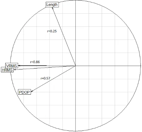
The projection of the variables encased in all the areas of study, of road axes, in the circle of correlations between the PCA, are shown in the Figure 4. We found a strong direct linear relation-ship between the horizontal error and the vertical error, a regular direct linear relationship with the dilution of precision and a low direct linear relationship with the distance to the base and eleva-tion (height).
Figure 4: Projection of the quality variables of shape 2 in the first factorial plane
3.4 Analysis of the spatial dependency
The spatial autocorrelation measures the relationship between the values of the variable according to the spatial arrangement of the values (Cliff & Ord, 1973). A popular measure of the spatial autocorrelation is the Moran Index. The result is positive when nearby areas have a similar value and negative when they have different values close to zero and when the attribute values are randomly organized. The calculation of the index in the munic-ipalities listed in the tables above yielded values of 0.05; 0.02; 1.09; -0.01; -0.02; 0.12. We obtained high spatial proximity to the horizontal GPS error in the municipality of Balboa. However, the only way to obtain an adjustment of a mathematical model of autocorrelation (Webster & Oliver, 2001) to the empirical var-iogram, was the analysis of the total dataset of errors in the six municipalities (Table 9).
Model Null Sill Range MaxDistance
Exponential 0.13 0.64 3741.96 11537.7
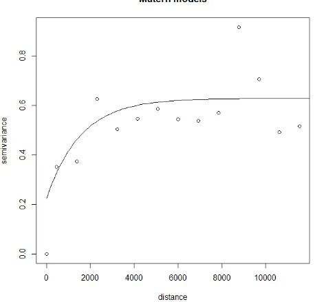
Matern 0.13 0.46 1559.15 11537.7
To predict the horizontal GPS error at the centroids of the six analyzed municipalities, we used the Ordinary Kriging method (Isaaks et al., 1989). This gave an estimate of error for an HRMS prediction (with Matern models) at a confidence level of 95% in the range of 1,968 m to 2,568 m, with an average of 2,347 m (Table 10).
Pt East North HRMS Var Err95%
1 1026945.9 703513.2 0.775 0.603 2.297 2 999527.5 679441.6 0.909 0.467 2.249 3 1044334.5 828103.6 0.632 0.430 1.916 4 980296.8 748882.1 1.024 0.560 2.491 5 985405.9 722313.8 1.093 0.567 2.568 6 1051794.6 738417.9 1.070 0.580 2.563
Table 10: Kriging Ordinary Prediction in the municipality cen-troids
The evaluation of the estimated accuracy of the horizontal error by means of cross validation showed some diagnostic statistics: root mean square -RMS- of 0.20 m and Standardized RMS of 0.23. The latter result, much lower than 1, indicated an overes-timation of the variability of predictions, as can be seen in the setting of the prediction model, Figure 5.
Figure 5: Model of adjusted Matern semivariogram
3.5 External factors that compromise the positional error
ANOVA was used to determine the effect of the equipment model, and the static-cinematic measurement methods for the horizontal GPS error.
According to Table 11, the horizontal precision with the equip-ment used and the two geo-referencing field procedures differed significantly(p < 0.001). But, in the case of the kinematics-method, this results did not occur due to the strong asymmetry of the GPS data.
We found significant differences in the evaluation of the horizon-tal precision with the equipment used and the method of geo-referencing according to (Valbuena et al., 2010).
4. CONCLUSIONS
The internal and external validity tests performed on the equip-ment used in the geodetic network of the city of Popayan, done
Source of variation MeanSq Fstat p-value Static vs Devices 15.87 34.96 <0.001 Method vs DeviceMM6 423.45 280.73 <0.001 Method vs DeviceMM46 3321.23 223.52 <0.001
Table 11: ANOVA results for horizontal precision according to the equipment and method employed
by comparing coordinates at the ITRF1995.4 time, revealed that they complied with the maximum horizontal error tolerance of less than 5 m. However, the external validity or accuracy was higher than the internal validity (precision) indicating that it was more critical in assessing the quality of the GPS geo-references.
The horizontal precision of the static geo-references derived from the differential correction software, in the selected equipment for satellite measurements (300 measurements per point) provided maximum values of 4.65 m. This indicates that the maximum tolerance (<5 m) in 100% of cases was achieved.
As an estimate of the GPS horizontal precision, we selected the robust statistical: Absolute Median Standard Deviation (NMAD) to consider the effect of bias in the residuals without removing extreme values. The NMAD value, affected by a factor of 1.96 for a reliability of 95%, corresponded to maximum value of 4.20 m. The standard errors at two sigma (95% confidence) were less than the specified tolerance of 5 m. As a result, the satellite surveys of the road axes complied with the maximum tolerance of 5 m.
The multivariate analysis of the geo-references quality variables allowed us to conclude that there was a significant direct rela-tionship between the horizontal precision and the dilution of pre-cision in both the static and kinematic modes. On the contrary, the linear relationship decreased with greater distances from the base.
Despite the fact that the results of the horizontal error predic-tion, with the Ordinary Kriging method in the centroids of the analyzed municipalities, showed an overestimation in the predic-tion values, the horizontal GPS error values estimated an average of 2,347 m, similar to the results of the external validation of the equipment (2,393 m). This may indicate the potential of the Kriging method for evaluating the accuracy of geo-references.
The quality evaluation of the geo-references in the static and kine-matic modes showed a horizontal error at a confidence level of 95%, less than 5 m, which corresponds to a scale of 1: 20000. This assessment provides a basis for obtaining a process of at-tributes and validation for current research the semi-automatic detection of landslides at a semi-detailed scale that is being car-ried out in the study area.
REFERENCES
Ali, R., Cross, P., & El-sharkawy, A. (2005). High Accuracy Real-time Dam Monitoring Using Low-cost GPS Equipment High Accuracy Real-time Dam Monitoring Using Low-cost GPS Equip-ment. In FIG Working Week.
Berber, M., Ustun, A., & Yetkin, M. (2012). Comparison of ac-curacy of GPS techniques. Measurement: Journal of the Interna-tional Measurement Confederation, 45(7), 1742 1746. http://doi.org/10.1016/j.measurement.2012.04.010.
Bulletin, 64(11), 2507 2518. http://doi.org/10.1016/j.marpolbul.2012.05.015.
Cliff, Andrew David & Ord, J. K. (1973). Spatial autocorrelation. Pion London, 5.
Dogan, U., Uludag, M., & Demir, D. O. (2014). Investigation of GPS positioning accuracy during the seasonal variation.
Mea-surement, 53, 91 100.
http://doi.org/10.1016/j.measurement.2014.03.034.
Dong-feng, R., Yun-peng, L., & Zhen-li, M. (2009). Test and analysis on the errors of GPS observation in mining field. In Pro-cedia Earth and Planetary Science, 1(1), 1233 1236). http://doi.org/10.1016/j.proeps.2009.09.189.
Fgdc. (1998). Geospatial Positioning Accuracy Standards Part 3: National Standard for Spatial Data Accuracy. World, 28. http://www.fgdc.gov/standards/projects/FGDC-standards-projects/ accuracy/part3/chapter3.
Fiorucci, F., Cardinali, M., Carl, R., Rossi, M., Mondini, A. C., Santurri, L., Guzzetti, F. (2011). Seasonal landslide mapping and estimation of landslide mobilization rates using aerial and satellite images. Geomorphology, 129(1-2), 59 70.
Hasegawa, H., & Yoshimura, T. (2007). Estimation of GPS po-sitional accuracy under different forest conditions using signal interruption probability. Journal of Forest Research, 12(1), 1 7. http://doi.org/10.1007/s10310-006-0245-4.
H¨ohle, J., & Ho¨hle, M. (2009). Accuracy assessment of digital elevation models by means of robust statistical methods. ISPRS Journal of Photogrammetry and Remote Sensing, 64(4), 398 406. http://doi.org/10.1016/j.isprsjprs.2009.02.003.
Isaaks, E. H. S., Isaaks, M. R. E. H., & Srivastava, M. R. (1989). Applied geostatistics. No. 551.72 ISA.
Langley, R. B. (1999). Dilution of Precision. GPS World, 10(May), 5259. http://www.ceri.memphis.edu/people/rsmalley/ESCI7355/ gpsworld may99.pdf.
Malamud, B. D., Turcotte, D. L., Guzzetti, F., & Reichenbach, P. (2004). Landslide inventories and their statistical properties. Earth Surface Processes and Landforms, 29(6), 687 711. http://doi.org/10.1002/esp.1064.
Martin, A. a., Holden, N. M., Owende, P. M., & Ward, S. M. (2001). The Effects of Peripheral Canopy on DGPS Performance on Forest Roads. International Journal of Forest Engineering, 12(1), 71 79.
Mikhail, E. M., & Ackermann, F. E. (1976). Observations and least squares, IEP New York.
Sigrist, P., Coppin, P., & Hermy, M. (1999). Impact of forest canopy on quality and accuracy of GPS measurements. Interna-tional Journal of Remote Sensing, 20(18), 3595 3610
Valbuena, R., Mauro, F., Rodriguez-Solano, R., & Manzanera, J. a. (2010). Accuracy and precision of GPS receivers under forest canopies in a mountainous environment. Spanish Journal of Agricultural Research, 8(4), 1047 1057.
Webster, Richard & Oliver, M. A. (2001). Geostatistics for envi-ronmental scientists (Statistics in Practice). Wiley
Yoshimura, T., & Hasegawa, H. (2003). Comparing the precision and accuracy of GPS positioning in forested areas. Journal of
For-est Research, 8(3), 147 152.
http://doi.org/10.1007/s10310-002-0020-0
ACKNOWLEDGEMENTS