AN EFFICIENT METHOD TO CREATE DIGITAL TERRAIN MODELS FROM POINT
CLOUDS COLLECTED BY MOBILE LiDAR SYSTEMS
L. Gézeroa,b, C. Antunesc
a Faculdade de Ciências, Universidade de Lisboa, 1749-016 Lisboa Portugal
b LandCOBA, Consultores de Sistemas de Informação e Cartografia Digital Lda - [email protected] c Instituto Dom Luiz, Faculdade de Ciências, Universidade de Lisboa, 1749-016 Lisboa, Portugal - [email protected]
KEY WORDS: Mobile systems, point cloud, Digital Terrain Models, LiDAR, Delaunay triangulation, Laplacian operator
ABSTRACT:
The digital terrain models (DTM) assume an essential role in all types of road maintenance, water supply and sanitation projects. The demand of such information is more significant in developing countries, where the lack of infrastructures is higher. In recent years, the use of Mobile LiDAR Systems (MLS) proved to be a very efficient technique in the acquisition of precise and dense point clouds. These point clouds can be a solution to obtain the data for the production of DTM in remote areas, due mainly to the safety, precision, speed of acquisition and the detail of the information gathered. However, the point clouds filtering and algorithms to separate “terrain points” from “no terrain points”, quickly and consistently, remain a challenge that has caught the interest of researchers. This work presents a method to create the DTM from point clouds collected by MLS. The method is based in two interactive steps. The first step of the process allows reducing the cloud point to a set of points that represent the terrain’s shape, being the distance between points inversely proportional to the terrain variation. The second step is based on the Delaunay triangulation of the points resulting from the first step. The achieved results encourage a wider use of this technology as a solution for large scale DTM production in remote areas.
1. INTRODUCTION
LiDAR is a non-selective technique, i.e., the georeferenced point clouds represent the surrounding physical reality at an acquisition moment, indiscriminately, with no classification and including: terrain, vegetation, buildings, or any other object within the system range. So, for using that kind of data for DTM generation, it is necessary to identify and to classify the points from the cloud that represent the shape of the terrain.
This subject has challenged many researchers since the first LiDAR systems appeared. Many techniques and approaches, being more or less effective, were developed in the recent years. Chen et al. (2017) provide a good review of the state of the art methods for the generation of MDT techniques using point clouds generated by Aerial LiDAR Systems (ALS). Despite the extensive review and great progress that has been made, it is recognized by these authors that the generation of DTM remains a challenge, in certain situations.
The majority of the published work (for e.g., Özcan and Ünsalan, 2017) in this field of study is based in point clouds from collected from ALS. One reason for that may be the fact that MLS technology is more recent. However, the point clouds collected by MLS present very different characteristics from those collected by ALS. The different collection angle, the high density of information and the complexity of the environment surrounding the road, cause that most of the techniques for DTM creation from ALS data do not work or are not very efficient in data collected by MLS.
Nevertheless, there are some studies that adapt filters initially designed for ALS, or apply specific algorithms for MLS (Fellendorf, 2013; Pfeifer and Mandlburger, 2008; Tyagur and Hollaus, 2016; Vallet and Papelard, 2015; Yen et al., 2010). This work intends to contribute in this research topic, by proposing a novel method based on two main steps that comprise an iterative grid division and the establishment of neighborhoods by using an adapted version of the Laplacian operator.
Obtaining the DTM from the road and surrounding area, with sufficient detail and precision, is a need for design projects to establish water and sanitation networks, asphalt laying and road improvement. This need is even more significant in developing countries. However, the collection of the data to generate the DTM is more difficult in those areas, either due to the lack of skilled workforce, security issues, or due to the fact that these projects are located in remote areas where production costs are not compatible with the available resources. The MLS allow fast collection of large amounts of data along the roads, reducing the fieldwork time, when compared with classic topographic methods, which has implications on lowering acquisition costs and increasing safety.
The implementation of the proposed method arose from the need for an efficient method to generate the DTM from MLS point clouds, allowing to take advantage from the MLS efficiency. The goal is to maintain the precision of the data gathered and at the same time not to be a bottleneck in the information process workflow.
A challenge for the DTM generation methods is the adaptation capacity to various environments (rural and urban), where the features and terrain shapes that surround the roads are very different. It is also noteworthy the amount of points in the final DTM, since the large number of points in the cloud and in the DTM generated from them are usually pointed out by users as a limitation to wider use. The points included in the DTM must be the minimum as possible but, at the same time, must be enough to ensure the representation of the terrain shape at a certain scale. The remaining of the paper is composed as follows. In section 2 the description of the two steps of the method is carried out, as well as the description of the method’s parameters. A sensitivity analysis of the method’s parameters, and the results obtained in different environments and in the most sensitive terrain shapes for DTM generation are presented in section 3. It also includes a summarized application of the proposed method in two point clouds collected in Angola and Brazil. Finally, conclusions and future work are provided in section 4.
2. METHOD DESCRIPTION
The proposed method consists of two main, iterative and complementary steps.
Step 1: The purpose of the first step is to decrease the number of the cloud points used in the DTM, to accelerate the subsequent processes, while keeping a point distribution so to have a good representation of the terrain shape.
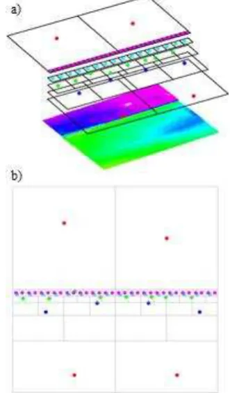
The grey points in Figure 1 portray a point cloud collected by an MLS, where each point is represented by its tridimensional coordinates (X, Y, Z). Initially, a regular grid is established along the entire area covered by the point cloud. Inside each grid cell the point from the cloud (PZmin) that has the smallest Z coordinate value (red points in Figure 1) is identified. Then each of these initial cells is divided into four new equal size cells. To choose the point that represent each of the new cells, an elevation restriction is applied. That restriction is based in the Z value of the PZmin point of the cell, which gave rise to it. An interval is established that is limited by a minimum Z value (LMin) and a maximum Z value (LMax). So, for each new cell, the candidates cloud points (PC) are selected based in the condition PZmin(Z) + LMin < PC(Z) < PZmin(Z) + LMax. Among the candidate’s points that meet this restriction, the point with the lowest Z value is chosen (blue points in Figure 1). This process is repeated iteratively until a stopping criteria is reached. The stopping criteria can be established by the number of iterations or until a minimum cell dimension is reached. It is possible to establish a relationship between the number of the iterations and the size of the cell in this iteration through Equation 1.
D � = ����
�− 2 (1)
Where i = the iteration number
DIni = the initial cell dimension value D(i) = the side cell size in iteration i
Figure 1. Schematic iterative division of the cells
On one hand, by choosing in each iteration a point inside the resulting cells that is greater than PZmin(Z) + LMin, it allows to guarantee an evolution of the represented terrain in the Z direction. On the other hand, by setting a maximum limit of PZmin(Z) + LMax it ensures that fewer points of cars, trees, houses or other points outside the terrain are considered in the process. The restriction to the points inside the cells at each iteration can be represented by Equation 2.
����= Min Z �� → {ℎ��� ���� + ��+ ����< �> ��
The LMin value is directly related to the detail intended for the final DTM. By using smaller LMin values it produces smaller Z variation between the points in each iteration, so smaller variations of the terrain are represented and consequently the resulting DTM will have more detail. However, low values for LMin lead to a DTM solution with many more points. The value shall be established taking into account the desired scale for the final DTM.
To better exemplify the process, let us consider an initial cell in which all cloud points (PC) in its interior represent an approximately horizontal road. If PZmin is the point with the smallest Z value inside the cell and if none of the points inside the cell satisfies the condition PZmin(Z) + LMin < PC(Z), then no point is associated to the new four cells resulting from the initial cell division. In this case the process stops inside the cell and the DTM is represented by only one point in the inner space of the cell.
The LMax value is established to limit situations where the minimum value within a given cell has a very large difference with respect to the cell point that gave rise to it. For example, if we consider a cell containing points representing a road and branches of a tree over the road, in a first iteration the lowest point inside the cell will have the Z value of the road (PZmin), in the following iteration, the Z value of all the points representing the road will not satisfy the condition PZmin(Z) + LMin < PC(Z). The only points that satisfy this condition are the ones that represent the tree branches. Considering that the defined LMax value is less than the height of the branches in relation to the road, all points of the tree branches do not satisfy the condition PZmin (Z) + LMax> PC(Z) and will not be considered for the DTM. A great advantage of this process is that the resulting points are not equidistant, being the distance between them inversely proportional to the terrain variation.
The Figure 2a) represents a point cloud colorized by height, and the schematic representation of the result of Step 1 over the area.
Figure 2. a) Perspective view of a colored point cloud and cells with the corresponding points inside; b) Top view of the cells and selected points.
The top view of the resulting points is shown in Figure 2b), where the irregular point distance inversely proportional to terrain variation can be observed along the terrain break. The different point colors represent different iterations.
Given the large number of points in the cloud, the difficulty in handling them is often a constraint to the use of the cloud and the resulting DTM. The discretization of the points from the cloud through this method allows to decrease the number of points of the DTM, maintaining, however, those that realistically represent the terrain shape. This process makes an easy handling of the DTM through applications and processors with lower requirements, allowing the use of them by users less familiar with point clouds. Obviously, the terrain within each cell is not necessarily quasi-perpendicular to the Z coordinate axis. In sloping areas, the number of points for the terrain representation will be much higher than the necessary, even if the terrain within a given cell is approximately flat.
At the end of this step, the number of points inside a cell will be at most equal to the number of cells resulting from the initial cell division, which will be much lower than the number of points in the initial cloud. The remaining redundant points will be eliminated in the second step of the method.
A prerequisite to obtain the right result of step 1 is the need that the point with the minimum Z of each of the initial cells be in the ground, because the whole process is triggered within each cell based on this assumption. If that starting point of a given cell is above the ground, (over an object outside the terrain, such as a car, a house or a tree) all points resulting from the process inside that cell will not represent the terrain. On the other hand, although in theory no cloud point is below the ground, points in this situation are quite common. These points usually result from reflections of the LASER pulse on mirrored surfaces, such as windows or water, which leads to the deviation of its path, a delay in the travel time, and consequently to an error in the point position. Both situations are critical for the quality of the final result. Figure 3 portrays the effect of a low outlier in the final DTM. On one hand, if the point cloud only includes points on and above the ground, the increase of the initial cell size also increases the chances of the PZMin to be located on the ground. Small initial cells are more likely to only include points above the ground (for example, a part of a car or a house). On the other hand, as shown in the results, the DTM resolution will be lower, when the initial cell size is larger. Likewise, the removal of outliers below the ground is a complex task.
Figure 3. Erosion process caused by low outlier
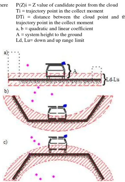
For MLS collected point clouds it is possible to use the information associated to the trajectory in order to restrict the number of candidate points and also to reduce the probability of
the points to be located far away from the terrain. Considering that the MLS trajectory can be represented by a sequence of points over time (Ti), there is a temporal relation between each one of the cloud points and the moment of the trajectory in which this point was obtained.
When reducing the time interval (T) between two trajectory consecutive points to the frequency of the used Inertial Measurement Unit, the cloud points obtained in the interval T create a cross section, so the cloud can be reduced to a set of these cross sections. Since the vehicle carrying the MLS travels along the road, and consequently on the ground, it is possible to use the trajectory to establish a vertical range limited by values Ld and Lu, where the points outside that range are away from the ground (down and up, respectively) and will not be considered in the process. Thus, it is sufficient to apply a quadratic function (Equation 3) to each cross section that allows the generalized adaptation to different types of terrain.
In Figure 4 several terrain situations are presented. Adapting the parameters to the terrain shape will help to get better results from step 1, especially in urban areas where more reflective surfaces exist. In case that several terrain changes occur and it is not possible to define a trend, the range (Ld, Lu) can be increased in a way to include all terrain points but still eliminating the outliers.
{� � − � < ��� + ��� + �� − �
� � + �� > ��� + ��� + �� − � (3)
where P(Z)i = Z value of candidate point from the cloud Ti = trajectory point in the collect moment
DTi = distance between the cloud point and the trajectory point in the collect moment
a, b = quadratic and linear coefficient A = system height to the ground Ld, Lu= down and up range limit
Figure 4. a) Linear restriction with a=0 and b=0 b) Quadratic restriction with a>0 c) Quadratic restriction with a<0
It is important to emphasize that the previous application of this restriction only intends to eliminate outliers significantly away from the ground, to which the process is very sensitive. The points that are closer to the ground will be eliminated in the smoothing process applied in Step 2 of the method.
Step 2: In this step, a Delaunay triangulation is performed, using the points resulting from step 1. The triangulation process becomes much faster due to the discretization of the cloud points made in step 1. In addition, those points ensure the creation of a surface much closer to the reality of the terrain, eliminating incongruent situations, namely when two or more points have the same planimetric (X, Y) coordinates, but different values of Z. The Laplacian operator is perhaps the most known and used smoothing operator (Belkin et al., 2008). This operator is based in the establishment of a neighborhood relation through the triangles with shared edges. Figure 5 presents an example of the establishment of a neighborhood, where the red points represent the neighborhood of the blue point.
Figure 5. Neighborhood relation through the shared edges.
The original version of the Laplacian algorithm is quite simple: the position of the blue point (and the corresponding triangle vertex) is replaced by the average point of the neighbor’s positions (red points) (Vollmer et al., 1999).
In this work, instead of changing the point position, the point is removed from the final DTM. Different operators are suggested based on the defined neighborhood. For example, the TriMin and TriMax values (Figure 5) represent the corresponding minimum and maximum lengths of the edges established for the neighborhood.
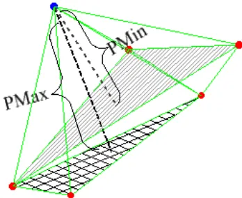
Another operator to be used in this work is based on the plane or planes generated by the neighboring points (Figure 6).
Figure 6. Example of the minimum distance (D) from a point to the plane defined by three neighboring points.
In Figure 6, the distance D represents the minimum distance between the blue point and a plane generated by the tree neighboring points (red points). In order to calculate D it is necessary to determine the plane equation from the three-dimensional coordinates of the points.
Considering the general equation of a plane as ax + by + cz + d = 0, the a, b, c and d coefficients can be obtained from a vector normal to the plane. The normal vector is computed from the cross-product of two vectors connecting the points. Then, the distance D is calculated through Equation 4, where (X0, Y0, Z0) are the blue point coordinates.
� = + + +
√ + + 4
In the case where a point has more than three neighbors, it is likely that not all stand on the same plane. In this case, statistical methods can be applied to obtain the mean plane, namely by least squares or by defining all the planes that are generated by grouping the neighbors three by three and calculating all the minimum distances between the generated planes and the point. In Figure 7, the values PMax and PMin represent the corresponding minimum distances to the furthest and the closest planes generated by the three grouped neighbors.
Figure 7. Minimum and maximum plan distance.
The goal of using these operators is to eliminate all conspicuous points by smoothing the surface generated by the points resulting from step 1, and to eliminate the points in quasi-plane areas, which are not relevant for the representation of the terrain. The step 2 is applied through an iterative process. Two values of distance, D1 and D2 are established. In each iteration a new Delaunay triangulation is created, and the points where D1 > PMax or D2 < PMin are eliminated. D1 and D2 may be adjusted according to the desired result. Taking into account that neighborhood is reciprocal i.e., a certain point belongs to the neighborhood of each of the neighboring points, in order to avoid an erosion of the model, a constraint is applied in each iteration. Based on that constraint, if any neighbor of a point is identified to be eliminated from the model, that point cannot be eliminated in that iteration, regardless of satisfying the condition ‘D1 > PMax or D2< PMin’. The stopping criteria for the iterations can be established by an absolute minimum value for the number of eliminated points or by setting a minimum value for the eliminated points between consecutive iterations.
It should be noted that the resulting points from Step 1 and Step 2 are points directly measured from the clouds, with no interpolation process.
3. RESULTS
In order to test the different steps of the proposed method, C# algorithms were implemented. This section depicts the obtained results by the application of the two steps in point clouds collected by MLS. A sensitivity analysis of the proposed method The International Archives of the Photogrammetry, Remote Sensing and Spatial Information Sciences, Volume XLII-1/W1, 2017
parameters is presented. The following examples data were also chosen to demonstrate the application of the method in rural and urban environments.
3.1 Sensitivity analysis
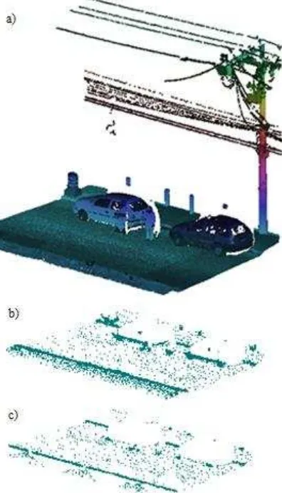
Figure 8a) shows a point cloud sample in a rural area with trees. Figure 8b) presents the result obtained by applying Step 1 to the sample cloud of Figure 8a). It can be verified that the cloud points representing the vegetation, the house wall, electric power lines and poles were globally eliminated, keeping only points at the terrain level. It is also observed that the resulting points do not have a regular density, being the density smaller in plane areas, for example along the road, and higher in areas with greater terrain variation.
Figure 8. a) Point cloud example colored by height b) Resulting points obtained from Step 1 application after four iterations, where DIni = 1 m, LMin = 0.04 m, LMax = 0.08 m.
The results obtained by the variation of the initial cell dimension (DIni) are presented (Figure 9). The remaining parameters values are the same as used in Figure 8b). By decreasing the DIni value, the resulting points’ density increases, allowing a better representation of the terrain details.
Figure 9. a) Point cloud in urban area colored by height b) Step 1 result with DIni = 4 m c) Step 1 result with DIni = 2 m d) Step 1 result with DIni = 1 m.
One of the great challenges in DTM creation and representation is the modelling of the terrain break lines, being the line along the curb in urban areas a good example of this. In Figure 10, a cross section of a point cloud crossing a curb is presented. The cross section has a width of 0.25 m and a length of 2 m. It is also presented with red points the obtained result as the number of iterations of Step 1 increases. In the first iteration (Figure 10a)) it is only observed the points with the lowest Z value (PZMin) inside the initial cells. As the number of iterations increases (Figures 10b) and 10c)), the division of each of the initial cells allows a greater discretization of the terrain and consequently increases the number of points.
Figure 10. a) Step 1 result with one iteration b) Step 1 result with two iterations c) Step 1 result with three iterations.
By increasing the number of iterations, a greater concentration of points takes place in the break line area of the curb, while in the horizontal areas the density does not increase. This effect results from the fact that in the following iterations, in the quasi horizontal areas, none of the points inside the cells satisfy the constraint of Equation 2, and the process is stopped inside these cells. In the areas of greater terrain variation the cells continue to divide until there are no more points that satisfy the condition or until the stop criteria is reached. This explains the fact that the distance between the resulting points is inversely proportional to the variation of the terrain.
Parked cars along roads are another typical issue in DTM creation from point clouds collected in urban environments. Figure 11a) shows a point cloud where two parked cars were captured by the MLS data collection. Figures 11b) and 11c) compare the obtained results of step 1 by variation of LMax value. By decreasing the LMax value (Figure 11c)), the number of points representing the vehicles in the final result also decrease. That happens because the LMax value used in the example shown in Figure 11c) is less The International Archives of the Photogrammetry, Remote Sensing and Spatial Information Sciences, Volume XLII-1/W1, 2017
than the distance between the car floor and the ground. Thus, the step1 applied to the cells containing the points from the car stops before reaching those points. The only points representing the car that remain in the Figure 11c) are the points from the car wheels that are in contact with the ground. In Figure 11b), the points representing the car floor that are collected directly or through the car window remain in the result. The result presented in Figure 11c) turns much easier the elimination of the car points in step 2. In the Figure 11b) result, it will be more difficult to eliminate those car points and at the same time keeping, for example, the points representing the curb.
Figure 11. a) Point cloud sample, colored by elevation b) Step 1 result with LMax = 0.40 m c) Step 1 result with LMax = 0.15 m.
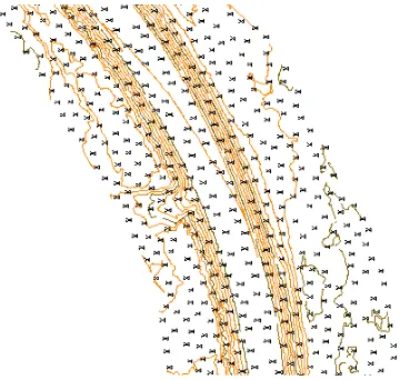
In the application of Step 2, the S-hull algorithm (Sinclair, 2010) was selected to implement the Delaunay triangulation, among the various algorithms described in the literature.
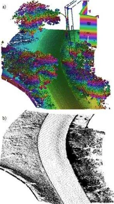
Figure 12a) shows a hill shade representation of the Delaunay triangulation based in the points of Figure 8b).
Although the surface appears to make a correct representation of the terrain, if an amplified zone is observed (Figure 12b)), it can be verified that there are many peaks particularly in the undergrowth areas. This effect will be decreased by the application of step 2.
Threshold values of PMax and PMin are defined. The goal is, on one hand, the elimination of conspicuous points and smoothing the surface and, on the other hand, the decrease of the number of the DTM points, keeping the terrain details, namely, the break lines along the terrain.
Figure 12. a) Hill shade representation of the Delaunay triangulation of Figure 8a) result b) Amplified red area of Figure 12a).
Figure 13 represents the same amplified area of Figure 12b), after the application of step 2. The result was obtained with the restrictions PMax > 0.05 m and Trimax < 0.75 m. That means that in each iteration all points that satisfy both conditions are eliminated. Besides that, in each iteration, no point can be eliminated if any of its neighbors are identified to be eliminated. The number of points have been reduced from approximately 122000 in Step 1 result (Figure 8b)) to 53000 points (a reduction of 57%). The presented result was obtained after 37 iterations and took 42 seconds.
Figure 13. Result obtained after Step 2 application with PMax > 0.05 m and Trimax < 0.75 m.
Together with the smoothing process, the PMin value was used to decrease the number of points in flat areas. Figure 14 shows the difference between the Delaunay triangulation of the Step 1 result (Figure 14 a)) and the Step 2 result using PMin < 0.005 m The International Archives of the Photogrammetry, Remote Sensing and Spatial Information Sciences, Volume XLII-1/W1, 2017
and TriMin < 0.5 m (Figure 14 b)). Despite the fact that a lower point density can be observed in flat areas, the curb line is still well defined.
Figure 14. a) Delaunay triangulation of Step1 result b) Delaunay triangulation of Step1 result and PMin < 0.005 m and TriMin < 0.5 m.
Using the parameters of Figure 13 and Figure 14b) on step 2, it was possible to decrease the number of points to approximately 8000. Starting from the point cloud shown in Figure 8a), with 1238000 points, it took around 70 seconds in total to run both steps 1 and 2. The resulting data set has a decrease of 99% of the initial points that are comprised of non-ground and redundant points. The remaining data set includes points that are part of the terrain and are enough to create a realistic DTM.
3.2 Case studies of Angola and Brazil
The proposed method was applied in two MLS data collections along roads in different areas of the globe, Brazil and Angola. Both are developing countries with huge infrastructures needs and the corresponding need of basic geographic information to support their project design, namely DTM. In the Angola study case, it is intended to obtain a DTM from a rural road in Luanda surroundings. The purpose of the DTM is to be used as a basis to the project design of a road asphalting. The data from Brazil was collected in an urban neighborhood of Rio de Janeiro, and its purpose is the project design of a sanitation network.
The collected point clouds were obtained by different systems and processed by different software applications. In both cases the clouds were exported to LAS 1.2 file format (Specifications in Table 1).
Country MLS LAS number Lenght
Angola Trimble MX8 8 12 Km
Brazil Optech Lynx 19 23 Km
Table 1. Main data collection specifications
The LAS number in Table 1 corresponds to the number of the standard LAS files obtained in each data collection. The files can be split by the operator in the vehicle at the collection moment or in the cloud processing software.
First, the step 1 and step 2 were applied in sequence to each LAS file independently. For each LAS file an ASCII file was created with the resulting points. That allows to reduce the number of points in a way to subsequently merge the ASCII files. Step 2 is again applied to the merged ASCII file to get the DTM points for the entire collected area.
Figure 15. Overall view of the Brazil DTM final result.
The final DTM comprise approximately 248000 points in Brazil (Figure 15) and 65000 in Angola.
Figure 16 shows a sample area of the Angola final result. The DTM is represented by contours with 0.5 m distance and elevation points. The presented elevation points were chosen directly from the resulting DTM points with no interpolation.
Figure 16. Angola data set area.
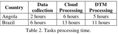
Table 2 describes the processing time for each task of the process. The International Archives of the Photogrammetry, Remote Sensing and Spatial Information Sciences, Volume XLII-1/W1, 2017
Country Data collection
Cloud Processing
DTM Processing Angola 2 hours 6 hours 5 hours Brazil 6 hours 13 hours 11 hours
Table 2. Tasks processing time.
The planning time, travel, GPS reference establishment, control points measure and data transfer are not included in Table 2, but even so it can be used to compare the different tasks processing time and to show that the proposed method can be applied without having the processing time as a bottleneck of the entire process.
4. CONCLUSIONS AND FUTURE WORK
This work proposes a novel method to create DTM from MLS collected point clouds. Besides the process description, a sensitivity analysis is presented to demonstrate the adaptation capacity of the model to different environments. The method behavior in the most typical issues in DTM creation, like break lines, is also presented.
The resulting DTM points are not equidistant, which allows the creation of a more detailed model with less points. The remaining points belong to the initial points cloud, with no interpolation. Since the method is very sensitive to outliers, a procedure to eliminate the points most apart from the terrain is depicted. There are still some ongoing work, especially to create the DTM in heterogeneous areas included in the same point cloud. Perhaps a pre-process can be included in the method to determine the best parameters to different terrain environments, which is recommended as future work.
Despite that, the simplicity of the method and the results obtained by its application in data collected from different systems and in different countries, are encouraging and they justify the pursuing for methods improvement.
REFERENCES
Belkin M., Sun J., Wang Y., 2008. Discrete Laplace operator on meshed surfaces. In Proceedings of SOCG 2008, pp. 278–287.
Chen, Z., Gao, B., Devereux, B., 2017. State-of-the-Art: DTM Generation Using Airborne LIDAR Data, Sensors, 17(1): 150. doi: 10.3390/s17010150.
Fellendorf, M., 2013. Digital terrain models for road design and traffic simulation. In: Photogrammetric Week '13, 309-317. Stuttgart, Germany.
Özcan, A. H., Ünsalan. C., 2017. LiDAR Data Filtering and DTM Generation Using Empirical Mode Decomposition. In: IEEE Journal of Selected Topics in Applied Earth Observations and
Remote Sensing, Vol. 10(1): 360-371. doi:
10.1109/JSTARS.2016.2543464.
Pfeifer, N., Mandlburger, G., 2008. Lidar data filtering and DTM generation, In: Shan, J., Toth, C. K. (eds.). Topographic Laser Scanning and Imaging: Principles and Processing, CSC Press, pp. 308-333.
Sinclair D. A., 2010. S-hull: a fast sweep-hull routine for Delaunay triangulation. Http://www.s-hull.org (29 March 2017).
Tyagur, N., Hollaus, M., 2016. Digital Terrain Models From Mobile Laser Scanning Data. In: The International Archives of Photogrammetry, Remote Sensing and Spatial Information Sciences, Prague, Czech Republic, Vol. XLI, Part B3, pp. 387-394.
Vallet, B., Papelard, J. P., 2015. Road orthophoto/DTM generation from mobile laser scanning. In: ISPRS Annals of Photogrammetry Remote Sensing and Spatial Information Sciences, La Grande Motte, France, Vol. 3, Part W5, pp. 377-384.
Vollmer, J., Mencl, R., Muller, H., 1999. Improved Laplacian Smoothing of Noisy Surface Meshes. In: Brunet, P., Scopigno, R., Eurographics, Vol. 18 (3).
Yen, K. S., Akin, K., Lofton, A., Ravani, B., Lasky, T. A., 2010. Using mobile laser scanning to produce digital terrain models of pavement surfaces. Davis, CA: AHMCT Research Center. The International Archives of the Photogrammetry, Remote Sensing and Spatial Information Sciences, Volume XLII-1/W1, 2017