On the moments of ruin and recovery times
q
Alfredo D. Eg´ıdio dos Reis
∗,1Departamento de Matemática, ISEG, Universidade Técnica de Lisboa, Rua do Quelhas 6, 1200-781 Lisboa, Portugal
Received 1 September 1999; received in revised form 1 April 2000; accepted 30 June 2000
Abstract
In this paper we consider the calculation of moments of the time to ruin and the duration of the first period of negative surplus. We present a recursive method by considering a discrete time compound Poisson process used by Dickson et al. [Astin Bull. 25 (2) (1995) 153]. With this method we will also be able to calculate approximations for the corresponding quantities in the classical model. Furthermore, for the classical compound Poisson model we consider some asymptotic formulae, as initial surplus tends to infinity, for the severity of ruin, which allow us to find explicit formulae for the moments of the time to recovery. © 2000 Elsevier Science B.V. All rights reserved.
JEL classification: G22; C69
Keywords: Time to ruin; Probability of ruin; Duration of negative surplus; Severity of ruin; Discrete time model; Recursive calculation
1. Introduction
In this paper we consider recursive algorithms for the calculation of the moments of the random variables time to ruin and the duration of the first period of negative surplus (or time to recovery). As far as the time to ruin is concerned, much has been said in the actuarial literature about the study of the ruin probabilities, whether finite time or ultimate. The study of some existing moments like the expected value or the variance of the time to ruin can give another insight, although somehow limited. For practical purposes it may be useful for instance to have a quick look at how long it takes for ruin to occur, before going into more details like computing ruin probabilities. The proposed method is easy to implement and its outcome is easily interpreted. About the other random variable, the duration of negative surplus has been previously discussed by Eg´ıdio dos Reis (1993) and Dickson and Eg´ıdio dos Reis (1996). The former reference deals exclusively with the moments of this random variable only concerning the classical model, giving closed formulae which depend on the severity of ruin related quantities. In that paper it is also shown the relation between time to ruin and time to recovery when initial surplus is zero. This is important in our work too by providing a starting point in the proposed recursions, as we will see later in the text.
We use a discrete model as a discrete time compound Poisson process first introduced by Dickson and Waters (1991) and later retrieved by Dickson et al. (1995). Under this model we develop a recursion to compute moments
qPart of this work was carried out during the author’s stay at the Centre for Actuarial Studies at The University of Melbourne. Support from
FCT/PRAXIS and ISEG is gratefully acknowledged. ∗Tel.:+351-2139-25867; fax:+351-2139-22781.
E-mail address: [email protected] (A.D. Eg´ıdio dos Reis). 1http://www.iseg.utl.pt/∼alfredo.
of the above quantities, particularly the first two moments, provided they exist. This proposed discrete model not only has interest on his own but also provides numerical approximations for the corresponding quantities in the classical model. We will focus our attention to the discrete model in a way such that it provides an approximation to the classical continuous model.
As far as the time to ruin in the classical model is concerned, Lin and Willmot (2000) show formulae for the computation of the moments by means of renewal equations, particularly the first two moments. With their method, exact evaluation of the moments is straightforward when the claim size distribution is a combination of exponentials or a mixture of Erlang distributions.
Concerning the duration of negative surplus in the classical model, its moments depend on the same quantities of the severity of ruin as shown by Eg´ıdio dos Reis (1993). When initial surplus is zero the moments have a simple formula. For positive initial surplus (and also when it is zero) again, Lin and Willmot (2000) show expressions for the moments of the severity of ruin which will allow us to compute the moments of the time to recovery. Like in the case for the time to ruin they show that exact evaluations can be done easily for combinations of exponentials and mixture of Erlang claim size distributions. Furthermore, we show in this paper that we can also get a simple expression for the asymptotic moment generating function of the severity of ruin, as the initial surplus goes to infinity, which allows us to compute, at least numerically, moments for the severity of ruin as well as the related random variable time to recovery.
Approximations to the duration of negative surplus quantities in the classical model can be done via the severity of ruin using available methods, like the one presented by Dickson et al. (1995), who use the same discrete time model. The approach we present shows how we can do it dealing in full with the discrete model. Not only does it give exact results as far as the discrete model is concerned but it also provides the starting values (when the initial surplus is zero) for the recursions concerning the time to ruin by enhancing the relationship between time to ruin and time to recovery when the initial surplus is zero.
In the next section we introduce the basic continuous time surplus model as well as the discrete model that approximates the basic model, including definitions and notation. In Section 3 we present recursions for the moments of time to ruin for positive values of the initial surplus considering the discrete model. In Section 4 we consider for the discrete model the recursions for the duration of a first period of negative surplus, showing the relationship between time to recovery and severity of ruin. In Section 5 we discuss the starting values, with initial surplus equal to zero, for the recursions in the two previous sections, based on the fact that the time to ruin and the duration of negative surplus have the same distribution. In Section 6 we show some asymptotic formulae for the severity of ruin and, consequently, for the time to recovery considering the classic model. Finally, in the last section we consider a couple of examples showing the kind of approximations in the classical model we can expect to obtain from the recursions formerly discussed. Namely, an exponential, a combination of two exponentials and an Erlang(2) claim amount distributions.
2. Models and notation
We first introduce the classical compound Poisson model. Let{U (t )}t≥0be a classical continuous time surplus process, so that
U (t )=u+ct−S(t ), t ≥0,
whereuis the insurer’s initial surplus,cthe insurer’s rate of premium income per unit time,S(t ) = PN (t )i=1Xi
the aggregate claim amount up to timet,N (t )the number of claims in the same time interval having a Poisson (λt) distribution, and{Xi}∞i=1a sequence of i.i.d. random variables representing the individual claim amounts. We
denote byP (x)andp(x)the distribution and density function ofXi, respectively, withP (0)=0, so that all claim
Xi bypk. We will further assume in some parts of the paper the existence of the moment generating function ofXi,
which we denote bym(t ), and we state that clearly. We define a positive parameterθto be such that
c=(1+θ )λp1,
so that θ is the insurer’s premium loading factor. Without loss of generality, we will make the following two assumptions:c=p1=1. We will refer to this process as our basic process.
We want to produce a discrete approximation to this basic process and we will consider Dickson et al. (1995) approach considering a discrete time Poisson process
Ud(t )=u+t−Sd(t )
fort =1,2, . . ., with an initial reserveu(u=0,1,2, . . .) andUd(0)=u. Also, we have the following:
• Sd(t )is the aggregate claim amount up to time t, and we denote by F (x, t )andf (x, t )the distribution and density function ofSd(t ).
• Individual claims are i.i.d. random variables on the non-negative integers with meanβ >0. Like in the classical model, we will require the existence of higher moments of individual claims, and we will denote thekth moment about the origin bybk (b1=β).
• Premium income per unit time is 1.
• Expected number of claims per unit time isλd=λ/β.
For simplicity we statefj =fd(j,1)andFj = Fd(j,1)forj = 0,1,2, . . .. Notice that Sd(t )is the sum of
i.i.d. random variables, each with probability function{fj}∞j=0. IfXd,ndenotes the aggregate claim amount from
timen−1 until timen, thenSd(t )=Ptn=1Xd,nandfj is the probability ofXd,ntaking valuej. Values forfj,
j =0,1,2, . . ., can be obtained using Panjer’s (1981) recursion. Time to ruin in the basic process is denoted byT and defined as
T =
(
inf{t :U (t ) <0},
∞ifU (t )≥0 for allt >0,
finite time ruin probability from some initial surplusu≥0 is defined as
ψ(u, t )=Pr[T ≤t|U (0)=u],
and ultimate ruin probability ψ(u) = Pr[T < ∞|U (0) = u]. Finite time survival probability is denoted by δ(u, t )=1−ψ(u, t )and ultimate survival probability byδ(u)=1−ψ(u)=Pr[T = ∞|U (0)=u]. It is well known thatψ (0)=λp1/c=1/(1+θ ).
For the discrete time model we will use two definitions of ruin, depending on whether or not a surplus of zero, other than at time zero, is regarded as ruin. Accordingly, we define time to ruin as
Td=
(
min{n:Ud(n) <0, n=1,2,3, . . .}, ∞ifUd(n)≥0 forn=1,2,3, . . . ,
Td∗=
(
min{n:Ud(n)≤0, n=1,2,3, . . .}, ∞ifUd(n) >0 forn=1,2,3, . . . .
Discrete and finite time ruin probabilities for a given non-negative integeruare
ψd(u, t )=Pr[Td≤t|Ud(0)=u], ψd∗(u, t )=Pr[Td∗≤t|Ud(0)=u].
and Waters (1991), we haveψd∗(0)=f0ψd(0)=ψ (0). We denote the probability functions ofTdandTd∗asφd(u, t ) andφd∗(u, t ), respectively.
We also need to define the (defective) distributions of the severity of ruin, probability density and probability functions, for the basic process and discrete model, respectively. Accordingly, we have foru≥0 andy >0,
G(u, y)=Pr[T <∞andU (T ) >−y|U (0)=u],
and foru=0,1,2, . . .andy=1,2,3, . . .,
Gd(u, y)=Pr[Td<∞andU (Td)≥ −y|Ud(0)=u], G∗d(u, y)=Pr[Td∗<∞andU (Td∗) >−y|Ud(0)=u].
We denote the density and probability functions byg(u, y),gd(u, y), andgd∗(u, y), respectively. Respective asso-ciated random variables are denoted asY,YdandYd∗.
We will let the surplus process continue if it falls below zero, i.e. if ruin occurs. Given that ruin occurs, the process is certain to recover to positive levels. Let us define this time as the recovery time or the duration of a negative surplus. Eventually, the process will drift to infinity and the number of occasions it falls below zero can be multiple. For more details see Dickson and Eg´ıdio dos Reis (1996).
Let us denote byT˜andT˜dthe duration of the first period of negative surplus once ruin has occurred in the classical and discrete time models, respectively. These random variables depend on the initial surplusu. For the discrete time model,Td˜ stands for the recovery time up to non-ruin level zero, according to the first definition of ruin. Letαd(u, t ) be the probability function ofTd. We consider this function to be defective, i.e.˜ αd(u, t )represents the probability that ruin occurs from initial surplusuand the surplus takestperiods to reach the level zero for the first time after Td. Hence, we have thatt =1,2, . . .We denote byT˜d∗the recovery time associated to the second definition of ruin, andα∗d(u, t )is its probability function. In Section 6 we use some conditional random variables, given thatT <∞. When this is the case we write the variables with a subscriptc.
According to Dickson et al. (1995, Section 2),ψd(uβ, βt )for some positiveβ is an approximation forψ(u, t ). Furthermore, they explain thatψd∗(uβ, βt )is a better approximation thanψd(uβ, βt ). As far as approximations to the basic process is concerned, we will consider the second definition of ruin in the discrete model for the different quantities we want to compute in this paper. We will compute approximate values for the conditional moments of time to ruin and time to recovery, given thatT <∞, from initial surplusu, denoted byE[Tk|u]/ψ(u) andE[T˜k|u]/ψ(u), fork=1,2, . . .Respective approximations we consider will beβ−kE[Td∗k|βu]/ψd∗(βu)and β−kE[T˜d∗k|βu]/ψd∗(βu).
3. On the time to ruin
For the time to ruin we can retrieve de Vylder and Goovaerts’ (1988) formulae. Considering aggregate claims at the end of the first period in the discrete time model we have
ψd(u, t )=
u+1
X
j=0
fjψd(u+1−j, t−1)+(1−Fu+1) fort >1, (1)
withψd(u,1)=φd(u,1)=1−Fu+1. As far as the probability function is concerned, we get its respective version fort >1,
φd(u, t )=
u+1
X
j=0
If we want to compute the variance of the (defective) random variableTd, we will need to computeE[Td2|u]. From (3), we have
E[Td2|u]=1−Fu+1+
u+1
X
j=0
fjψd(u+1−j )+2
u+1
X
j=0
fjE[Td|u+1−j]+
u+1
X
j=0
fjE[Td2|u+1−j], (5)
from which we get, solving forE[Td2|u+1],foru=0,1,2, . . .,
E[Td2|u+1] =f0−1
E[Td2|u]−
1−Fu+1+
u+1
X
j=0
fjψd(u+1−j )
+2
u+1
X
j=0
fjE[Td|u+1−j]+
u+1
X
j=1
fjE[Td2|u+1−j]
. (6)
Taking a look at the recursion forE[Td|u+1] in (4) we see that we need all the ultimate ruin probabilitiesψd(j ) forj =0,1, . . . , u+1, as well as all the mean valuesE[Td|j] forj =0,1, . . . , u. The recursion for the second moment, (6), will also need the same ruin probabilities as well as all the mean values up toE[Td|u+1] and all the previous second moment values, from 0 up tou. For the computation of the ruin probabilities we can use the recursions by Dickson et al. (1995, formulae (3.3) and (3.8)).
We need to find a formula for the starting value, whenu=0. We will come to this later. Let us first deal with the computation of the moments for the duration of the first period of negative surplus, or time to recovery to positive values after ruin has occurred. The reason for this approach is that we will pay attention to the relationship between TdandT˜dwhenu=0.
To compute the moments ofTd∗, we note that Dickson and Waters (1991) explain that foru=1,2, . . .,φd∗(u, t )= φd(u−1, t ), henceE[Td∗r|u]=E[Tdr|u−1].
4. On the time to recovery
We consider the discrete time model. We will let the surplus process continue if it falls below zero, i.e. if ruin occurs. After ruin has occurred, the process is certain to recover to positive levels at some point. Eventually, the process will drift to infinity and the number of occasions on which it falls below zero can be multiple. For more details see Dickson and Eg´ıdio dos Reis (1996) who consider this discrete model. We note that the recovery time
˜
Tdstands for the time that the surplus after having fallen below zero recovers to level zero for the first time. Its probability function has been defined asα(u, t )fort=1,2, . . ..
Let us defineT˜d(x)as the time that the surplus processUd(t )starting from zero takes to reach a fixed positive levelx(x =1,2, . . .) for the first time. Its probability function is given by
x
tfd(t−x, t ), (7)
witht ≥x(see Gerber (1979, p. 21)). That is, we consider
Ud(t )=t−Sd(t ), and
˜
Td(x)=min{t :Ud(t )=x|Ud(0)=0} forx =1,2,3, . . . ,
individual claims in this discrete model exists and we denote it bymd(r). Hence, the moment generating function ofSd(t )is
MSd(t )(r)=[MXd(r)]
t =exp{λdt (md(r)−1)},
sinceMXd(r) = exp{λd(md(r)−1)}. We can find the moment generating function ofTd(x)˜ by means of the martingale method used by Gerber (1990) for the corresponding compound Poisson continuous time model. In this case we have a discrete time martingale
{exp{−f (s)Ud(t )+st},
wheref (s)is some function ofs≤0 such that
s=f (s)−λd[md(f (s))−1]. Hence, we get that
E[esT (x)˜ ]=ef (s)x.
The expression above leads to, for instance using the cumulant generating function (see Gerber, 1990)),
E[T (x)]˜ = x
We see that, like in the continuous model, the mean ofT (x)˜ equalsxdivided by the expected profit per unit time (cis equal to 1). Getting back to our main problem with the random variableT˜d, we have that if the deficit at the time of ruin isj, j =1,2, . . ., then the probability that the surplus returns to zero at timeTd+t(t ≥j) is given
after interchanging the order of the summations. In another way,
E[T˜dr|u]=
∞ X
j=1
gd(u, j )E[T (j )˜ r]=E[E[T (Y˜ d)r|Yd]|u],
where Yd denotes the severity of ruin (defective) with probability function gd(u, y). From here we get, for instance,
We will approximate the first two moments ofT˜ by using the moments
E[T˜d∗|u]= E[Y
∗
d|u] (1−λdβ)
, E[T˜d∗2|u]=E[Y
∗
d|u]λdb2 (1−λdβ)3
+ E[Y
∗
d 2|u] (1−λdβ)2 calculating foru=1,2, . . .,
E[Yd∗|u]=E[Yd|u−1]−ψd(u−1), E[Yd∗2|u]=E[Yd2|u−1]−2E[Yd|u−1]+ψd(u−1).
5. Formulae foruuu===000
Foru=0 we have from (9) that
αd(0, t )=
t X
j=1 gd(0, j )
j
tfd(t−j, t ) fort=1,2,3, . . . ,
and Dickson and Eg´ıdio dos Reis (1996) have defined using the second definition of ruin in Section 2 that for t =1,2, . . .,
αd∗(0, t )=
t X
j=1
gd∗(0, j )j
tfd(t−j, t ),
wheregd∗(0, y)=1−Fy=f0gd(0, y)(see Dickson et al., 1995)), giving fort=1,2, . . . , αd∗(0, t )=f0αd(0, t ). Also, Dickson and Eg´ıdio dos Reis (1996) have showed that φd∗(0, t+1) = α∗d(0, t ). It is easy to show that φ∗d(u, t +1) = f0φd(0, t ), hence αd(0, t ) = φd(0, t ). This is the discrete counterpart of the relationship be-tween time to ruin and the duration of a negative surplus in the classical model explained by Eg´ıdio dos Reis (1993).
Hence, we can establish the starting values for recursions in Section 3, having for the first two moments
E[Td|0]=
E[Yd|0]
(1−λdβ), E[T 2 d|0]=
E[Yd|0]λdb2 (1−λdβ)3
+ E[Y
2 d|0] (1−λdβ)2
,
and from Dickson et al. (1995),
E[Yd∗|0]= 12(E[Sd(1)2]−E[Sd(1)]), E[Yd∗ 2
|0]= 13E[Sd(1)3]−21E[Sd(1)2]+16E[Sd(1)], withE[Ydk|0]=f0−1E[Yd∗k|0] fork=1,2, . . ..
6. Some further comments on the classical model
It is easy to show thatE[Yk|u=0]=λpk+1/c(k+1),k=1,2, . . ., wheneverpk+1exists. Ifm(t )exists, we can also express the moment generating function ofY as
MY(0, t )=
λ
ct[m(t )−1]
(see for instance Eg´ıdio dos Reis (1993)). Let us work now the asymptotic moment generating function ofY as u→ ∞.
From Gerber (1974) we have that the conditional density of the severity of ruin, given that ruin occurs, denoted asg(˜ ∞, y), is given by
whereRis the adjustment coefficient satisfying the following equation:
λ c
Z ∞
0
eRx[1−P (x)] dx =1. (11)
Eq. (10) can be expressed as
˜
Hence, the moment generating function corresponding to the above density, denoted asMYc(∞, t )becomes
MYc(∞, t )=
interchanging the order of the integration and introducing (11). Expressing in another way we have
MYc(∞, t )=
wherem′(R)denotes the derivative ofm(t )evaluated atR. From expression (13), we get
Hence, we can find the asymptotic moment generating function of the duration of a negative surplus, conditional onT <∞,
MTc˜(∞, s)=MYc(∞, f (s)),
wheref (s)is some function ofssuch thats =f (s)c−λ[m(f (s))−1] ands, f (s) ≤ 0 (see Eg´ıdio dos Reis, 1993)). UsingMY(0, t )above we can expressMTc˜(∞, s)as
MT˜c(∞, s)=
Rs
cδ(0)f (s)(R−f (s)).
7. Examples
In this section we present three examples for which we considered the calculation of the first two moments of both ruin and the recovery times.
As far as time to ruin is considered we first need to compute the first two moments of the severity of ruin when u=0. For the time to recovery, we need the corresponding moments of the severity of ruin for the corresponding initial surplus. For these situations, as shown by Dickson et al. (1995), we will need the first three moments of the individual claim amount distribution. Panjer and Lutek (1993) describe a method which provides the discretization of the individual claim amount distribution that preserves the original moments which we have adopted. Dickson et al. (1995) refer to some problems with this discretization method. We have used the software Mathematica for the calculations in the discretization procedure.
In the examples we show values forE[Tc|u] andE[Tc2|u] together with the respective approximating values
β−1E[Td∗|βu]/ψd∗(βu)andβ−2E[Td∗2|βu]/ψd∗(βu). We do not show values for the same quantities ofT˜c as it
is obvious that they depend solely on the approximations for the respective moments of the severity of ruin, and Dickson et al. (1995) already showed examples for the severity of ruin random variable using the same discrete model. We have setc = 1, so thatλ = 1/(1+θ )andθ =0.1. In all the computations below, we have used a β =100.
Example 1 (Exponential claim amounts). We considered exponentially distributed claim amounts, i.e.P (x) = 1−e−αx,x≥0, and we have setα=1, so that it has a mean 1. We can find easily the required moments for both the time to ruin and the time to recovery. Considering the time to ruin, we get from Gerber (1979) an expression for the moment generating function ofTc, which is given by
E[esT|T <∞]= c
λ(α−f (s))e
−(f (s)−R)u,
wheref (s)is some function ofssuch that
s=f (s)c−λ[m(f (s))−1]
forR≤f (s) < αandR =α−λ/cis the adjustment coefficient. We note thatf (s)is uniquely defined fors≤0 fromR ≤f (s) < α, and thatf (0)=Rsinceλ+cR=λm(R). A graph of the above function is shown by Eg´ıdio dos Reis (1993). If we take the cumulant generating function, it is easy to show that
E[Tc|u]=
1+λu/c
αc−λ =E[Tc|0]
1+λ cu
and
V[Tc|u]=
αc+λ+2αλu
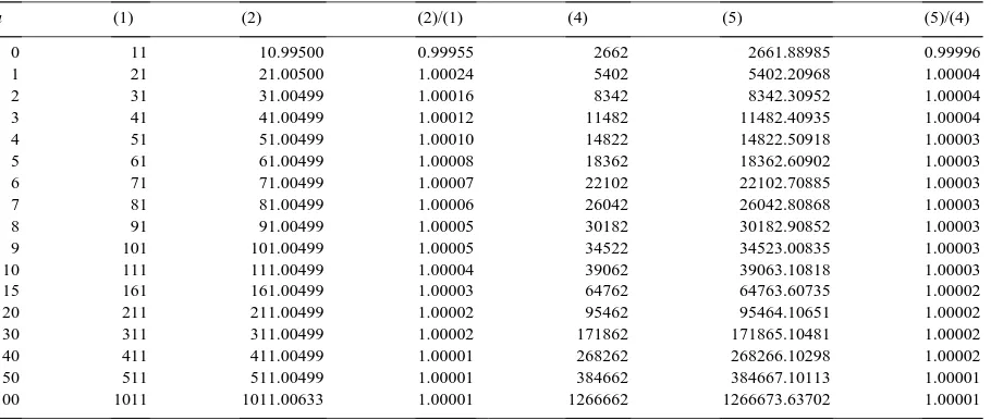
Table 1
First and second moments ofTcfor exponential claim size
u (1) (2) (2)/(1) (4) (5) (5)/(4)
0 11 10.99500 0.99955 2662 2661.88985 0.99996
1 21 21.00500 1.00024 5402 5402.20968 1.00004
2 31 31.00499 1.00016 8342 8342.30952 1.00004
3 41 41.00499 1.00012 11482 11482.40935 1.00004
4 51 51.00499 1.00010 14822 14822.50918 1.00003
5 61 61.00499 1.00008 18362 18362.60902 1.00003
6 71 71.00499 1.00007 22102 22102.70885 1.00003
7 81 81.00499 1.00006 26042 26042.80868 1.00003
8 91 91.00499 1.00005 30182 30182.90852 1.00003
9 101 101.00499 1.00005 34522 34523.00835 1.00003
10 111 111.00499 1.00004 39062 39063.10818 1.00003
15 161 161.00499 1.00003 64762 64763.60735 1.00002
20 211 211.00499 1.00002 95462 95464.10651 1.00002
30 311 311.00499 1.00002 171862 171865.10481 1.00002
40 411 411.00499 1.00001 268262 268266.10298 1.00002
50 511 511.00499 1.00001 384662 384667.10113 1.00001
100 1011 1011.00633 1.00001 1266662 1266673.63702 1.00001
and we can compare the approximations for these moments given by using the appropriate discrete model described earlier.
In Table 1 we show values for E[Tc|u] and E[Tc2|u] together with the respective approximating values
β−1E[Td∗|βu]/ψd∗(βu)andβ−2E[Td∗2|βu]/ψd∗(βu)for different values of initial surplusu. The key for the table is the following: (1) and (4) show the true values of E[Tc|u] and E[Tc2|u], (2) and (5) show the
approxima-tions for these quantities, respectively; columns 4 and 7 of the table show the ratios (2)/(1) and (5)/(4), respectively.
Example 2 (Combination of exponentials claim amounts). In this example we took a combination of two
ex-ponentials presented by Gerber et al. (1987, Section 5) which we rescaled to have mean 1. That is p(x) = 7 e−(7/4)x−7 e−(7/3)x,x≥0.
Following the method by Lin and Willmot (2000), and using a similar notation we get ψ(u) = −0.00952025 e−3.05264u+0.918611 e−0.121604u,E[Tc|u]=ψ1(u)/ψ(u)andE[Tc2|u]=ψ2(u)/ψ(u), where
ψ1(u) =e−3.17424u[e0.121604u(0.8221+0.000996986u)+e3.05264u(6.72892+9.28231u)], ψ2(u) =e−18.8022u[93.7952 e18.6806u(0.699241+u)(18.6476+u)
−0.000104407 e15.7496u(−609.786+u)(2255.98+u)].
Table 2 shows values for E[Tc|u] and E[Tc2|u] together with the respective approximating values
β−1E[Td∗|βu]/ψd∗(βu)andβ−2E[Td∗2|βu]/ψd∗(βu)for different values of initial surplusu. The key for this table is the same as in Example 1.
If we look at the approximating values and compare with the previous examples we see that they show a similar pattern, although not as good as before. It is readable that the algorithm show signs of instability for very high values of the initial surplus.
Example 3 (Erlang(2) claim amounts). In this example we consider a Gamma(2,2) claim amount distribution with
p.d.fp(x)=4xe−2x,x≥0.
Mathe-Table 2
First and second moments ofTcfor a combination of two exponentials claim size
u (1) (2) (2)/(1) (4) (5) (5)/(4)
0 8.30612 8.30112 0.99940 1503.30279 1503.21944 0.99994
1 17.48729 17.49228 1.00029 3419.11003 3419.28422 1.00005
2 27.53791 27.54290 1.00018 5691.23339 5691.50765 1.00005
3 37.63947 37.64445 1.00013 8176.60121 8176.97602 1.00005
4 47.74400 47.74899 1.00010 10866.72068 10867.19605 1.00004
5 57.84872 57.85370 1.00009 13761.08329 13761.65918 1.00004
6 67.95344 67.95842 1.00007 16859.65866 16860.33506 1.00004
7 78.05816 78.06314 1.00006 20162.44498 20163.22187 1.00004
8 88.16288 88.16786 1.00006 23669.44216 23670.31950 1.00004
9 98.26761 98.27259 1.00005 27380.65017 27381.62796 1.00004
10 108.37233 108.37731 1.00005 31296.06903 31297.14723 1.00003
15 158.89594 158.90091 1.00003 53936.32596 53937.90605 1.00003
20 209.41956 209.42450 1.00002 81681.85394 81683.93635 1.00003
30 310.46678 310.47160 1.00002 152488.72308 152491.82578 1.00002
40 411.51401 411.51840 1.00001 243716.67644 243720.91937 1.00002
50 512.56124 512.56420 1.00001 355365.71403 355371.72337 1.00002
100 1017.79737 1016.91321 0.99913 1219927.16536 1221303.49553 1.00113
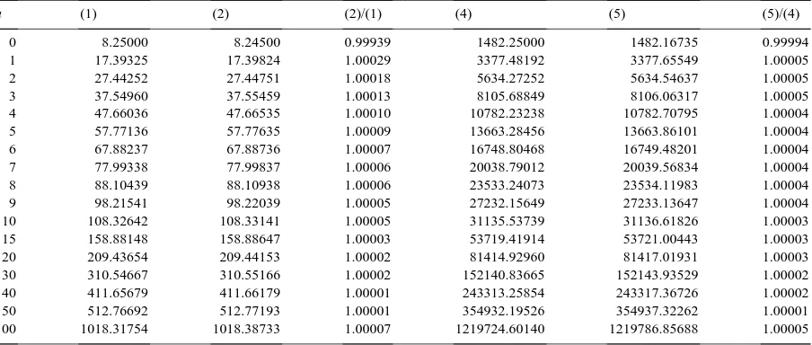
Table 3
First and second moments ofTcfor a Gamma(2,2) claim size
u (1) (2) (2)/(1) (4) (5) (5)/(4)
0 8.25000 8.24500 0.99939 1482.25000 1482.16735 0.99994
1 17.39325 17.39824 1.00029 3377.48192 3377.65549 1.00005
2 27.44252 27.44751 1.00018 5634.27252 5634.54637 1.00005
3 37.54960 37.55459 1.00013 8105.68849 8106.06317 1.00005
4 47.66036 47.66535 1.00010 10782.23238 10782.70795 1.00004
5 57.77136 57.77635 1.00009 13663.28456 13663.86101 1.00004
6 67.88237 67.88736 1.00007 16748.80468 16749.48201 1.00004
7 77.99338 77.99837 1.00006 20038.79012 20039.56834 1.00004
8 88.10439 88.10938 1.00006 23533.24073 23534.11983 1.00004
9 98.21541 98.22039 1.00005 27232.15649 27233.13647 1.00004
10 108.32642 108.33141 1.00005 31135.53739 31136.61826 1.00003
15 158.88148 158.88647 1.00003 53719.41914 53721.00443 1.00003
20 209.43654 209.44153 1.00002 81414.92960 81417.01931 1.00003
30 310.54667 310.55166 1.00002 152140.83665 152143.93529 1.00002
40 411.65679 411.66179 1.00001 243313.25854 243317.36726 1.00002
50 512.76692 512.77193 1.00001 354932.19526 354937.32262 1.00001
100 1018.31754 1018.38733 1.00007 1219724.60140 1219786.85688 1.00005
matica, as their expressions lead to infinite series. Table 3 shows values forE[Tc|u] andE[Tc2|u] together with
the respective approximating valuesβ−1E[Td∗|βu]/ψd∗(βu) andβ−2E[Td∗2|βu]/ψd∗(βu), produced by the pro-posed recursions, for different values of initial surplusu. The key for this table is the same as in the previous examples.
The approximating figures in this case show a similar accuracy when compared with the previous examples.
Acknowledgements
References
Delbaen, F., 1988. A remark on the moments of ruin time in classic risk theory. Insurance: Mathematics and Economics 9, 121–126. de Vylder, F., Goovaerts, M.J., 1988. Recursive calculation of finite time ruin probabilities. Insurance: Mathematics and Economics 7, 1–8. Dickson, D.C.M., Eg`ıdio dos Reis, A.D., 1996. On the distribution of the duration of negative surplus. Scandinavian Actuarial Journal 2,
148–164.
Dickson, D.C.M., Waters, H.R., 1991. Recursive calculation of survival probabilities. Astin Bulletin 21 (2), 199–221.
Dickson, D.C.M., Eg´ıdio dos Reis, A.D., Waters, H.R., 1995. Some stable algorithms in ruin theory and their applications. Astin Bulletin 25 (2), 153–175.
Eg´ıdio dos Reis, A.D., 1993. How long is the surplus below zero? Insurance: Mathematics and Economics 12, 23–38.
Gerber, H.U., 1974. The dilemma between dividends and safety and a generalization of the Lundberg–Cramér formulas. Scandinavian Actuarial Journal, 46–57.
Gerber, H.U., 1979. An Introduction to Mathematical Risk Theory. S.S. Huebner Foundation Monograph Series No. 8. Irwin, Homewood, IL. Gerber, H.U., 1990. When does the surplus reach a given target? Insurance: Mathematics and Economics 9, 115–119.
Gerber, H.U., Goovaerts, M.J., Kaas, R., 1987. On the probability and severity of ruin. Astin Bulletin 17 (2), 151–163 .
Lin, X.S., Willmot, G.E., 2000. The moments of the time of ruin, the surplus before ruin, and the deficit at ruin. Insurance: Mathematics and Economics 27, 19–44.
Panjer, H.H., 1981. Recursive calculation of a family of compound distributions. Astin Bulletin 12 (1), 22–26.