International Review of Economics and Finance 9 (2000) 123–137
Initial beliefs and the global stability of least
squares learning
M. C. Chang
a, C. Y. Cyrus Chu
b,c, Kenneth S. Lin
b,*
aGraduate Institute of Industrial Economics, National Central University, Chung-li, Taiwan
bDepartment of Economics, National Taiwan University, Taipei, Taiwan
cInstitute of Economics, Academia Sinica, Taipei, Taiwan
Received 20 January 1998; accepted 31 March 1999
Abstract
This article provides an operational framework of global stability analysis when Ljung’s (1977) ordinary differential equation (ODE) approach is applied to the recursive stochastic system. We first establish the notion of stable set under which sufficient conditions for the equivalence between them can be translated to restrictions on initial beliefs in agents’ forecasts. The maximum ODE-stable set is simply the largest range of initial beliefs. We then demonstrate how to implement this operational framework for the analysis of stability beyond the local sense in some well-known models in the learning literature. 2000 Elsevier Science Inc. All rights reserved.
JEL classification:D83
Keywords:Least squares learning; Global stability; Initial belief
1. Introduction
Many recent researchers applied Ljung’s (1977) ordinary differential equation (ODE) approach to study the convergence of the least squares learning mechanism.1
When a model satisfies Ljung’s regularity conditions, the local stability of the recursive stochastic system generated by the learning mechanism would be governed by a simpler ordinary differential equation system. However, one drawback of this approach is that the stability of least squares learning mechanism beyond the local sense is difficult to analyze. As Marcet and Sargent (1989a, p. 360) pointed out, sufficient conditions
* Corresponding author. Tel.:102-2341-8190.
E-mail address: [email protected] (K.S. Lin)
124 M.C. Chang et al. / International Review of Economics and Finance 9 (2000) 123–137
for global convergence are “much more difficult to analyze in cases where agents include endogenous variables among their regressors.”
In this article, we propose an operational framework of global stability analysis when Ljung’s ODE approach is adopted. We first establish the notion of stable set under which sufficient conditions for the equivalence between the recursive stochastic system and corresponding ordinary differential equations can be translated to restric-tions on initial beliefs in the perceived law of motion for agents’ forecasts. The
maximum ODE-stable set is simply the largest range of initial beliefs so that one can use Ljung’s ODE approach to obtain the stability of the least squares learning mechanism beyond the local sense. The explicit characterization of the maximum stable set is important and useful since it helps us understand the empirical significance of the least squares learning mechanism, and recognize the justifiable range of compar-ative statics.
We will demonstrate that the maximum ODE-stable set is characterized by the combination of the following three conditions: (1) the autoregressive coefficient matrix in the state variable transition rule must have eigenvalues all less than one in modulus; (2) the state variables must be bounded infinitely often with probability one; and (3) the differential equations which govern the original stochastic difference equations must be stable in the relevant range. Each of these three conditions places restrictions on initial beliefs in the perceived law of motion for agents’ forecasts. If the maximum stable set turns out to be a universal set, then the learning mechanism under study is globally stable.
To establish the equivalence between the stability of difference equation system and that of differential equation system, we need regularity conditions governing the evolution of parameters in agent’s forecasts. For instance, as argued in Ljung (1987, p. 57), any approach (such as the ODE approach and the martingale approach) that describes the behavior of a recursive stochastic system with the “small step” techniques requires the boundedness of state variables in the system as described in the second condition. Otherwise, the equivalence between the solution of this system and the trajectory of corresponding ordinary differential equations can be easily destroyed by an immediate jump of parameters in agents’ forecasts. Further, because any stochastic mechanism using small step techniques does not have its own mechanism to keep relevant parameters on a desirable region, we also need an auxiliary facility that projects diverging parameters in agents’ forecasts back to the region. In this article, we demonstrate that even if the differential equation system is globally stable, it is alway possible to find the projection facility that interferes with the trajectory of differential equation system. Thus, without appropriate regulations on the projection facility, the traditional definition of global stability cannot be operational.
2. The stability beyond the local sense: A general framework
LetztPRk be ak 31 the state vector of the economic system. The actual law of motion forztis assumed to follow the linear stochastic difference equation:
zt5A(bt)zt211B(bt)ut, (1)
whereutis anm31 vector white noise that is orthogonal to zt2jfor j .0, A(bt) and
B(bt) are matrices with the dimension k 3k and k3 m, respectively. Letz1tPRk1
and z2t P Rk2 be subvectors of zt. Here z1t and z2t are, respectively, those variables whose future values agents care about and those used by agents to predict future values ofz1t. At timet, suppose agents believe thatz1,t11evolves according toz1,t115
z92tb1vt11, wherevt11is a vector white noise orthogonal toz2t. Letbtbe the estimate
ofbat timet.The role of economic theory is to induce the mappingA(bt) andB(bt), which determine the actual law of motion for the forecast ofz1,t11.
For a given set of perceived values of b, it is possible to use the actual law of motion [Eq. (1)] to deduce the least squares projection of z1,t11onz2t:
Eˆ[z1,t11|z2t] 5z92tT(b),
whereT(b) is determined by the least squares learning mechanism. A rational expecta-tions equilibrium is a stationary point of the mappingT(b)→ b, denotedbf.
2.1. The ODE approach
As agents use the least squares mechanism to learn about the actual law of motion, their belief (bt) evolves according to the following recursive formula:
bt5 bt211
at
tR
21
t21z2,t21[z91,t212z92,t22bt21], (2a)
Rt5 Rt211
at
t
3
z2,t21z92t212 Rt21at
4
, (2b)in which at is a non-decreasing weight sequence of positive real numbers and Rtis the estimate of the second moment ofz2tat timet.When the value of (bt, Rt) generated
from the recursive formulas falls outside the set of reasonable values (D1), agents
project the observed vector (bt,Rt) onto a most likely region (D2). Formally, the
projection facility can be described as
(bt, Rt) 5
5
some point in(bt,Rt), D if (bt, Rt) PD1,2, otherwise. (2c)
To apply Ljung’s ODE approach, we need to assume thatD1is an open bounded set
containing the compact set D2(Ljung, 1977, Theorem 4) throughout this article.
The use of Ljung’s ODE approach in the study of the limiting behavior ofbtand
Rtrequires the mechanical transformation of the stochastic difference equations into the approximating ordinary differential equations:
3
b˙ (t)R˙(t)
4
53
R(t)21M(b(t))[T(b(t)) 2 b(t)]
126 M.C. Chang et al. / International Review of Economics and Finance 9 (2000) 123–137
in which y˙(t) ; dy(t)/dt and M(b) 5 E[z2t(b)z2t(b)9]. Here and henceforth, let y(t)
denote the variable generated by an ordinary differential equation, and yt the one generated by the corresponding stochastic difference equation. SinceM(b) is positive semi-definite for all t, R(t) is positive definite so long asR(0) is positive definite.
LetRf 5M(bf) andDAbe a domain of attraction of (bf,Rf), a stationary point of Eq. (3). According to Ljung (1977, p. 567), if DA is not a singleton set, then there exists a Lyapunov function with the following properties:
b1. V(b,R) is infinitely differentiable,
b2. 1.V(b, R) $0 for any (b,R) PDA and V(bf,Rf) 50, and
b3. when evaluating along the solution of Eq. (3), dV(b(t), R(t))/dt # 0 for any (b(t), R(t)) PDA, and the equality holds only when (b(t), R(t))5 (bf, Rf). According to Hartman (1973, p. 548), if (bf, Rf) is a unique stationary point and is locally stable, then DA is an open set so long as the domain of ordinary differential equation is open.
The central proposition of least squares learning convergence can be stated as follows, which is a slight variation of Theorem 4 in Ljung (1977):
Proposition 1. Let (bt,Rt) be generated by the learning mechanism Eqs. (1) and (2). Suppose the five regularity conditions a1–a5 given in Appendix 1 hold. If
c1. ztis bounded infinitely often with probability one, and
c2. (bf,Rf)PD2,D1,DA, (bf,Rf) is not on the boundary ofD2, and there
exists a Lyapunov function with properties b1–b3 such that V(ba, Ra) .
V(bb,Rb) for any (ba, Ra) Ó D1and (bb,Rb) PD2,
then (bt, Rt) →(bf, Rf) almost surely ast→ ∞.
Proposition 1 states that the limiting behavior of (b(t), R(t)) in (3) mimics the limiting behavior of (bt, Rt) in Eq. (2) under certain conditions. Notice that the sets
D1 and D2 regulate the evolution of bt and Rt in the stochastic difference equation, while the maximum domain of attraction DA determines the trajectory of b(t) and
R(t) in the ordinary differential equation.
2.2. The problem with the traditional definition of global stability
Three things have to be accomplished in the stability analysis of the least squares learning mechanism using Ljung’s ODE approach. First, we have to obtain a set of restrictions on initial beliefs in which zt is bounded infinitely often with probability one. Second, we have to find the largest domain of attraction of the stationary point of Eq. (3), (bf,Rf). Third and most importantly, we have to have a projection facility 2c so that the equivalence between the stochastic difference equations, Eqs. (2a)–(2c), and the ordinary differential equations, Eq. (3), can be preserved.
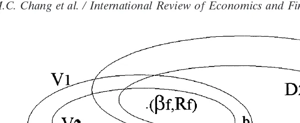
It is the projection facility that often blurred the notion of global stability. The following example can illustrate our point. Even thoughD1andD2usually cannot be
Fig. 1. The domain of attraction and projection facility.
The learning mechanism is said to be globally stable if (bt, Rt) → (bf, Rf) for any bounded open set D1 and any compact set D2 such that D2 ,D1. Imagine that the
solution of the ordinary differential equations in Eq. (3) is globally stable and V(b,
R) is a Lyapunov function. As shown in Fig. 1, we can always find D1 and D2 such
that D2 ", V1?0/ and V2 ", D1 ?0/, in which V1 5{(b, R)|V(b, R) , c1} and
V2 5 {(b, R)|V(b, R) , c2} with 0 , c2 , c1. Consider a point in D2, say b. The
trajectory of differential Eq. (3) may move pointb to point a.This movement leads to a value of Lyapunov function less than that in b, whereas point a following the learning mechanism [Eq. (2)] will be projected back toD2. That is, even if the
differen-tial equations system is globally stable, it is always possible to find a pair ofD1and
D2such that the projection facility interferes with the trajectory of ordinary differential
equations. As a result, the trajectory of Eq. (3) no longer mimics that of the learning mechanism characterized by Eq. (2).2Thus, without further restricting the ranges of
D1and D2, the above definition of global stability is not operational.
2.3. An operational definition of global stability
To assure the legitimate correspondence between the ordinary differential equation system [Eq. (3)] and the stochastic difference equation system [Eq. (2)], we must impose further restrictions on the setsD1and D2:
Definition 1: Consider the system Eq. (1) and Eq. (2), and the ordinary differential equations, Eq. (3) with the largest domain of attraction DA. Further, consider a connected setDwhich contains (bf,Rf) and is a subset ofDA. If for any neighborhood of (bf,Rf) denoted 1(bf,Rf) which is bounded and connected, and whose closure is contained in D, there exist D1 . 1(bf, Rf) and D2 . 1(bf, Rf) such that (bt, Rt)
converges to (bf, Rf) almost surely,3then D is called anODE-stable set for Eq. (1)
and Eqs. (2a)–(2b).
This definition states that whenDis an ODE-stable set, it is certain that there is a projection facility which guarantees the almost sure convergence of the estimate andD2is “large” enough so that it can approximateD.How economic agents choose
128 M.C. Chang et al. / International Review of Economics and Finance 9 (2000) 123–137
do is to specify the range in whichD1andD2can be chosen appropriately to guarantee
the stability of learning mechanism.
Dmust be restricted to be contained inDA, for otherwise the ordinary differential equations in Eq. (3) are unstable, which is clearly incompatible with the logic of ODE stability. If the focus is on the local stability of Eq. (3), then the use of Eq. (3) is restricted to the stability analysis of Eqs. (2a)–(2b) in the local sense. Only when Eq. (3) has a “more-than-local” domain of attraction can we use the ODE approach to discuss the stability of the learning mechanism in the large. The initial condition (b0,
R0) does not appear in the above definitions because the projection facility Eq. (2c)
could project the outlying point (b0, R0) back to D2.
Definition 2: D*,DAis called themaximum ODE-stable setif it is an ODE-stable set, and any other ODE-stable set is contained inD*.
Definition 3: A learning mechanism is called ODE globally stable if D* is the universal set.
The empirical relevance of the maximum ODE-stable set can be interpreted as follows. Suppose that an ODE-stable setD is very small, then the legitimate range whereD1andD2can be chosen is much restricted. Therefore, we do not expect that
economic agents can perceive D1 and D2 accurately, and the ODE-stability of the
learning mechanism cannot be assured.
The following proposition gives us the conditions which should be verified for a ODE-stable set.
Proposition 2: If regularity conditions a1–a4 in Appendix 1 are satisfied, and if the following conditions hold:
a5. the characteristic roots of A(b) are all less than one in modulus for (b,
R) PD, DA, and
c1. for any compact subset of D denoted Db, if (bt, Rt) P Db for all t, zt
generated by Eq. (1) is bounded infinitely often with probability one,
thenDis an ODE-stable set.
Proof: Because DA is a domain of attraction of (bf, Rf) for Eq. (3), there is a Lyapunov function V(b(t), R(t)) satisfying b1–b3. Consider a neighborhood of (bf,
Rf) denoted 1(bf, Rf), whose closure is entirely in D. We first select a connected compact setD2such that 1(bf,Rf),D2,D, and then pickD15{(b,R)|V(b,R) ,
k} in which max D2
V(b, R) ,k, 1.
According to properties b2 and b3 ofV(b,R), maxD2V(b, R),1, which guarantees the existence ofk. Under the above choice ofD1andD2, condition c2 in Proposition
1 is satisfied, and hence Proposition 1 applies,QED.
It follows from the proof that ifDis an open ODE-stable set then the closure of
to the regularity conditions listed in the Appendix 1, most of them are not particularly important in our discussion. Specifically, a2 and a4 are not related to the parametric specification of the model and a1 and a3 cannot be violated for a well-behaved economic system. Thus, what remain to be verified are c1 and a5. This is why in Proposition 2 we explicitly single out a5 and c1 to emphasize that these two conditions are the ones need to be verified in applications.4
2.4. A scalar parameter case
If the focus is on the local stability of the learning mechanism, Marcet and Sargent (1989a) show that the local stability of Eq. (3) is determined by the simpler differential equation:
b˙ (t) 5 T(b(t))2 b(t). (4) The advantage of studying Eq. (4) is that it has fewer dimensions and therefore is easier to analyze than Eq. (3). However, the local connection between the characteristic roots of Eq. (3) and those of Eq. (4) does not necessarily establish the connection between the domain of attraction for Eq. (3) and that for Eq. (4), which is necessary for the global stability analysis. The following proposition establishes that, when bt is a scalar, the domain of attraction for the simpler differential equations of Eq. (4) determines those of Eq. (3).
Proposition 3: Consider the systems Eq. (3) and Eq. (4) in whichb(t) is a scalar. If there is a domain of attraction ofbfdenotedDA(b)for the ordinary differential
equation Eq. (4), then DA(b)351 is the domain of attraction of (bf,Rf) for the
ordinary differential equations Eq. (3).
Proof: Since DA(b) is the domain of attraction of bf for Eq. (4), there exists a Lyapunov functionV(b(t)) with properties similar to b1–b3. More specifically, when evaluated along the solution path of Eq. (4), we have
dV(b(t))/dt5 V9(b(t))[T(b(t))2 b(t)] #0, ∀b(t) PDA(b).
The equality holds only when b(t) 5 bf. Now we want to search for a Lyapunov functionW(b(t), R(t)) for Eq. (3). It is natural to try
W(b(t), R(t)); V(b(t)).
Then we check whether theW(·, ·) function so defined is a Lyapunov function of Eq. (3). Suppose that (b(t), R(t)) is the trajectory of Eq. (3) and (b(t), R(t)) P DA(b) 3
51. Then we see that
dW/dt;dV(b(t))/dt5V9(b(t))R(t)21M(b(t))[T(b(t))2 b(t)]#0.
The above inequality holds becauseM(b).0 andR(t)21.0 by assumption, and the
equality holds only whenb(t) 5 bf. This shows that the Lyapunov functionV(b(t)) for the differential equation Eq. (4) determines the convergence of (b(t),R(t)) to (bf,
130 M.C. Chang et al. / International Review of Economics and Finance 9 (2000) 123–137
(3) starting from DA(b) 3 51 will eventually fall inside {(bf, R):R . 0}. Once this
happens, it is easy to see that (b(t), R(t))→(bf, Rf) as t→∞; QED.
3. Deriving the maximum stable set: Some examples
We show in Proposition 2 that the maximum ODE-stable set is in fact the intersection of three regions. Specifically, we need to see (1) when the autoregressive coefficient matrixA(·) in Eq. (1) have all its eigenvalues less than one in modulus (condition a5 in Appendix 1); (2) when the parameters of the model can bound the state variables infinitely often with probability one (condition c1 in Proposition 1), and (3) when the differential equations which govern the original stochastic difference equations are stable (implicit in the condition D , DA). Each of these three conditions imposes restrictions on initial beliefs on relevant parameters in agents’ forecasts. In what follows we show how to derive the ODE-stable set in some well-known models in the learning literature.
3.1. Cagan’s model: A case of an endogenous variable as one of regressors
We first study a stationary version of Cagan’s (1956) inflation model with endoge-nous money supply, which consists of:5
pt5 lEtpt111 mt, (5)
mt5 rmt212 gpt211ut. (6)
Eq. (5) and (6) are the demand function for real cash balance and the money supply rule, respectively.l . 0 implies that the rising opportunity cost of holding cash due to risingEtpt11decreases agents’ demand for real cash balance. The information set
at timet in Eq. (5) includesmt, and all lagged values of mtand pt. Wheng . 0, the monetary authorities adopt a counter-cyclical monetary policy: the authorities decrease current money supply as a response to an increase in price level in the previous period.6
Suppose agent formulates his forecast ofpt11at time taccording toEtpt115 btmt.
Substitutingbtmt into Eqs. (5) and (6) yields the following actual law of motion for
pt: pt 5 r(lbt1 1)mt212 g(lbt 11)pt21 1(lbt11)ut. For a given estimate ofb, we can use the actual law of motion ofptto deduce the linear least squares projection of pt11: Eˆ[pt11|mt] 5 (lb 1 1) [r 2 g (lb 1 1)] mt, which can be expressed as the
operator for the learning mechanism:
T(b) 5(lb 1 1)[r 2 g(lb 11)].
Substituting the perceived law of motion ofptinto Eq. (6) for pt21yields
mt5[r 2 g(lbt211 1)]mt211ut.
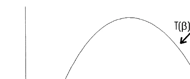
Fig. 2. The maximum domain of attraction ofbf.
{b||r 2 g(lb 1 1)| ,1} (7)
is one of the three regions we are looking for. Notice that the two characteristic roots ofA(b) in Eq. (3) are 0 andr 2 glb 2 g. Let Dd(b)be
Dd(b);
5
b|1
b 2r 2 g 2 1 lg
2 1
b 2r 2 g 1 1 lg
2
,06
.It is easy to see that if g . 0 and b P Dd(b), then the regularity condition a5 in
Appendix 1 is satisfied. Further, in view of Eq. (7), b P Dd(b) also guarantees the
boundedness ofmt.
Next we need to find the domain of attraction for the corresponding ordinary differential equation. For a scalar case of bt, Proposition 3 in Section 2 shows that the stability is governed by the following ordinary differential equation:
b˙ 5T(b)2 b 5 (lb 1 1)[r 2 g(lb 1 1)] 2 b.
It is easy to verify thatT″,0, and thereforeT(b)2 bshould look like Fig. 2. There are two stationary points of the mappingT(b) →b, but we find that only
bf(g,r, l) 5
√
(lr 2 1)214lg 1 lr 2 2lg 2 1
2gl2 ,
is the possible candidate of equilibrium.7It is clear from Figure 2 that the maximum
domain of attraction of bf is DA(b) 5 {b|b . b9f(g, r, l)}, which, by Proposition 3, implies thatDA(b)351is the maximum domain of attraction. Hence, the maximum
stable set is the intersection of {(b, R)|bPDd(b)} and DA(b)351.
Finally, it is interesting to see that the range of the open intervalDd(b)is decreasing
132 M.C. Chang et al. / International Review of Economics and Finance 9 (2000) 123–137
3.2. Frydman’s model: A case of global stability
Here we study a Marcet and Sargent’s (1986) two-firm version of Frydman’s (1982) model. This example illustrates that the learning mechanism can be easily verified as globally stable when agents use only exogenous variables to forecast equilibrium price level. Suppose there are two competitive firms indexed byi51, 2. Demand for the firm’s output is assumed to bept 5a 2 b
o
2i51hit 1 et, in which a, b . 0, hit is theoutput of firmi, and etis an i.i.d. random variable. Firmi’s cost function at timetis
C(hit) 5(s/2)(hit)21kithit1c, where cand s are positive parameters, andk
the error term vector. It can be shown that the actual law of motion for price can be expressed in the form of Eq. (1)9, where A(bt) is a 333 zero matrix, andB(bt) is
3
a 2bso
2i51b1it 2bs[o
2i51(bi2t21)] 1 2bs(b12t21) 2bs(b22t21)0 1 0 1 0
0 1 0 0 1
4
.Because A(bt) is a zero matrix and B(bt) is bounded for bt in any compact set, we see that the characteristic roots ofA(bt) are all zeros for all possible values ofb, and thatztis bounded infinitely often with probability one under the i.i.d. assumption of
ut.10As such, the stability property of this model hinges upon the domain of attraction
of the differential Eq. (3).
with l 5 [Var (dt)]/[Var (dt) 1 Var (et)]. bf is a rational expectations equilibrium if b1 independent ofb. Thus, the stability property of Eq. (3) is this model can be derived by studying the simpler differential equationb˙ (t) 5T(b (t)) 2 b(t), whereT(b) 5 (T1(b), T2(b)). We find that the four characteristic roots of the derivative ofT(b) 2
In the above discussion, we find that the fulfillment of the sufficient conditions in Proposition 2 does not need any additional restrictions, so the maximum stable set is a universal set and the learning mechanism is globally ODE-stable.
3.3. Bray’s model: Using Lyapunov function to find the maximum stable set
Bray (1982) studied a model in which there areNi.0 informed traders andNu. 0 uninformed traders. Both types of traders observe market price pt at time t, and the return on the asset rt at a date after t but before t 1 1. Further, the informed traders are assumed to observe the exogenous supply of the asset,st. Both rt and st are i.i.d. random variables, satisfying the following relationship: rt 5 E[rt] 1 r(st 2
E[st])1 et, in which Eis the expectation operator, r 5cov(rt, st)/var(st), andet is a white noise process orthogonal tost.
The demand for the asset by informed agents at timetisui[E[rt|st]2pt],ui.0, in whichE[rt|st]5E[rt]1 r(st2E[st]). The uninformed agents useptin forming their expectations of rt at timet: E[rt|pt] 5 b11 b2pt, which determine their demand for
the asset:uu[E[rt|pt]2pt] withuu.0. Letb5(b1,b2)9andbt5(b1t,b2t}9. The estimate
ofb at timet (bt) is determined by Eqs. (2a)–(2b) withz2t5 (1,pt)9 and z1t5rt21.11
Ifvar (st) .0, then the least squares projection of rton z2tis given by Eˆ[rt|z2t] 5z92t
T(b), in which
T(b) 5
3
E[rt] 2k(NiuiE[rt] 2E[st])/Nuuu 2kb1k(Niui1Nuuu)/Nuuu 2kb2
4
,
withk 5Nuuu/(Niui2 r21). It is straightforward to show that if k ?21, then there
is a unique stationary point ofT(b) →b:
bf 5
3
[E[rt] 2 k(NiuiE[rt] 2 E[st])/Nuuu](1 1k) 21k(Niui 1Nuuu)/(11k)Nuuu
4
.It can be shown that the learning mechanism is locally stable (unstable) ifk . 21 (k , 21). Therefore, it is assumed thatk . 21.
Letzt5 (pt, rt, st)9 and ut5 (rt, st, 1)9. It is easy to see that the coefficient matrix
A(bt) in Eq. (1) is a 333 zero matrix and hence the regularity condition a5 is satisfied in this model. Therefore, the limiting behavior of (bt, Rt) can be approximated by that of (b(t),R(t)). However, it is hard to study the stability of this learning mechanism beyond the local sense sinceptused as a regressor in forming the uninformed agents’ expectation of rtis an endogenous variable. In what follows we shall show that the global stability of the learning mechanism can be studied directly, without having to analyze the simpler differential equation in Eq. (4) as a bridge. This is a step beyond the contribution of Marcet and Sargent (1989a).
We first show that expectation of the squared prediction error is a Lyapunov function for the differential equation system of Eq. (3). ConsiderV(b(t))5(1/2)E[et(b(t))]2, in
whichet(b(t)); rt2z2t(b(t))9b(t) is the prediction error. When evaluated along the
134 M.C. Chang et al. / International Review of Economics and Finance 9 (2000) 123–137
d
dtV(b(t)) 5 2E[l(b(t))z2t(b(t))et(b(t))]9 R(t)
21 E[z2t(b(t))et(b(t))], (8)
in which
l(b) 5 Nuuu 1Niui
Nuuu(12 b2) 1Niui
.
According to Eq. (8), ifR(t) is a positive definite matrix andl(b) .0 (that is,b2,
(Niui 1 Nuuu)/Nuuu), then (d/dt)V(b(t)) # 0 and the equality holds when b(t) 5 bf. Thus, the maximum domain of attraction of (bf,Rf) is12
DA 5{(b,R)|b2 ,(Niui1Nuuu)/Nuuu, Ris a positive definite matrix}.
It is clear from the assumption ofk. 21 thatb2f,(Niui1Nuuu)/Nuuu, which implies
(bf,Rf) PDA. Finally, because a1–a5 are always satisfied in Bray’s (1982) model, DA
is also the maximum ODE-stable set for the learning mechanism.
4. Conclusions
The purpose of this article is to propose an operational definition for the global stability of least squares learning. Knowing the range of stability in the large can help us understand the empirical relevance of the convergence of least squares learning, and determine the justifiable range for comparative static analysis. There are some elements we note as we search for such a definition: (1) The two setsD1and D2 in
the projection facility cannot be arbitrarily chosen, for otherwise the ODE approach will not apply. (2) Within the largest domain of attraction for the ordinary differential equation system, ifD1andD2are appropriately chosen, the learning mechanism will
almost surely converge. (3) To find the maximum stable set, the most important criteria we have to check are the (infinitely often) boundedness of the state variable, and the conditions that warrant the regularity condition a5. (4) Only when the maxi-mum ODE-stable set turns out to be the universal set can we say that the learning mechanism is globally stable. We also demonstrate how to derive such maximum stable sets in three well-known economic models in the learning literature, in which only one of them is globally stable.
Acknowledgments
We thank Professors L. Ljung of Linko¨ping University, Sweden and Chung-Ming Kuan of National Taiwan University, Taiwan and three referees for helpful suggestions and comments.
Notes
et al. (1995) pointed out and corrected two types of errors in Marcet and Sargent’s analysis.
2. See Ljung (1977, p. 557) for the detailed discussion.
3. It is equivalent to state that D2 , D1 , DA, and Eqs. (1) and (2) can be
legitimately approximated by Eq. (3).
4. In view of Proposition 1, Proposition 2 essentially states that within D,DA, one can always find D1and D2such that c2 is satisfied.
5. A similar specification of money supply process was used in McCallum (1983). 6. Both Cagan (1956) and Marcet and Sargent (1989b) considered the exogenous
money supply with g 5 0. our analysis. Finally, when g 5 0, there is a unique solution of T(b) 5 b: r/ (12 lr).
8. It can be verified that the lower (upper) bound of open interval [(r 2 g 21)/ (lg), (r 2 g 11)/(lg)] decreases (increases) withg. Sincebf(g,r,l) intersects [(r 2 g 11)/(lg)] at the point g 5(r 1 1)(l 1 1),g ,(r 11)(l 1 1) must hold to guarantee the validity of a5. This restriction, however, is irrelevant to our stability analysis. The rest of the derivation is straightforward.
10. The proof is similar to that of the lemma in Appendix 2.
136 M.C. Chang et al. / International Review of Economics and Finance 9 (2000) 123–137
12. Sincel(b) is discontinuous when b 5 (Niui1Nuuu)/Nuuu, DA is the whole set which contains (bf,Rf) and is connected, and in which the differential equation is defined. As shown in Ljung and So¨derstro¨m (1983, pp. 149–150), if DA is such a whole set, then the Lyapunov function V(b(t)) does not require that
V(b(t)),1 in b2 be satisfied.
References
Bray, M. (1982). Learning, estimation, and stability of rational expectations.Journal of Economic Theory, 26, 318–339.
Cagan, P. (1956). The monetary dynamics of hyperinflation. In M. Friedman (Ed.),Studies in the Quantity
Theory of Money(pp. 25–117). Chicago: University of Chicago Press.
Chang, M. C., Chu, C. Y. C., & Lin, K. S. (1995). A note on least-square learning mechanism.Journal
of Economic Dynamics and Control 19, 1293–1296.
Frydman, R. (1982). Toward an understanding of market process.American Economic Review 72, 652–668. Hahn, W. (1967).Stability of Motion.Berlin, Germany: Springer-Verlag.
Hartman, P. (1973).Ordinary Differential Equations(2nd ed.). New York: John Wiley and Sons, Inc. Ljung, L. (1977). Analysis of recursive stochastic algorithms.IEEE Transactions on Automatic Control
AC-22(4), 551–575.
Ljung, L. (1987). Recursive stochastic algorithm: ordinary differential equation methods. In M.G. Singh (Ed.),Systems and Control EncyclopediaNew York: Pergamon Press.
Ljung, L., & So¨derstro¨m, T. (1983).Theory and Practice of Recursive Indentification.Cambridge, MA: M.I.T. Press.
Marcet, A., & Sargent, T. J. (1986). Convergence of least squares learning in environments with hidden state variables and private information. Unpublished manuscript.
Marcet, A., & Sargent, T. J. (1989a). Convergence of least squares learning mechanisms in self-referential linear stochastic models.Journal of Economic Theory 48, 337–368.
Marcet, A., & Sargent, T. J. (1989b). Least-square learning and the dynamics of hyperinflation, in W.A. Barnett, J. Geweke, & K. Shell (Eds.),Economic Complexity: Chaos, Sunspots, Bubbles, and
Nonlinearity(pp. 119–137). Cambridge: Cambridge University Press.
McCallum, B. T. (1983). On non-uniqueness in rational expectations models.Journal of Monetary
Eco-nomics 11, 139–168.
Appendix 1: Five regularity conditions for the ODE approach
a1. A(b) andB(b) are continuously differentiable forb. a2. {at} is a real positive weight sequence with the limit a. a3. The covariance matrixM(b) is non-singular.
a4. utis a vector white noise process. Further, for each element of ut, denoteduit,
E|uit|p, ∞for allp .1.
a5. The characteristic roots of A(b) are all less than one in modulus.
Appendix 2: Infinitely-often boundedness of first-order Markov processes
Lemma: Consider a first-order Markov process of the scalar xt:
in which vtis an i.i.d. random variable. If there exists a positive constant c and 0 , l ,1 such that
|
p
t
i5j11
ai|, c· lt2j,
for any iand t, and htis bounded, then xtis bounded infinitely often with probabil-ity one.
Proof: Recursive substitutions givext5
o
tj51(p
t
i5j11ai)hjvj. So there exists a positive constantc1such that
|xt|#c1c
o
t
j51
lt2j|v j|.
Let i.o. denote infinitely often, the following inequalities hold:
1 $P(|xt|, k i.o.) $P(c1c
o
t
j51
lt2j|v
j|,k i.o.) 5P(yt#
k c1c
i.o.),
in whichyt5 lyt211|vt|. Here we want to show thatP(yt#k/(c1c) i.o.)51. Because
vtis an i.i.d. process, we have 1
n
o
n
i51
yi→a almost surely,