M00316

1 DIFFICULTY IN OPTIMIZATION FUNCTIONS

OF MATLAB AND HOW TO ANALYZE H.A Parhusip

Center of Applied Science and Mathematics Universitas Kristen Satya Wacana

Jl. Dipenegoro 52-60, Salatiga, 50711, Central Java Telephone number : 0062-298-321212 Email address : hannaariniparhusip@ yahoo.co.id

Abstract

This paper presents an example of using optimization function in MATLAB. The used data is considered as a smooth function of 3 variables. Unlike in a literature, one needs to design a smooth function in order to start with an optimization. After the parameters are obtained the optimization is employed to obtain the minimizer. The obtained objective function is noncoercive. Therefore the minimizer is obtained by solving the nonlinear system of the Lagrangian function which is constructed as a perturbed objective function. The optimizer can not be considered as the best solution since the Hessian is not positive definite.

Keywords : noncoercive function, Jacobian, least square, Hessian, singularity

Introduction

Understanding output of MATLAB’s program is not an easy task. After using any functions in MATLAB correctly, one needs to relate with an expected result. Therefore theoretical background that may be used in the functions must be known.

subjects and students could not also describe formally mathematical reasons in the given output by MATLAB.

There are many authors addressed on developing the MATLAB code for a particular purposes. For data single directional (azimuthal) in geosciences for instance, Jones [1] proposed a MATLAB script since for this special purpose one may not have the related function from the standard MATLAB Toolbox. The lsqnonlin (one of optimization functions in MATLAB) can not be used for the directional azimuthal data. The given data is shown in Table 1. The goal of this measurement is to identify the maximum protein that can be obtained from various observations.

Table 1

The used data for the optimization study (Observed by. Y.Martono at Lab. Chemistry, SWCU,2011)

(B)

Percentage of yeast

(Y)

Protein Day

1

Protein Day

2

Protein Day

3

Protein Day

4

1 5 0.714 0.75 1.76 3.22

1 7.5 1.33 1.88 0.21 1.33

1 12.5 0.88 1.38 0.93 2.38

Reseach Method

3 

 t B Y B

Y t

P 

          

 _{, , , unknown parameters (1)}

Note that we have made data into dimensionless to proceed futher computations. Using the standard least square means that we have to

minimize the residual function

2

1 ,



_ 

  

  

    

  

      n

i

i i i da ta

i t

B Y P

R 



.

Following the standard optimization to find the critical x* [,]T

means that we have to solve the system obtained by R: g(x)0. In more details, this leads to solve 0

 R

and 0

 



R

simultaneously,i.e

0 ) , ( : ln

ln 2 ₁

2

1 1

,   

   

           









  

  



g B Y t

B Y B

Y t B Y P

i i i

n

i i

i i

i i n

i i

i d a ta

i ; (2a)

0 ln

ln 2

2

1 1

,  

    

  









 i i

n

i i i i

i n

i i

i da ta

i t t

B Y t

t B Y

P 

 



:=g₂(,)=0. (2b)

Any algorithm with an iterative procedure requires an initial

guesses of solutions. There are several well-known algorithms such as

Newton-method, Broyden method, trust-region and using evolutionary

algorithm [2]. The last algorithm transforms the system of equations into

a multi-objective optimization problem. The ill-posed nonlinear

equations may also occur. Buong and Dung [3] have provided a

theoretical study on this particular problem by doing a regularization on

the problem which based on Tikhonov regularization method. However

the problem was designed in the variational form which was too much

standard Newton method. The Newton method solves a general system 0 ) (    x

g with a formula



( ( ))



1 ( ( )) )

( ) 1

(k k k k

x g x

g x

x          (3)

which provides a nonsingularity of matrix Jacobian g(x(k)) on each iteration step. The formula (3) is employed to Eq. (2a)-(2b) by deriving their derivatives manually each term on these equations. Therefore one needs ) , ( ) ( ) ( ) ( 2 2 1 1 ) ( k k x g g g g k x g                        

  (4)

with __g1₌ 

            



 2 1 , ln i i i n i i i da ta i B Y t B Y P   2 2 2 1 ln 2            



_ i i i n i i i B Y t B

Y  _{ ,}



 g1 ₌

i i i i n i i i i i i i n i i i da ta i t B Y t B Y t B Y t B Y

P ln ln 2 2 ln ln

2 1 1 ,                  





     

,_g_2

i i i i n i i i i i i i n i i i da ta i B Y t t B Y B Y t t B Y

P ln ln 2 2 ln ln

2 1 1 ,    





_{ } _  _{ } _   ,  

g2₌

 

2

 

2

2 1 2 1

, ln 2 i ln i

n i i i i i n i i i da ta

i t t

B Y t t B Y P    





_{ } _  _{ } _  .

If we consider carefully, the Jacobian matrix (4) is also the

Hessian matrix of R. Therefore the observation of singularity of (4) leads

to the observation of positive definiteness of the Hessian matrix R. Thus

it inspires us to use the condition that Hessian matrix must be positive

definite in order to work with Eq.(3). In a short expression means that we

have to satisfy 1



0

 



g

5

second condition is the determinant of gwhich is not allowed to be

zero since it guarantees the existence of the invers of gon each

interation, i.e





) , ( 1

) (

) ( ) ( 1

2

1 2

2 1 2 1

1

)

(

k k

x g g

g g

g g g g k

x g

   

 

  

   _   



        



























(5)

Therefore we only use the Eq.(5) to have the existence of Eq.(4). Thus in

order to use Newton method, we need to include _g_1 _g_2 - _1

g   g2

> 0

for each iteration. Since we seek the solution of

:

(

)

0













R

g

x

, then

the iteration stops as g(x(k1)) 0.

Result and Discussion

Using the lsqnonlin,m from MATLAB, the function (1) is obtained as

2777 . 1 4325 . 0

, t

B Y t

B Y B

Y t

P 

                 

   _{, (8)}

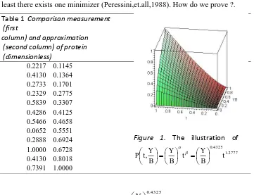
with the error 0.9008 %. This result is considerable good. Since the data

are not too large, we may make a list of each value of the approximation

compared to the observation (shown in Table 1) and it is depicted in

Figure 1. Now,one may proceed the optimization goal ,i.e maxP subject

to the constraints ₁( , , ) 0

     

B Y t B Y

g andg₂(Y,B,t) t > 0.

Unfortunately, the standard procedure in literature for an optimization is

MATLAB is usually proposed a minimization solver. Therefore one may

set up the optimization model as :

     

   

       

       

. 0 )

, , ( ~ , 0 )

, , ( ~

to subject )

( min )

(

2 1

2777 . 1 4325 . 0

t t B Y g B

Y t

B Y g

t B Y x

f P



MATLAB provides fmincon.m function to solve this minimization problem.

Up to this step, the program can not give a reasonable solution. One reason is

due to the property of the objective function which is not coercive

(i.e 



 ( )

lim f x x



) If the objective function is coercive then it is guaranteed at

[image:6.468.117.355.124.176.2]

least there exists one minimizer (Peressini,et.all,1988). How do we prove ?.

Table 1 _{Comparisan measurement}

(first

column) and approximation (second column) of protein (dimensionless)

0.2217 0.1145 0.4130 0.1364 0.2733 0.1701 0.2329 0.2775 0.5839 0.3307 0.4286 0.4125 0.5466 0.4658 0.0652 0.5551 0.2888 0.6924 1.0000 0.6728 0.4130 0.8018 0.7391 1.0000

Figure 1. The illustration of 2777 . 1 4325 . 0

, t

B Y t B Y B Y t

P 

                 

  

Note that 1.2777

4325 . 0 ,

,lim )

(

lim t

B Y x

f

t B Y

x 

      _

 



which tends to minus

[image:6.468.62.423.276.553.2]

7

objective function since it has been obtained from the previous optimization

process. Thank to Peressini(et all,1988), that it offers the idea to perturb the

objective function. More specifically, for each  0, define

2 )

( )

(x f x x

f      . (7)

Unfortunately, we need also property that f(x) is convex

(Peressini,et.all,1988,page 52) i.e

) ( ) ( ) ( )

(x f x y x f y

f         , y,x in a convex set subset of Rn. (8) Let us try to study this condition for all values in the given domain and we

write into more general form,i.e f(x)= 

 t B Y      

 . As a consecuence, one

needs to compute ( ) 1 ( 1) 1 1 .

T

t B Y t Y YB t

B Y x

f _

  

  

      



  _    _     

Using the values, in the given domain we obtain that the

condition (8) is satisfied for yx. This is shown on Figure 2. Thus, the

property (8) is satisfied and hence the function f(x)= 

 t B Y      

 is

convex. Clearly, the x 2is a quadratic function which is known to be convex. Therefore the perturbed function defined Eq.( 7) is convex. We

are done to show that f(x)is convex. The proof that f(x) is coercive

is not shown here for simplicity, which is mentioned into detail in

Peressini (page 229). The optimization problem becomes

     

   

       

        

. 0 )

, , ( ~ , 0 )

, , ( ~

to subject )

( min )

(

2 1

2

t t B Y g B

Y t

B Y g

x t

B Y x

f P



  _{ }

[image:8.468.66.407.71.239.2]

Figure 2.

Illustration of f(x)f(x)(yx) f(y)obtained by each value of

y>xfrom the given domain.

Penalty Method with a noncoercive objective function f(x)

We need to construct the Lagrangian L(x,)for Pas follows

) ( ~ )

( ) , (

1

x g x

f x

L

m i

i i

 





_



 

 

 _{, m = the number of constraints.}

This Lagrangian becomes an unconstraint objective function with additional 2

unknown parameters.We can use the function fminunc.m in MATLAB by

defining the Lagrangian function as the objective function. We have tried 5 sets

of initial guesses and the observation shows unreasonable answers. Analytic

observation will explain why the function fminunc.m and fmincon.m do not

give unique solutions.

One needs to construct L(x,)0 analytically and solve it by solver of nonlinear system equations. We have

0 2

) , ( : ) ,

( 1

1 1

1    

 

 _{g x Y}  _B _{t Y B}

Y x L

  



   

  _{ }

; (9a)

 

0 2

) , ( : ) ,

( 2

1 )

1 (

2    

 

 _{g x Y B}  _{t B YB}

B x L

  



   

  _{ }

; (9b)

, 0 2

) , ( ) , (

2 1

3    

 

   _{g x  Y}_B_t _{t }

t x

L   

(9c)

0 )

, ( ) , (

4 1

         

 

B Y x

g x

L



 

   _{ }

9

. 0 )

, ( ) , (

5 2

   

 

t x

g x

L



 

   _{ }

(9e)

We write the system as g(x)



g₁ g₂ g₃ g₄ g₅



T 0. One obtains directly from Eq.(9e) and Eq.(9d) that t*=0; Y* 0 respectively. Substitute these result to Eq,(9c), one yields *2 0. As a result, 0

* 1   to satisfy Eq.(9b). On the other hand B* 0since it will make Eq. (9b) is undefined if B* 0. Therefore B* 0 and it is free variable. Thus the

system has infinitely many solutions in the form

) 0 , 0 , 0 , , 0 ( ) , , , ,

( *2

* 1 * * *

a t

B

Y    with a 0. Moreover this conclusion is

practically useless. However this explains us that the Newton method

will not converge if this method is used blindly. By forcing g(x) tends

to zero (as shown in the Figure) , the solution x* is not a real vector after 747 iterations though the method works well by showing that g(x) tends to zero

as depicted by Figure 3. Thus the Newton method fails which agrees with

[image:9.468.109.375.427.547.2]

analytic result.

Conclusion

This paper has presented an example of using the optimization solver

provided by MATLAB. The used data is considered as a smooth function of 3

variables. After the parameters are obtained the optimization is employed to

obtain the minimizer of the noncoercive objective function.

The minimizer is obtained by solving the nonlinear system of the

Lagrangian function which is constructed as a perturbed objective function. The

optimizer can not be considered as the best solution since the Hessian is not

positive definite. One may avoid the computation of gradient by using ant

colony algorithm, particle swarm algorithm (Rao,2009).

Aknowledgement

The author gratefully acknowledge to Yohanes Martono for supporting his data to this numerical work with MATLAB .

References

Buong,N and Dung. D, (2009).Regularization for a Common Solution of a System of Nonlinear Ill-Posed Equations, Int. Journal of Math. Analysis,3(34), 1693-1699.

Grosan, C and Abraham, A,(2008). Multiple Solutions for a System of Nonlinear Equations, International Journal of Innovative Computing, Information and Cotrol, x( x), ISSN 1349-4198.

Jones, T.A, (2006). MATLAB functions to analyze directional (azimuthal) data-I:Single-sample inference, Computers & Geosciences

32 (2006) 166-175.

Peressini, A.L, Sullivan, F.E, Uhl,J, (1988). The Mathematics of Nonlinear Programming, Springer Verlag, New York, Inc.

Rao, S.S. (2009). Engineering Optimization, Theory and Practice, John Wiley & Sons, Inc., Hoboken, New Jersey.

Sander C, and Scheider,R, (1991). Database of homology-derived protein structures and the structural meaning of sequence alignment, Protein, 9(1),56-68.