Gender Wage Disparities among the
Highly Educated
Dan A. Black
Amelia M. Haviland
Seth G. Sanders
Lowell J. Taylor
a b s t r a c t
We examine gender wage disparities for four groups of college-educated women—black, Hispanic, Asian, and non-Hispanic white—using the National Survey of College Graduates. Raw log wage gaps, relative to non-Hispanic white male counterparts, generally exceed -0.30. Estimated gaps decline to between -0.08 and -0.19 in nonparametric analyses that (1) restrict attention to individuals who speak English at home and (2) match individuals on age, highest degree, and major. Among women with work experience comparable to men’s, these estimated gaps are smaller yet—between -0.004 and -0.13. Importantly, we find that inferences from familiar regression-based decompositions can be quite misleading.
I. Introduction
In U.S. labor markets women earn substantially less than men. Hun-dreds of studies investigate this phenomenon, seeking to infer the extent to which the gender wage gap is the consequence of disparate treatment by employers. The statis-tical exercise is one of comparison; at issue is the difference between the wages women receive and those earned by males who are otherwisecomparablein terms
Dan A. Black is a professor at the Harris School at the University of Chicago and a senior fellow at NORC; Amelia M. Haviland is a statistician at RAND Corporation; Seth G. Sanders is a professor of economics at Duke University; and Lowell J. Taylor is a professor at the Heinz School at Carnegie Mellon University. The authors gratefully acknowledge financial support from the NICHD, and thank seminar participants at the University of Chicago, University College London, London School of Economics, Florida Atlantic University, University of Michigan, Notre Dame, Texas A&M University, Yale University, and the annual meetings of the Population Association of America. The data used in this article can be obtained beginning January 2009 through December 2012 from Amelia M. Haviland, RAND Corporation, 201 North Craig Street, Pittsburgh, PA 15213,
haviland@rand.org.
½Submitted July 2006; accepted July 2007
ISSN 022-166X E-ISSN 1548-8004Ó2008 by the Board of Regents of the University of Wisconsin System
of relevant characteristics (that is, men with similar levels of human capital). The standard means of drawing such comparisons, used in nearly every paper on the topic, is linear regression; the idea is to ‘‘control’’ for factors that reflect differences in preferences and human capital between men and women. Gender wage differen-tials that remain after such adjustments are often taken as evidence of labor market discrimination.1
Research using large representative data sets, such as the Current Population Sur-vey (CPS) or the U.S. Census, shows that the human capital model explains very lit-tle of the observed wage gaps between men and women. But large data sets such as the CPS and Census typically lack sufficient detail on relevant human capital varia-bles; they typically have no data on years of work experience and have only rudimen-tary information on educational attainment. In the absence of adequate measures of premarket human capital, researchers can use industry and occupation indicators as proxies for market skills, but this practice complicates interpretation of the estimated gender wage gap if industry and occupation assignments are themselves the conse-quence of disparate labor market treatment.
An alternative research approach is to rely on smaller specialized data sets that have greater labor market detail and carefully collected information on education. The relatively small size of these data sets can make inference about the gender wage gap problematic, particularly when the research focuses on a subset of the popula-tion, college-educated individuals. To draw inferences of reasonable precision researchers typically adopt parametric approaches—relying on assumptions that have been called into question in the recent literature.2
As we have noted, a large literature studies the gender wage gap, and studies have adopted widely different regression specifications, and made use of different data sets covering different time periods (while generally following one of the two research approaches noted above). Although there is, not surprisingly, considerable variability in inferences concerning gender wage gaps, there are also some broadly accepted generalizations. It appears that the wages of women were about 35 to 40 percent lower than the wages of men from the 1920s through the mid-1980s, and then started to converge (Smith and Ward 1985; and Mulligan and Rubinstein 2005, for more re-cent trends). Several studies find that the raw gender wage gap was between 25 and 30 percent by the mid-1990s. The portion of the gender wage gap explained by prel-abor market skills and occupational choice varies across studies. As one might ex-pect, the more detailed the premarket skills or occupational choices reported in the data, the larger the share of the gender wage gap that is ‘‘explained.’’3In most 1. As discussed below, even if researchers can properly ‘‘control’’ for observed differences in human cap-ital investment, interpretation can be problematic, as such differences may themselves reflect anticipated or prelabor market discrimination. Models that control for human capital investment can be more narrowly interpreted as isolating disparate treatment experiencedinthe labor market from differencespriorto enter-ing the labor market without assignenter-ing cause to the observed premarket differences. Understandenter-ing whether employers pay comparable workers comparable wages—the isolated effect—is still of obvious importance for understanding gender wage gaps.
2. For example, Heckman, Lochner, and Todd (2006) express concerns about regression-based models of wage determination.
3. For example, Kidd and Shannon (1996) show that considering the sorting of men and women into 36 rather than nine occupations increases the share of the wage gap explained by occupational sorting from 12 percent to 27 percent.
studies, at least one-third of the gender wage gap remains even after carefully con-ditioning on prelabor market skill differences andon factors—such as occupation, labor market experience, and tenure with the employer—that could themselves be affected by discrimination experienced while in the labor market. Even if one accepts as a working assumption that occupational sorting is not the result of discrimination, there is evidence of gender wage disparities—disparities that occur within occupa-tions and industries.
The literature has led many people to believe that the evidence of market discrim-ination against majority women is stronger than the evidence of market discrimina-tion against minority men. The logic is compelling. When researchers compare economic outcomes of black or Hispanic men with their non-Hispanic white counter-parts, non-Hispanic white men are seen to have considerable prelabor market advan-tages. For instance, these men not only have more schooling than black and Hispanic men, on average, but also have access to better schools. There are, in short, substan-tial racial and ethnic differences in premarket opportunities to build human capital. In contrast, non-Hispanic white men and women are born to the same parents, attend the same schools, and in recent years they have similar rates of high school and col-lege completion. While there is mounting evidence that prelabor market differences explain almost the entire black-white wage gap for men, these same factors explain very little of the white non-Hispanic gender wage gap.4
Against this backdrop, we conduct here an analysis that makes several contribu-tions to the gender wage gap literature—contribucontribu-tions that ultimately derive from our use of an unusually valuable data source, the National Survey of College Grad-uates (NSCG).5In 1993, the NSCG resurveyed 214,643 individuals who indicated on their 1990 Census form that they had completed a bachelor’s degree or an advanced degree. The size and detail of the NSCG allow us to address three issues for college-educated men and women.
First, the large sample size of the NSCG gives us license to explore an issue that is almost entirely neglected in the literature on the gender wage gap—the importance of restrictive parametric assumptions that underlie regression-based analyses.6Our use of nonparametric matching forces us to confront the ‘‘support’’ on which our inferences are drawn—an issue easily obscured in parametric work. As we note above, the central idea of all wage gap studies is to contrast the wages earned by women with those ofcomparablemen. This issue of ‘‘support,’’ in a nutshell, is that owing to gender-related premarket sorting there are many women for whom there are no convincing male comparables. For example, there are many older women in the 4. Neal and Johnson (1996) report that black and white men in the National Longitudinal Survey of Youth, 1979 (NLSY79) with the same level of prelabor market skills (as measured by the Armed Forces Qualifying Test score (AFQT)) have quite similar earnings. In contrast, Altonji and Blank (1999) find that in 1994 vir-tually the entire gender wage gap remains even after accounting for AFQT scores.
5. Very little work on gender has been done using these data. In one exception, Graham and Smith (2005) report on gender differences in employment and earnings in science and engineering occupations. 6. Nonparametric methods have recently been used in some work on wage determination, though rarely in the study of gender wage gaps. Using a nonparametric kernel smoothing method applicable to mixed con-tinuous and categorical data, Racine and Green (2004) test and reject the traditional parametric model. Sim-ilarly, Heckman, Lochner, and Todd (2006) test and reject the functional form of the Mincer earnings regression for the last 30 years of Census data. Nopo (Forthcoming) uses nonparametric analysis in his study of gender wage gaps in Peru.
United States who earned a bachelor’s degree in nursing, but few, if any, similarly aged men with this same education. When we conduct analyses that match on both premarket characteristics (age and educational characteristics)andyears of experi-ence, the situation becomes even more difficult. Many college-educated women have sustained periods when they are not in the labor force, but few men do (and those men who do have limited labor market attachment may in any event be poor com-parables). In our nonparametric analysis, we cannot sweep these issues under the rug by making functional form assumptions.7
Second, we are able to explore the role of the substantial existing gender differen-ces in training at the bachelor’s level and above. Male-dominated majors, such as chemical engineering, may generally have higher returns than such female-domi-nated majors as elementary education, and these differences in prelabor market choices are a potentially crucial part of the story in understanding the gender wage gap among the well educated.8The role of college major on earnings and the impact on gender wage gaps in the United States has been documented in several studies, including Altonji (1993), Brown and Corcoran (1997), Eide (1994), Graham and Smith (2005), Grogger and Eide (1995), Joy (2003), Loury (1997), McDonald and Thornton (2007), Paglin and Rufolo (1990), Turner and Bowen (1999), and Weinberger (1998, 1999). While all of these studies report that college major is associated with some portion of the wage gap, they differ in the size attributed to college major. In our reading, much of this difference is the result of the extent of aggregation of the col-lege majors; the finer the detail in the measurement of colcol-lege major, the greater the fraction of the wage gap that is explained by the major. Indeed, Machin, and Puhani (2003) demonstrate similarly that college major is important to understanding wage gaps in the United Kingdom and Germany, and further indicate that use of more detailed major categories allows one to explain a higher portion of the gender wage gap. Our data have far greater detail on college major than previous research, and we are in ad-dition able to explore the extent to which parametric methods influence inferences drawn about the role of major on wages.
Third, the large sample size of the NSCG allows us to conduct our analyses for four distinct racial and ethnic groups of women: non-Hispanic white, Hispanic, black, and Asian. There is, of course, inherent interest in the role of race and ethnic-ity in labor market outcomes for women, but there is an additional conceptual mo-tivation for studying gender wage differences by ethnicity and race.9 As we show below, among college-educated women there are substantial differences by race and ethnicity in the distributions of college major. For example, Asian women select college majors that are more similar to men’s majors than do other women (that is, in comparison to other female groups, a disproportionately high fraction of Asian women study engineering and computer science). An examination of wage patterns for Asian women is thus potentially helpful in drawing inferences about the likely
7. This theme is nicely developed in the analysis of black-white differences in asset ownership by Barsky, Bound, Charles, and Lupton (2002).
8. There is a substantial literature on the topic of lower wages in female dominated occupations, for exam-ple see Bergman (1974).
9. In their examination of known work on gender and race in the labor market, Altonji and Blank (1999) suggest that the role of race and ethnicity among women in the labor market is an important understudied area.
effect on the gender wage gap of a more general shift by women toward male-dom-inated college majors.
Quite clearly, the primary focus of our paper is the vital role of early human capital investments for understanding subsequent earnings of men and women. Our paper has considerably less to say about two other issues that have received considerable attention: selection into the labor force and issues of household labor supply.10Based on the theory of comparative advantage for home production, we might expect women to invest in different forms of human capital and to have lower levels of labor market participation over their life cycle.11As Becker (1985) cautions, it is likely that if women make observably different investments in their careers than men— choosing less lucrative majors or withdrawing more frequently from the labor force—they may also make unobservable decisions that will lower their wages rel-ative to men who are otherwise observationally equivalent. Thus, gender wage differ-ences that occur even among men and women with similar levels of observed human capital can reflect unobserved differences in underlying market productivity of men and women. In analyses presented near the end of the paper we do undertake some explorations of the role of labor market attachment for the gender wage gap, but as will be clear we have a limited contribution to make concerning this important issue. Our paper proceeds as follows: In Section II we discuss our data, the NSCG, and the unique advantages it has for studying the gender wage gap among the highly ed-ucated. In Section III, we briefly outline the traditional regression-based approaches to estimating the gender wage gap and, as a means of establishing a baseline for com-parison, conduct such an analysis using the NSCG. Section IV presents our nonpara-metric matching method and discusses subtle issues in constructing standard errors for these estimates. We present key findings in Section V and provide concluding remarks in Section VI.
We briefly preview our results. Using nonparametric matching, we compare the log wage of women—separately for non-Hispanic white, black, Hispanic, and Asian women—with non-Hispanic white men. Raw log wage gaps are substantial, between -0.26 and -0.34 across racial/ethnic groups. Our baseline comparison matches women to male counterparts on premarket characteristics only: exact highest degree, major, and age. Consistent with previous literature, we find that very little of the gen-der earnings gap stems from gengen-der differences in the highest degree attained. Col-lege major, in contrast, is important for subsequent earnings. Among women who speak English at home between 44 and 73 percent of the gender wage disparity is accounted for by highest degree, major, and age. By further restricting attention to women who have ‘‘high labor force attachment’’ (work experience that is similar to male comparables) we explain all but -0.13 to -0.004 log points of the gender wage gap. Our nonparametric approach differs from the familiar Blinder-Oaxaca
10. See Mulligan and Rubinstein (2005) for a nice statement of the issues concerning selection and human capital investment, and references to further literature.
regression decompositions, so for the sake of comparison we conduct the parametric analyses as well. We find that in our context inferences drawn from these latter decompositions can be quite misleading.
II. Data and Distributions of Highest Degree and Major
by Gender, Race, and Ethnicity
The data set used in this research is the 1993 National Survey of College Graduates (NSCG). The NSCG stems from an initiative of the National Sci-ence Foundation (NSF) to compile information on scientists and engineers. The NSF and the Census Bureau drew a stratified sample of 214,643 individuals based on the 1990 Decennial Census Long Form, with the sample limited to those reporting both a baccalaureate degree (at least) and age no greater than 72 as of April 1, 1990. The Census Bureau first contacted individuals by mail, then, if necessary, followed up with a telephone or in-person interview. In the collection of these data, a great deal of attention was paid to the accuracy of the education responses. Detailed informa-tion was gathered about the majors of the respondents for up to three degrees. In ad-dition, the NSCG included better measures for labor market experience than is provided in the Census (in particular, the number of years of full-time work). An additional important feature of the NSCG is that a number of the respondents’ 1990 Long Form responses were made available for analysis in the NSCG.
From those selected to be in the sample based on their 1990 Census data, it was found by 1993 that a few had emigrated from the United States (2,132), died (2,407), or were institutionalized (159) and were hence out of the survey’s scope. Some were found to have misreported their age and were older than 75 years old (211). Surpris-ingly, 14,319 respondents had no four-year college degree despite reporting, or being imputed to, a four-year degree on the 1990 Census. Another 46,487 declined to participate fully in the NSCG and information crucial to the analysis was missing (that is, they failed to provide information about their last degree and field of study). Once the out-of-scope groups are excluded, there is a (weighted) response rate of 80 percent, or a sample of 148,928 respondents. In this paper we examine women and non-Hispanic white men only (which reduces the number of observations by 19,046) and because of the small sample size we choose to omit Native American women from the analysis (which reduces the sample by 630), giving 129,252 respondents who are non-Hispanic white men or women, or black, Hispanic, or Asian women.
Because the sampling frame of the NSCG is the 1990 Census Long Form, anyone not having a degree by 1990 would not be included in the sample. As a result, we restrict our sample to individuals who are at least 25 years of age (in 1990) to insure that most individuals would have had the opportunity to complete their undergradu-ate education. Similarly, to avoid complications that might arise with differential re-tirement ages, we restrict our sample to workers 60 years old and under. These age restrictions reduce the number of observations by 18,033. A small number of sub-jects are excluded due to item nonresponse (imputed answers) to gender, race, age, or ethnicity questions, reducing the number of observations by 3,032. A much
larger proportion is excluded by item nonresponse related to the calculation of wages: We omit those who had imputed or zero wage incomes (16,286) and those who had imputed weeks worked or usual hours worked (9,079). Workers who reported self-employment income in addition to wage income were not included in our sample because there is no way of determining whether the hours and weeks worked refer only to the wage-earning job or to the self-employment job also, which would bias the calculated hourly wage (this restriction reduces the number of ob-servations by 8,060). Another 149 respondents reported no major for their highest degree, and we dropped these respondents from most of our analyses. These exclu-sions leave us with a sample of 74,613 respondents. Because the data oversampled certain populations, in what follows we weight the data to reflect the sampling weights.
The NSCG provides detailed data on each respondent’s education, including iden-tification of more than 140 different majors. Table 1 provides evidence on the sys-tematic heterogeneity in educational outcomes among individuals with at least a four-year college degree. In comparison to the benchmark majority group—non-Hispanic white men—women in each ethnic and racial group are less likely to pursue graduate education, especially the professional degree and PhD. There are also very large differences in the choice of college major at the undergraduate level.12Women are generally underrepresented in the highest-paying majors, especially engineering, and overrepresented in such low-paying majors as education, the humanities, and the fine arts; 26 percent of non-Hispanic white men major in the five lowest paying majors (education, humanities, professional degrees, fine arts, and agricultural scien-ces), as compared with approximately 50 percent of white, black, and Hispanic women and 22 percent of Asian women. Among these racial and ethnic groups of women, Asian women have a distribution of majors most like men. The index of dis-similarity, reported in the last line of Panel B, estimates the percentage of women in each group that would need to be strategically reallocated to another major for the distribution of majors to match that of white men.13 For white, black, Hispanic, and Asian women respectively, 45, 44, 42, and 36 percent would need to change ma-jor to match the mama-jor distribution for non-Hispanic white men. These patterns are seen again in Panel C, which shows the mean fraction female within undergraduate major for each group.
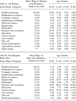
Panel A of Table 2 indicates that the distribution of undergraduate majors for women has changed markedly over recent cohorts. A particularly notable change is in the education major; 38 percent of the women in the 51–60 age cohort majored in education, compared with 15 percent for the 25–30 cohort. In contrast, there has been a large increase in business and economics majors, from 6 percent for the 51–60 cohort to 24 percent for the 25–30 cohort. Panel B provides corresponding statistics for men. Results in Tables 1 and 2 suggest that research using ‘‘years of education’’ as the lone human capital variable misses a major source of the gender-related dif-ferential in human capital, and indicate, furthermore, that the importance of this omission varies considerably by cohort.
12. In Panel B of Table 1 we aggregate our major categories.
Table 1
Distributions of Highest Degrees and Bachelor’s Major for Women and Men
Panel A: Highest degree
White Black Hispanic Asian
F M F M F M F M
Bachelor’s 70.20 63.34 67.71 68.28 69.28 65.44 72.32 54.24
Master’s 24.66 22.89 27.97 22.57 23.68 20.90 19.59 27.13
Professional degree 3.28 9.00 2.70 5.69 4.34 9.58 5.81 10.02
PhD 1.87 4.76 1.62 3.46 2.70 4.08 2.29 8.62
N 36,256 56,524 6,514 4,887 3,250 4,103 5,422 7,633
Panel B: Bachelor’s Major
Mean Wage of Men with Bachelor’s
Degrees by Field White Men
White Women
Black Women
Hispanic Women
Asian Women
Engineering $25.43 12.72% 1.04% 0.70% 1.85% 3.77%
Mathematical sciences 22.18 2.53 1.74 1.53 1.20 2.62
Business and economics 21.68 28.10 12.08 16.75 16.06 21.24
Physical sciences 19.96 4.57 1.25 0.91 1.36 4.08
Social sciences 19.69 13.91 13.90 16.56 15.45 9.96
Engineering technology 19.29 1.88 0.10 0.17 0.29 0.21
Health professions 19.24 2.61 10.47 8.92 9.00 16.64
Black,
Haviland,
Sanders
and
T
aylor
Computer sciences 18.76 1.75 0.95 1.25 1.32 2.96
Life sciences 17.58 4.94 3.93 3.85 4.19 6.76
Education 17.22 8.10 27.83 29.02 23.58 10.44
Professional degrees 17.16 5.33 9.01 11.15 8.52 4.86
Humanities 17.14 6.76 10.41 5.88 11.99 9.89
Agricultural sciences 16.46 2.58 0.83 0.39 1.06 1.29
Fine arts 16.22 3.30 6.02 2.46 3.79 4.54
Major not elsewhere classified — 0.91 0.43 0.48 0.36 0.73
Dissimilarity index 0.00% 45.40% 43.55% 41.98% 35.93%
Panel C: Mean Fraction
Female within Undergraduate Major
White Black Hispanic Asian
Men 33.89% 39.15% 35.11% 26.45%
Women 61.44% 59.84% 57.60% 51.99%
Notes: The data are weighted to account for sample stratification. In Panel B, men’s mean wage of bachelor’s degree is estimated using only men whose highest degree completed is a BA, while the percentage of each group selecting each undergraduate college major includes those with higher degrees. The 144 majors in the NSCG are aggregated in Panel B, but the full set of majors is used to calculate the dissimilarity index in Panel B and all results in Panel C. Source: AuthorsÕcalculation, NSCG.
638
The
Journal
of
Human
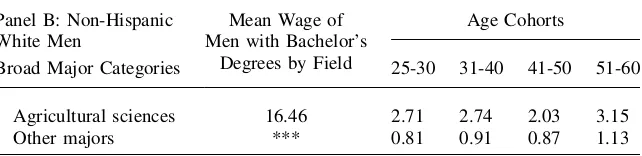
Table 2
Distribution of Undergraduate Majors for Four Cohorts of Women and Non-Hispanic White Men
Panel A: All Women
Mean Wage of Women with Bachelor’s Degrees by Field
Age Cohorts
Broad Major Categories 25-30 31-40 41-50 51-60
Health professions $16.84 10.55 11.92 9.25 9.88 Mathematical sciences 16.30 1.37 1.75 2.18 1.58
Computer sciences 15.83 2.66 0.85 0.36 0.08
Engineering technology 15.45 0.25 0.12 0.02 0.03
Physical sciences 14.87 1.45 1.31 1.24 1.59
Engineering 14.47 2.81 0.91 0.39 0.28
Humanities 14.33 6.79 9.13 13.75 11.99
Business and economics 13.91 23.93 11.57 7.56 6.27
Education 13.56 14.81 25.93 34.62 38.27
Social sciences 13.42 12.50 14.70 14.93 12.39
Life sciences 13.09 4.63 4.72 3.18 2.80
Fine arts 12.67 5.07 6.23 5.47 5.66
Professional degrees 12.48 11.10 9.49 6.44 8.42 Agricultural sciences 11.08 1.51 0.98 0.22 0.29
Other majors *** 0.58 0.40 0.38 0.48
Panel B: Non-Hispanic White Men
Mean Wage of Men with Bachelor’s
Degrees by Field
Age Cohorts
Broad Major Categories 25-30 31-40 41-50 51-60
Health professions $19.24 1.74 2.95 2.37 3.42
Mathematical sciences 22.18 1.76 2.06 3.56 2.50
Computer sciences 18.76 4.48 1.85 0.67 0.20
Engineering technology 19.29 2.75 1.82 1.58 1.51
Physical sciences 19.96 3.92 4.23 4.70 5.82
Engineering 25.43 14.85 10.75 11.43 16.59
Humanities 17.14 4.80 6.50 7.75 7.85
Business and economics 21.68 32.69 26.87 27.04 26.98
Education 17.22 3.90 7.77 9.89 10.60
Social sciences 19.69 10.21 15.16 16.32 11.39
Life sciences 17.58 4.39 6.12 4.77 3.50
Fine arts 16.22 3.66 3.79 2.97 2.50
Professional degrees 17.16 7.32 6.50 4.05 2.86
III. Traditional Parametric Measures of Wage Gaps
The primary focus of our paper is a nonparametric investigation of wage differentials that exploits the detailed educational information we have just described. Before turning to that analysis, though, we take a brief digression to out-line the more usual parametric approaches.
A very large number of papers use linear regression to study the wage gap be-tween men and women, typically adopting one of two approaches—a ‘‘pooled re-gression’’ or ‘‘group-specific rere-gression’’ model. In the first of these approaches, the logarithm of individual wage is regressed on control variables thought to reflect individual-level differences in productivity or preferences and an indicator variable equal to one if the respondent is a woman. The residual earnings differences be-tween groups, as reflected in the coefficient on this dummy variable, can be taken as evidence of disparate labor market treatment. A typical exercise of this sort is reported by Altonji and Blank (1999) in their review piece on gender wage gaps. They specify
yi¼am ++j2ff;b;hgajdi+Xi#b+ei;
ð1Þ
wheremrefers to men, andf, b, andhrefer to female, black and Hispanic respec-tively, and yi is the natural logarithm of wages.14This specification is referred to
as the ‘‘pooled regression’’ model as the parameters on covariates, the bÕs in the model, are estimated from the pooled data for men and women.
As we note above, there is debate about what factors to include among covariates
X. Prelabor market skills are generally included (that is, the level of schooling com-pleted). Age or potential labor market experience (as measured by age – years of Table 2 (continued)
Panel B: Non-Hispanic White Men
Mean Wage of Men with Bachelor’s
Degrees by Field
Age Cohorts
Broad Major Categories 25-30 31-40 41-50 51-60
Agricultural sciences 16.46 2.71 2.74 2.03 3.15
Other majors *** 0.81 0.91 0.87 1.13
Notes: The data are weighted to account for sample stratification. Mean wage of bachelor’s degree is es-timated using only women or men whose highest degree completed is a BA, while the percentage of each group selecting each college major includes those with higher degrees. The 144 majors in the NSCG are aggregated into the broad categories shown in these tables. Source: AuthorsÕcalculation, NSCG.
14. If gaps between non-Hispanic white men and specific race or ethnic groups of women are of interest, indicator variables for each group can be included. In Equation 1, the difference between white women and white men is measured byaf, between black women and white men byaf+ab, and between Hispanic women and white men byaf+ah.
education – 6) is also usually included. There is less agreement on whether to include the respondent’s occupation, industry, and sector of employment. The consensus opinion expressed by Blau and Ferber (1987) is that ‘‘specifications which exclude occupation (and other similar variables) yield upper-bound estimates of discrimina-tion and those which include such variables yield a lower bound estimate.’’
In any event, results from Altonji and Blank (1999), reported in the first line of Panel A in our Table 3, are typical. Using data from the March 1996 Current Pop-ulation Survey, Altonji and Blank estimate the wage gap between adult women and men using Equation 1. The estimate ofaf in the first column, 20.279, is for
a specification that has no covariates other than race and ethnicity. From the second column we notice that this estimate is little changed when the researchers also in-clude education, potential experience (entered as a quadratic) and region controls. When occupation, industry, and job characteristics are included (in Column 3), though, the estimated log wage gap falls to20.221. Using Blau and Ferber’s logic
one might infer that gender discrimination accounts for large wage losses—between approximately 22 and 28 log points—and that market as well as premarket differen-ces account for rather little of the unadjusted gap.
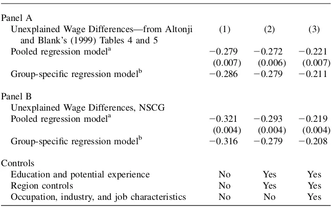
Table 3
Estimated Gender Wage Gaps using Regression-Based Specifications
Panel A
Unexplained Wage Differences—from Altonji and Blank’s (1999) Tables 4 and 5
(1) (2) (3)
Pooled regression modela 20.279 20.272 20.221 (0.007) (0.006) (0.007) Group-specific regression modelb 20.286 20.279 20.211
Panel B
Unexplained Wage Differences, NSCG
Pooled regression modela 20.321 20.293 20.219
(0.004) (0.004) (0.004) Group-specific regression modelb 20.316 20.279 20.208
Controls
Education and potential experience No Yes Yes
Region controls No Yes Yes
Occupation, industry, and job characteristics No No Yes Notes: Standard errors for group specific regression models from Altonji and Blank (1999) were not pro-vided nor do we present standard errors for the group specific estimates calculated here. The sample size for all pooled regressions in Panel B is 82,980. The sample does not include those with missing values on any controls or those whose industry was military. Sample sizes for the group specific regres-sions in Panel B are 49,661 for men and 33,319 for women. The data are weighted to account for sample stratification.
a. The coefficient on the female dummy variable is reported; dummy variables for black, Asian and His-panic are included in the model.
b. The amount of the total wage gap due to differences in group specific coefficients is reported.
An assumption implicit in the ‘‘pooled regression’’ approach is that the returns to covariates are equal for men and women. The approach taken in the alternative ‘‘group-specific’’ model is to run separate wage regressions for women and men:
yi¼Xi#bj+ei;
ð2Þ
wherej2 fm;wg, and where covariates include race/ethnicity indicator variables as in Equation 1. Having estimated Equation 2, the tradition is to decompose wage dif-ferentials between men and women into ‘‘explained’’ and ‘‘unexplained’’ compo-nents. By differencing Equation 2 across groups and taking the expected value, the Blinder-Oaxaca decomposition is:
Eðym2yfÞ ¼X#fðb^m2b^fÞ+ðX#m2X#fÞb^m;
ð3Þ
whereX#jis the mean level of earnings-related characteristics for groupj.
The term X#m2X#f
b^m is the portion of the log wage differential that is ‘‘explained’’ by the difference in the average level of earnings-related characteristics of men and women (evaluated at theb#sof men). The remaining termsX#fðb^m2b^fÞ
represent the portion of the difference in average wages due to differences in the es-timated coefficients. This is labeled the ‘‘unexplained’’ portion of the wage gap, which can be taken in principle to be the ‘‘share due to discrimination.’’
The second row of Panel A in Table 3 reports the ‘‘unexplained’’ log wage gaps that Altonji and Blank (1999) find using the group-specific regression approach. In this example the inferences one draws are the same using either of these parametric approaches: The gender log wage gap among adults in the United States in 1995 is found to be approximately 20.28 when one compares men and women with the
same education, potential experience, and region, and approximately 20.21 when one matches also on industry and occupation.
In Panel B of Table 3, we estimate the same specifications as Altonji and Blank but with the 1993 NSCG data.15The time frames are reasonably close (our wage data are taken from 1990 Census reports and are thus from 1989, while the CPS data used by Altonji and Blank are from 1995), but our analysis focuses exclusively on individuals who report having a college education. Results are strikingly similar for the two sam-ples: among the well educated, the log wage disparity is approximately20.28 in an exercise that controls for education, potential experience, and region, and approxi-mately20.21 when controls also include industry and occupation. Consistent with
previous work, we would estimate that only a third of the unadjusted gap is associ-ated with differences in premarket and market covariates.
In sum, using traditional methods we would infer that the gender wage disparity is approximately the same for well-educated women as for the workforce generally, and that this disparity is quite large. With these findings in mind we now turn to the focus of our paper: understanding the extent to which these latter inferences depend on the
15. In particular, the specification we use is a quadratic in potential experience with dummy variables to account for: race/ethnicity (black, Hispanic, and Asian), highest degree (more than a bachelors degree), re-gion (nine Census rere-gions), occupation (13 Census codes), industry (14 Census codes), whether a job is in the public sector, and if the person is working part-time.
strong assumptions made in regression-based approaches, and exploring the role of gender-specific variation in college majors.
IV. Nonparametric Matching Measures of the
Wage Gaps
In undertaking the empirical exercise of contrasting the wages of comparable men and women, nonparametric matching is an intuitive alternative to the use of linear regression. Let the raw gender wage gap be defined as
GðGjÞ ¼EðyjjGjÞ2EðyWMjWMÞ;
ð4Þ
where yj is the natural logarithm of wages for the jth group, WM indicates that
respondents are non-Hispanic white males,Gjindicates that respondents are members
of the female demographic groupj(non-Hispanic white, black, Hispanic, or Asian), andGðGjÞis the wage gap. LetXbe a vector of covariates (notincluding minority
sta-tus) andX¼x be any specific value for these covariates. Then the wage gap that is ‘‘unexplained’’ for respondents with fixed values of the covariatesX¼xis defined as
DðGjjX¼xÞ ¼EðyjjX¼x;GjÞ2EðyWMjX¼x;GjÞ
¼EðyjjX¼x;GjÞ2EðyWMjX¼x;WMÞ;
ð5Þ
which assumes that EðyWMjX¼x;WMÞ ¼EðyWMjX¼x;GjÞ for all groups of
women, in other words, assumes thatEðyWMjX¼x;GjÞis the missing
counterfac-tual—the expected log wage of a member of groupGjwith characteristicsxif she
were treated in the labor market as a white male with characteristicsx.
Given the detail of our data, in our analyses below we match on age, highest de-gree,andcollege major, and conduct analyses separately by race and ethnicity. Thus we might ask how much a 35-year-old Asian woman with a bachelor’s degree in bio-chemistry would earn if she were treated as a non-Hispanic white man in the labor market. Our answer comes from comparing her wage to the wages of non-Hispanic white men who are the same age, and have the same degree and major.
Once these counterfactuals are estimated for each member of a demographic group, the mean gap (conditional on covariates) is estimated by averaging over the gaps for each individual in the group of interest. In the program evaluation literature this estimator is said to be the effect of ‘‘treatment on the treated.’’ In this case ‘‘treatment’’ is demographic group membership. Restated, the estimator answers the question: What is the effect on log wage of being treated as a woman (of a par-ticular race or ethnicity) in the labor market, relative to labor market treatment as a similarly-aged and similarly-educated member of the majority group (non-Hispanic white men)? The interpretation given here hinges on an assumption that, given the covariates used in the matching, the dependent variableyWM has the same
expecta-tion regardless of group membership (Heckman, Ichimura, and Todd 1998). Of course, if the assumption is violated, and there are other relevant unobservables that differ by demographic group (given the age and education distribution), our estima-tor will include the impact of those unobservables as well.
There is a simple alternative interpretation of the matching approach that we use. One can think of our matching estimators as ‘‘altering the distribution of covariates,’’ so that the distributions of the covariates are identical between white males and our minority group members. This suggests that we can rewrite the matching estimator as a weighted least squares estimator, which in fact is easily done when the data are discrete. With some simple albeit tedious algebra, it can be shown that the matching estimator we use is mathematically equivalent to the weighted least squares estimates of the set of regressions of the form, lnðyÞ ¼bo+b1Gj+e, with separate regressions
for each racial/ethnic group of women, using the following weighting scheme: For all data that are not a match—both white males and members of the minority group— assigned weights are zero. For matched data, the minority group members are given a weight of one and white males are given a weight equal toPðXÞ=½12PðXÞ, where
PðXÞis the probability that the respondent is a member of the minority group, con-ditional on the covariates. This weight scheme ensures that the distribution of the covariates is the same between the treatment and control group in the matched data. Hence, our matching estimator uses none of the data for unmatched observations, but induces the covariates to be statistically independent of the minority group member-ship. As a result of this independence, there is no need for the researcher to specify (and risk misspecifying) the functional form of the conditional mean function. If we were using relatively small data sets, the loss of efficiency would of course be a mat-ter of grave concern. Given the size of the NSCG, however, we are comfortable accepting the efficiency loss that arises from not using a properly specified paramet-ric model in return for avoiding the risk of misspecifying the parametparamet-ric model. A. Nonparametric Decompositions
We can easily construct wage gap decompositions that parallel the regression-based decompositions outlined above—that is, find an average ‘‘explained’’ portion,GðGjÞ2 DðGjÞ, and average ‘‘unexplained’’ portion DðGjÞ. The raw gap can be written as a
weighted average overX,
GðGjÞ ¼+ X
pGjxEðyjX¼x;GjÞ2pWMxEðyjX¼x;WMÞ;
wherepGjxdenotes the proportion of members of groupGjwith characteristicX¼x. Adding and subtracting+XpGjxEðyjX¼x;WMÞgives us
GðGjÞ ¼+ X
pGjxfEðyjX¼x;GjÞ2EðyjX¼x;WMÞg
2+
X
fpWMx2pGjxgEðyjX¼x;WMÞ: ð6Þ
The first term in Equation 6,DðGjÞ;is the portion of the gap that is independent of
the distribution of covariates—that is, ‘‘unexplained’’ by the covariates. It is the sum of Equation 5 overXfor the probability distributionpGjx. The second term, the ‘‘ex-plained’’ portion of the wage gap, is due to group differences in the proportions of individuals across cells. The ‘‘explained’’ part of the wage gap is
GðGjÞ2DðGjÞ ¼+ X
fpGjx2pWMxgEðyjX¼x;WMÞ: ð7Þ
While these decompositions are clearly in the spirit of the usual regression-based decomposition, two distinctive features merit emphasis. First, our focus is on the im-pact of ‘‘treatment on the treated’’ obtained by averaging over the support of the characteristics of interest within the group of interest, not for the non-Hispanic white male distribution or a pooled distribution.16Second, our method is entirely nonpar-ametric—based on matching each woman in a particular racial/ethnic group to cor-responding non-Hispanic white males. As will be apparent shortly, in some of our analyses there are substantial proportions of women for whom we are unable to form matches with comparable men. Our approach is to draw inferences on the basis of cases for whom we can make direct comparisons, while remaining generally silent about wage disparities that might exist for women for whom we have no male com-parables. Recent work by Barsky, Bound, Charles, and Lupton (2002) highlights the perils of the alternative approach—making parametric assumptions for the purpose of matching where there is no support. In reporting our estimated wage gaps we re-port matching rates, to give readers a sense of the severity of the supre-port problem in our empirical work.
B. Standard Errors
To estimate standard errors for the results of the matching model we use a nonpara-metric bootstrap procedure. There are two advantages to using a nonparanonpara-metric boot-strap in this setting. First, it allows us to incorporate the variability of the matching cell sizes due to random sampling and nonresponse. Second, it allows us to take ad-vantage of the variance-reducing attributes of the stratified sampling design of the NSCG. In order to estimate the effect of ‘‘treatment on the treated’’ we average the differences in mean log wages over the distribution of age, highest degree, and field of study for each demographic group of interest. The weighted counts within each of the discrete cells of this distribution are themselves random variables, and the bootstrap incorporates the variance of these cell sizes into the overall variance estimate. In addition, the matching cell sizes are affected by unit and item nonre-sponse. These sources of variation are accounted for by resampling the original sam-ple, before exclusions are made due to unit or item nonresponse, or being out of scope for the survey or this analysis. Then the exclusions are applied to each resampled data set, resulting in a random effective sample size and a random match-ing cell size. This procedure is an alternative to that presented by Canty and Davison (1999), who also recommend resampling the full original sample, but then reestimate the adjusted sampling weights within each resampled data set (so that the final sam-pling weights are random variables).17As is common for large public-use data sets,
16. This distinction highlights that the difference in wage gap estimates obtained by averaging over the women’s or men’s distributions, referred to as the indeterminacy of the Blinder-Oaxacca decomposition, is simply the consequence of estimating different parameters—the effect of the ‘‘treatment on the treated’’ or the effect of ‘‘treatment on the untreated.’’
17. Canty and Davison (1999) found that incorporating the variance of these random adjusted sampling weights substantially changed their variance estimates when estimating common labor force outcomes.
we did not have the information necessary to recreate the adjustments. The alterna-tive we use leaves the individual sampling weights fixed, but the sum varies over any unit of grouping and thus the relative weight of each person in the resampled data sets varies across bootstrap samples.
Stratified sample designs are variance reducing as long as the variance within sam-pling strata is smaller than the variance in the entire sample. The variance is reduced by calculating the overall variance as the (weighted) sum of the variance within each stratum so that the between-strata variance is omitted. This variance-reduction prop-erty is incorporated into the bootstrap by resampling independently within each stra-tum to create each resampled data set. Because Shao and Tu (1995) show that this simple within-strata procedure produces variance estimates that are too small when some of the strata are small, we use a modified bootstrap method referred to as the ‘‘with-replacement bootstrap’’ in Shao and Tu (1995, p. 247). The modification con-sists of resamplingnh21 observations instead ofnhobservations from each stratum,
with replacement, where the stratum size isnhfor stratumh. The standard errors
pre-sented in this paper for the nonparametric matching estimates and Table 7 are based on 1,000 bootstrap iterations. See Haviland (2003) for a discussion with more details.
V. Empirical Findings
A. Nonparametric Matching on Premarket Factors
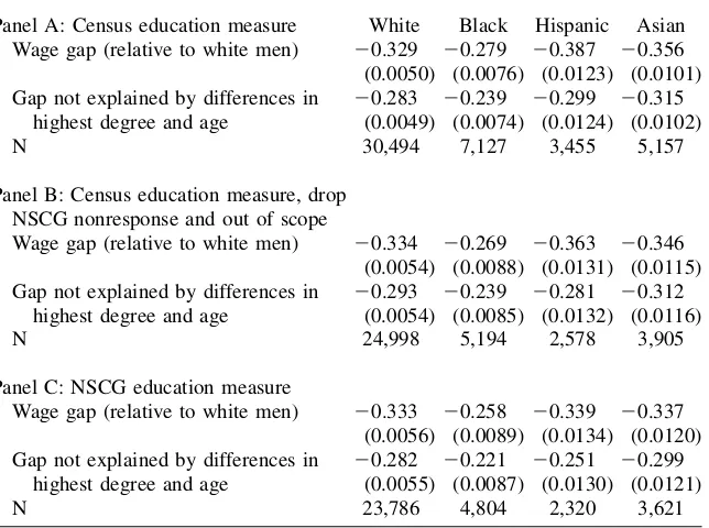
Our first nonparametric results, presented in Panel A of Table 4, are the unadjusted gender wage gaps as measured using wage and education data from the 1990 Census, which were provided by the women and non-Hispanic white men who were selected for the NSCG sample (that is, who reported having a bachelor’s degree or higher in the 1990 Census and who were selected to be in the NSCG). The unadjusted gap is calculated as the difference in the (weighted) mean log wage for the demographic group of interest and the (weighted) mean log wage for white men.18 Using the matching method described above, matching on age and highest degree, the absolute value of log wage gaps decline by a modest amount for each demographic group of women.
Before turning to our general analysis, we dispense with a potentially troublesome issue of data quality—the poor measurement of educational level among the well ed-ucated. Related work (Black, Sanders, and Taylor 2003) indicates that the misreport of higher education is substantial, and varies by gender and race in the U.S. Census. We argue in that paper that the education reports in the NSCG are likely to be much more accurate. Panel B reports the same estimation used in Panel A but with a sam-ple that drops those selected to be in the NSCG who did not fully respond or who were out of scope (for reasons other than not having at least a four-year college de-gree). The unadjusted and adjusted wage gap estimates change only slightly. Results
18. At this stage, no balancing over the different age and educational characteristic distributions is done. The estimated raw wage gaps of -0.33, -0.28, -0.39, and -0.36 for non-Hispanic white, black, Hispanic, and Asian women respectively, compare with estimates of -0.36 to -0.37 found for women generally by Brown and Corcoran (1997) using 1984 data for college-educated individuals from the Survey of Income and Pro-gram Participation.
reported in Panel C are based on the NSCG measure of highest degree; changes tween Panels B and C are due to differences in the reporting of highest degree be-tween the Census and the NSCG.19 Point estimates are slightly lower when the more accurate NSCG data are used, with the biggest changes recorded for Hispanic women, whose estimated log wage gaps drop by 0.02 to 0.03. We use NSCG educa-tion data in all subsequent analyses.
Table 5 presents our key analyses of the role of premarket factors on the wage gap. Panel A shows that a relatively modest portion of the log wage gap, 0.04 to 0.09, is explained by highest degree and age. By comparing the unexplained gaps in Panels A and B, we note that including major for non-Hispanic white, black, and Hispanic women causes the log wage gaps decrease considerably—by approximately 0.10. For these three demographic groups, age, highest degree, and major account for be-tween 45 percent and 53 percent of the gender wage gap. These same factors explain Table 4
Gender Wage Gaps—The Role of Census Measurement Error
Panel A: Census education measure White Black Hispanic Asian Wage gap (relative to white men) 20.329 20.279 20.387 20.356 (0.0050) (0.0076) (0.0123) (0.0101) Gap not explained by differences in
highest degree and age
20.283 20.239 20.299 20.315
(0.0049) (0.0074) (0.0124) (0.0102)
N 30,494 7,127 3,455 5,157
Panel B: Census education measure, drop NSCG nonresponse and out of scope
Wage gap (relative to white men) 20.334 20.269 20.363 20.346
(0.0054) (0.0088) (0.0131) (0.0115) Gap not explained by differences in
highest degree and age
20.293 20.239 20.281 20.312
(0.0054) (0.0085) (0.0132) (0.0116)
N 24,998 5,194 2,578 3,905
Panel C: NSCG education measure
Wage gap (relative to white men) 20.333 20.258 20.339 20.337
(0.0056) (0.0089) (0.0134) (0.0120) Gap not explained by differences in
highest degree and age
20.282 20.221 20.251 20.299
(0.0055) (0.0087) (0.0130) (0.0121)
N 23,786 4,804 2,320 3,621
Notes: The data are weighted to account for sample stratification. Estimates are from nonparametric regres-sions. All differentials are computed relative to white men. In Panels A and B, we match workers on their age and Census-reported highest degree. In Panel C, we match workers on their age and NSCG-reported highest degree. Bootstrapped standard errors are reported in parentheses based on 1,000 replications. Source: AuthorsÕcalculation, NSCG.
19. The sample sizes decrease in moving from Panel B to Panel C because of those people who reported (or had imputed) having at least a four-year college degree on the Census but who reported they did not when they were responding to the NSCG.
a smaller portion of the gender wage gap between Asian women and non-Hispanic white men, as Asian women’s majors are more similar to white men’s majors than are those of other women.20
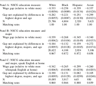
Nearly all non-Hispanic white men in the United States are native English speak-ers, while a substantial number of the women in our comparison groups are not. (See Borjas 1994 and Trejo 1997, for the relative importance of language skills for the earnings of immigrants.) In the final panel of Table 5, we conduct our same exercise but restrict attention to those individuals who report ‘‘speaking Table 5
Gender Wage Gaps Using Pre-Market Factors Only
Panel A: NSCG education measure White Black Hispanic Asian Wage gap (relative to white men) 20.333 20.258 20.339 20.337 (0.0056) (0.0089) (0.0134) (0.0120) Gap not explained by differences in
highest degree and age
20.282 20.221 20.251 20.299
(0.0055) (0.0087) (0.0130) (0.0121)
N 23,786 4,804 2,320 3,621
Matching rates 1.00 1.00 1.00 1.00
Panel B: NSCG education measure and major
Wage gap (relative to white men) 20.339 20.268 20.345 20.340 (0.0062) (0.0104) (0.0149) (0.0133) Gap not explained by differences in
highest degree, majors, and age
20.184 20.132 20.159 20.272
(0.0093) (0.0128) (0.0185) (0.0174)
N 20,622 4,188 2,024 3,106
Matching rates 0.867 0.872 0.872 0.858
Panel C: NSCG education measure and major, speak English at home Wage gap (relative to white men
whospeak English at home)
20.342 20.265 20.299 20.260
(0.0065) (0.0108) (0.0258) (0.0203) Gap not explained by differences in
highest degree, majors, and age
20.190 20.131 20.082 20.105
(0.0095) (0.0129) (0.0299) (0.0248)
N 19,095 3,917 645 950
Matching rates 0.860 0.866 0.888 0.859
Notes: The data are weighted to account for sample stratification. Estimates are from nonparametric regres-sions. All differentials are computed relative to white men. In Panel A, workers are matched on their age and NSCG-reported highest degree. In Panel B, we match workers on their age, NSCG-reported highest degree, and their highest degree major field of study. In Panel C, we match workers as in Panel B, but only those workers who speak only English at home. Bootstrapped standard errors are reported in parentheses based on 1,000 replications. Source: AuthorsÕcalculation, NSCG.
20. These inferences are drawn on the portion of the sample we were able to match, which is reasonably high here—nearly 87 percent in each demographic group.
English at home.’’21Limiting the sample to those respondents who speak English at home makes little difference in the estimates of the wage gaps for non-Hispanic white and black women. For Hispanic women the adjusted log wage gap declines to approximately 20.08 and for Asian women the gap falls to 20.11. For Asian and Hispanic women who speak English at home, well over half of the observed wage gap is explained by premarket factors age, highest degree, and major.
Our exact matching strategy is much more flexible than the usual parametric wage equations used for estimating gender wage gaps and is more parsimonious; we in-clude only three premarket covariates, and no market-related characteristics (indus-try, job characteristics, work attachment variables, et cetera) that are themselves potentially endogenous labor market outcomes. Yet, thanks to the level of detail in our education variables, our relatively parsimonious specification explains more of the gender wage gap than many other studies using extensive, and controversial, industry and occupation control variables.
B. The Role of Experience
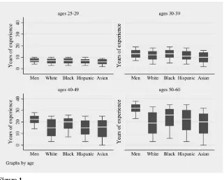
Even well-educated women have, on average, lower labor market attachment than men. Women are less likely than men to work full time on a roughly continuous basis over the course of their careers. To illustrate the differences, in Figure 1 we use a box-and-whiskers graph to plot the interquartile range (the box) and the 10th to 90th percentile range (the whiskers) of the experience measure for ages 25 to 29, 30 to 39, 40 to 49, and 50 to 60 for each of our five groups. The graph clearly shows that at the youngest ages there are few differences in experience by gender, but the differences grow monotonically with age. Not surprisingly, the wage gaps also grow monotonically with age. Using the same specification as in Table 5c, the wage gap is
20.09 for women of ages 25 to 29 years,20.24 for women of ages 30 to 39 years, 20.39 for women of ages 40 to 49, and20.43 for women of ages 50 to 60.22
At older ages, the support problem is quite severe. For instance, for the 50- to 60-year-old cohorts, the interquartile range of white men and white women no longer overlap and the median experience for women in this age group is below the 10th percentile of the white men’s distribution. Asian women have generally lower expe-rience levels than non-Hispanic white women, Hispanic women have similar experi-ence levels to non-Hispanic white women, and black women have higher experiexperi-ence levels than white women.
21. We do not match women who do not speak English at home with non-Hispanic white men who do not speak English at home for two reasons. First, because an overwhelming fraction of non-Hispanic white men speak English at home, we would only be able to match a small number of observations. More importantly, it is unclear whether language skills would be comparable for those we matched, particularly for Asian women. Most non-Hispanic white men who speak a language other than English at home speak another European language, which is probably closer linguistically to English than many Asian languages. Thus, we doubt whether such matches would represent workers of comparable English skills.
22. Interestingly, using British data, Manning and Swaffield (forthcoming) document that there is no wage gap at the time of labor market entry but that the gap increases to about 25 log points after just ten years of experience. Using US data on initial offer, McDonald and Thornton (2007) find that among holders of bach-elors’ degrees 95 percent of the wage gap is explained by majors selected at the time of entry into the labor market.
Decisions to temporarily leave the labor market are themselves potentially influ-enced by labor market outcomes—for example, disparate treatment in the workplace might influence some women to take leave from the labor market—and it is thus dif-ficult to know how to treat ‘‘experience’’ when estimating wage gaps. Here we focus on one approach that strikes us as sensible: We conduct an examination that is re-stricted to men and women who have ‘‘high labor market attachment.’’ We note in advance, though, that care must be taken in interpreting findings from this exercise (and below we supplement our main results with three alternate specifications that provide us with some additional evidence about the role of experience).
There are at least two reasons to focus on those with high labor market attachment. First, the work of Light and Ureta (1995) indicates that it is not only the quantity of experience but the timing of experience that affects wages. Because our data only allow us to measure the quantity of experience, we necessarily can compare only those individuals without (substantial) labor market interruptions. Second, because women and men have different reasons for labor market interruptions, it is far from clear that we should compare, say, a 40-year-old female accountant with a bachelor’s degree who had a 10-year labor market interruption to rear her children with a 40-year-old male accountant with a bachelor’s degree who had a 10-year labor mar-ket interruption because of a disability or a felony conviction.
Figure 1
Years of Work Experience for non-Hispanic White Men and Women (Non-Hispanic White, Black, Hispanic, and Asian) by Age
We implement our idea of ‘‘high labor market attachment’’ as follows: We form cells of men using age and highest degree, and then split these cells into smaller cells based on age, highest degree,and experience.23We retain for analysis only women and men with combinations of age, highest degree, and experience that contain more than 5 percent of the men from the corresponding cell formed on age and highest degree only. In short, we exclude a very small number of men who havemore expe-rience than most other men, a somewhat larger number of men who have abnormally low levels of experience given their age and highest degree, and a larger proportion yet of women with relatively low levels of experience. Thus in our matching exercise we are including only those women who have the roughly the same levels of expe-rience as ‘‘typical’’ men.24
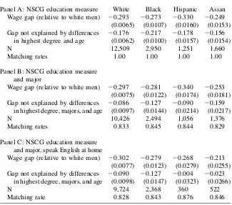
Table 6 presents results of this exercise. Panel A shows that in this sample of indi-viduals with high labor market attachment, there are still large raw wage gaps and substantial gaps not explained by highest degree and age. In Panel B we match work-ers on their age, highest degree, and major. In Panel C we repeat the exercise limiting our sample to those who speak English at home. For both Asian and Hispanic women the unexplained wage gap falls dramatically and is no longer statistically signifi-cant. Unexplained wage gaps are somewhat higher for non-Hispanic white and black women, but, at20.09 and 20.13 respectively, are considerably smaller than
raw gaps.
In forming the comparisons reported in Table 6, we are using data from only about half of the women in our sample (compare sample sizes in Tables 5 and 6). We are simply unable to draw inferences about wage gaps for a large group of women— primarily women with relatively lower labor market attachment. One alternative strategy is to match on experience, age, degree, and field of study forallwomen, including those with atypical work experience patterns. We do not report results from this exercise in the tables, but they are well within one standard error of the estimates in the last line in Panel C of Table 6. In forming these estimates, match-ing rates are quite low, between 0.35 and 0.40, so inferences are bematch-ing drawn for a relatively small, not necessarily representative, subsample. A second alternative is to make a strong Mincerian assumption and match on experience (and education) but not age. This specification again gives similar estimates,20.10 and20.11 for
non-Hispanic white and black women, and 20.08 and 20.04 for Hispanic and Asian women who speak English at home (with matching rates of between 83 and 85 percent).
A third alternative is to conduct a match in which we restrict attention to unmar-ried childless women. The idea behind this exercise is motivated by Becker (1985), who argues that even conditioning on labor market experience may not be sufficient to control for differences in labor force commitment. Becker argues that if women
23. The NSCG includes measures of full-time experience, gathered retrospectively as of April 1993 (rather than 1989, as are earnings). Of course this retrospective question may contain much measurement error, an issue we ignore here.
24. Using this approach, however, we are unable to match a considerable number of women who have sig-nificant interruptions in their careers. This lack of a common support is a common problem with matching estimators; see Heckman, Ichimura, Smith, and Todd (1998) and Heckman, Ichimura, and Todd (1998) for a more detailed discussion. Our trimming, based on the conditional distribution of experience, is similar in spirit to trimming based on the propensity score used in Heckman, Ichimura, Smith, and Todd (1998).
specialize in home production, men and women with identical abilities and years of full-time experience may have different labor market outcomes owing to differing choices of time and effort allocation. Restricting attention to unmarried women who do not have children—women who are less likely to specialize away from mar-ket production—may allow us to circumvent this issue. Once matches are made based on age, highest degree, and major and the sample is restricted to those who speak English at home, estimated wage gaps for Hispanic and Asian women relative to white men again do not differ significantly from zero, and the log wage gaps for white and black women are approximately20.07 and20.09 respectively.
Table 6
Gender Wage Gaps for Those with High Labor Market Attachment
Panel A: NSCG education measure White Black Hispanic Asian Wage gap (relative to white men) 20.293 20.273 20.330 20.249 (0.0065) (0.0107) (0.0160) (0.0153) Gap not explained by differences
in highest degree and age
20.176 20.217 20.178 20.156
(0.0062) (0.0100) (0.0157) (0.0154)
N 12,509 2,950 1,251 1,660
Matching rates 1.00 1.00 1.00 1.00
Panel B: NSCG education measure and major
Wage gap (relative to white men) 20.297 20.281 20.340 20.253 (0.0075) (0.0122) (0.0174) (0.0181) Gap not explained by differences
in highest degree, majors, and age
20.086 20.127 20.090 20.159
(0.0097) (0.0144) (0.0214) (0.0217)
N 10,426 2,494 1,056 1,376
Matching rates 0.833 0.845 0.844 0.829
Panel C: NSCG education measure and major, speak English at home
Wage gap (relative to white men) 20.302 20.279 20.268 20.213 (0.0077) (0.0123) (0.0279) (0.0255) Gap not explained by differences
in highest degree, majors, and age
20.090 20.127 20.004 20.023
(0.0098) (0.0147) (0.0323) (0.0266)
N 9,724 2,368 360 522
Matching rate 0.828 0.843 0.876 0.846
Notes: The data are weighted to account for sample stratification. Estimates are from nonparametric regres-sions. In Panel A, workers are matched on their age and NSCG-reported highest degree. In Panel B, we match workers on their age, NSCG-reported highest degree, and majors. In Panel C, we match workers as in Panel B, but only those workers who speak only English at home. Bootstrapped standard errors are reported in parentheses based on 1,000 replications. The sample is limited to women (and men) who are in an age-highest degree-full time experience category that holds more than 5 percent of the white males in that age-highest degree category. Source: AuthorsÕcalculation, NSCG.
C. Comparison of Nonparametric and Parametric Results
As discussed above, empirical studies of the gender wage gap generally use linear regression. Data sets with detailed data on education, labor market experience, and other human capital measures are often relatively small. Thus, researchers have found it useful to make parametric restrictions within a regression framework as a practical way to gain precision in making inferences about the gender wage gap. It is therefore of some interest to examine the extent to which the results we report in Table 6 differ from those one would find using the standard linear regression approach—making parametric restrictions that researchers typically use when work-ing with smaller data sets.25This exercise helps us isolate the gains from the added flexibility of nonparametric estimation that our larger data set affords.
We continue to use as our sample four racial/ethnic groups of women and non-Hispanic white men. We run the two most typical types of parametric models, as described in Section III—models in which coefficients are pooled across groups (but dummy variables capture an intercept shift), and models that are run separately for each demographic group. Our linear regression models include dummy variables for each of the 144 possible fields of study, dummy variables for degree, a quadratic in age, a quadratic in years of full-time experience, and an indicator for whether the respondent speaks English at home. By running separate regressions for each racial/ethnic group, and by including 144 possible fields of study, we allow for more flexibility than is common in the gender wage gap literature.
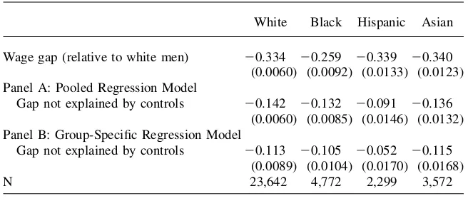
Table 7 presents the resulting estimated wage gaps—estimates that are directly comparable to those given in Panel C of Table 6. In the linear regression approaches, the unexplained log wage gap of20.11 to20.13 for black women is similar to the
20.13 gap we estimate using nonparametric methods. For white women, though, the
parametric estimates of20.11 to20.14 are somewhat larger than the20.09 mate from the nonparametric approach. More strikingly, the regression-based esti-mates of the unexplained gap for Hispanic women (20.05 to 20.09) and Asian women (20.12 to 20.14) are quite different from the nonparametric estimates of 20.004 and20.02 respectively.
D. An Additional Exploration of the Black-White Wage Gap
In our analyses that use exclusively premarket factors we consistently estimate that the wage gap for non-Hispanic white women is larger than the gap for non-Hispanic black women. Once we condition on labor market experience by restricting the sam-ple to men and women with high labor market attachment, however, the gap for white women drops below that of black women. This finding parallels analysis by Neal (2004), who demonstrates that estimates of the wage gap between black and white women are understated when one assumes that labor market participation rates are similar between the groups. Neal shows, in fact, that well-educated black women have higher labor market attachment than corresponding white women, whereas the reverse is true for black and white women with low educational levels.
25. In principle regression models can be made parametrically flexible; for example, a fully saturated re-gression model (that is, a model with all possible interactions of independent variables) would be equivalent to our nonparametric approach. Our purpose is to explore the sensitivity of results to common restrictions adopted in the literature.
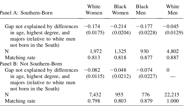
In our empirical investigation of college-educated women, when we restrict atten-tion to women with high labor market attachment, black women have the lowest wages of any demographic group, with a log wage gap of 20.13 relative to non-Hispanic white men. This finding motivates an additional examination of the wage disparities for black and white women. In particular, we conduct separate gender and racial wage gap analyses for men and women born in the South and born else-where in the country (loosely defined as the ‘‘North’’). We speculate that there may be a relatively larger gap for Black women born in the South stemming in part from a wide racial disparity in educational opportunity.26Card and Krueger (1992) docu-ment that especially for school children born prior to 1940 (who would be among the older workers in our sample, or would be parents of the younger workers in our sample), the quality of the segregated public schools in much of the Southern United States was much worse for blacks than for whites.27 At the college level, Daniel, Black, and Smith (2001) note that many historically black institutions of higher education, particularly in the South, rank very low along a number of tradi-tional measures of educatradi-tional quality. Using evidence provided in Ehrenberg and Rothstein (1993, Table 2) from the NLS Class of 1972, we calculate that among blacks attending college, 66 percent of those born in the South attended a Table 7
Parametric Gender Wage Gaps by Race and Ethnicity
White Black Hispanic Asian Wage gap (relative to white men) 20.334 20.259 20.339 20.340
(0.0060) (0.0092) (0.0133) (0.0123) Panel A: Pooled Regression Model
Gap not explained by controls 20.142 20.132 20.091 20.136 (0.0060) (0.0085) (0.0146) (0.0132) Panel B: Group-Specific Regression Model
Gap not explained by controls 20.113 20.105 20.052 20.115 (0.0089) (0.0104) (0.0170) (0.0168)
N 23,642 4,772 2,299 3,572
Notes: The data are weighted to account for sample stratification. Covariates are age and age squared, de-gree, three-digit major, years of full time experience and experience squared, and an indicator for a lan-guage other than English spoken at home. There are 39,938 white men used in the regressions. Source: AuthorsÕcalculation, NSCG.
26. We define Southern states as Alabama, Arkansas, Florida, Georgia, Kentucky, Louisiana, Mississippi, Missouri, North Carolina, South Carolina, Tennessee, Texas, and Virginia. (We refer to individuals born elsewhere as being ‘‘not born in the South’’ or as ‘‘Northern-born.’’) In Black, Haviland, Sanders, and Taylor (2006), which studies race and ethnic wage gaps among college-educated men, we similarly find that the gap (relative to non-Hispanic white men) is higher for black men than for Asian and Hispanic men. 27. For example, blacks in the 1920-1929 birth cohort who attended public schools in Alabama, Georgia, Louisiana, Mississippi, or South Carolina typically were in classes that were 30 to 50 percent larger than those of white students and received instruction from teachers who earned less than half as much as teachers in white schools.