Air Quality and Early-Life Mortality
Evidence from Indonesia’s Wildfires
Seema Jayachandran
a b s t r a c t
Smoke from massive wildfires blanketed Indonesia in late 1997. This paper examines the impact that this air pollution (particulate matter) had on fetal, infant, and child mortality. Exploiting the sharp timing and spatial patterns of the pollution and inferring deaths from ‘‘missing children’’ in the 2000 Indonesian Census, I find that the pollution led to 15,600 missing children in Indonesia (1.2 percent of the affected birth cohorts). Prenatal exposure to pollution drives the result. The effect size is much larger in poorer areas, suggesting that differential effects of pollution contribute to the
socioeconomic gradient in health.
I. Introduction
Between August and November 1997, forest fires engulfed large parts of Indonesia, destroying over 12 million acres. Most of the fires were started intentionally by logging companies and palm oil producers clearing land to plant new crop.1Because of the dry, windy conditions caused by El Nin˜o, the fires burned out of control and spread rapidly. In November, rains finally doused the fires.
Seema Jayachandran is an assistant professor of economics at Stanford University and a faculty research fellow at the National Bureau of Economic Research. She is grateful to Doug Almond, Janet Currie, Erica Field, Dan Kammen, Michael Kremer, Doug McKee, Ben Olken, Sarah Reber, Duncan Thomas, seminar participants at AEA, Berkeley, BREAD, Columbia, Maryland, Stanford GSB, UCLA, and Harvard/MIT/BU, and three anonymous referees for helpful comments. She also thanks Kok-Hoe Chan and Daniel Chen for data and Nadeem Karmali and Rika Christanto for excellent research assistance. The data used in this article are available for purchase through the Indonesian Statistics Bureau (Badan Pusat Statistik). The author will assist other scholars who have purchased the data to reproduce the data set used here. Contact jayachan@stanford.edu.
½Submitted December 2006; accepted May 2008
ISSN 022-166X E-ISSN 1548-8004Ó2009 by the Board of Regents of the University of Wisconsin System
T H E J O U R NA L O F H U M A N R E S O U R C E S d 4 4 d 4
While the fires were burning, much of Indonesia, especially Sumatra and Kalimantan where the fires were concentrated, was blanketed in smoke. This paper examines fetal, infant, and child mortality caused by the episode of poor air quality (specifically, high levels of particulate matter). Daily satellite measurements of airborne smoke at locations across Indonesia provide information on the spatial and temporal patterns of the pollution. The outcome is fetal, infant, and child mortality before age three—hereafter called early-life mortality—and is inferred from ‘‘missing children’’ in the 2000 Census, overcoming the lack of mortality records for Indonesia and the small samples in surveys with mortality data.
The paper finds that higher levels of pollution caused a substantial decline in the size of the surviving cohort, and that exposure to pollution during the last trimester in utero is the most damaging. The fire-induced increase in air pollution is associ-ated with a 1.2 percent decrease in cohort size. This estimate is the average across Indonesia for the five birth-month cohorts with high third-trimester exposure to pollution; it implies that 15,600 child, infant and fetal deaths are attributable to the pollution. Indonesia’s under-three mortality rate during this period was about 6 percent; if the estimate is driven mainly by child and infant deaths (rather than fetal deaths), this represents a 20 percent increase in under-three mortality.
The paper also finds a striking difference in the mortality effects of pollution between richer and poorer places. Pollution has twice the effect in districts with be-low-median consumption compared to districts with above-median consumption. Individuals in poorer areas could be more susceptible to pollution because of lower baseline health, more limited options for avoiding the pollution, or less access to medical care. Another possibility is that people exposed to indoor air pollution on a daily basis suffered more acute health effects from the wildfires because they re-ceived a double dose of pollution. Consistent with this view, the effects are larger in areas where more people cook with wood-burning stoves. Surprisingly, mother’s education does not seem to play a role. While these correlations do not pin down causal relationships, they provide suggestive evidence on why the poor are especially vulnerable to the health effects of pollution and add to our understanding of the so-cioeconomic (SES) gradient in health (Marmotet al.1991; Smith 1999). An open question in the literature is how much of the health gradient is due to low-SES indi-viduals being more likely to suffer adverse health shocks and how much is due to a given health shock having worse consequences for the poor (Case, Lubotsky, and Paxson 2002; Currie and. Hyson 1999). This paper provides some evidence for the second mechanism: People faced a common environmental-cum-health shock, and the consequences were much worse for the poor.
This study examines an extreme episode of increased pollution, which has advan-tages for empirical identification. The abruptness and magnitude of the pollution are useful for identifying when in early life exposure to pollution is most harmful. In utero exposure is found to be especially important, suggesting that targeting pregnant women should be a priority of public health efforts concerning air pollution. The extreme level of pollution, however, also means that one must be cautious about ex-trapolating the effect size to more typical levels of pollution.
That being said, rampant wildfires are not uncommon in Indonesia and other coun-tries, mainly in Southeast Asia and Latin America, where fire is used to clear land. Most cost estimates of the 1997 Indonesian fires have focused on destroyed timber,
reduced worker productivity, and lost tourism and are in the range of $2 to 3 billion (Tacconi 2003). This study shows that the health costs of the fires are much larger: Assuming a value of a statistical life of $1 million, the early-life mortality costs alone were over $15 billion.2The costs of the fires very likely overwhelm the benefits to firms from setting them; the annual revenue from Indonesia’s timber and palm oil industries at this time was less than $7 billion.
The remainder of the paper is organized as follows. Section II provides back-ground on the link between pollution and health and on the Indonesian fires. Section III describes the data and empirical strategy. Section IV presents the results, and Section V concludes.
II. Background
A. Link between air pollution and early-life mortality
1. Related Literature
Previous related work includes that by Chay and Greenstone (2003b), who use variation across the United States in how much the 1980–81 recession lowered pol-lution and find that better air quality reduced infant mortality. Chay and Greenstone (2003a) also find that pollution abatement after the Clean Air Act of 1970 led to a decline in infant deaths.3Currie and Neidell (2005), in their study of California in the 1990s, find that exposure to carbon monoxide and other air pollutants during the month of birth is associated with infant mortality.4
In addition, there have been studies on the adult health effects of Indonesia’s 1997 fires. Emmanuel (2000) finds no increase in mortality but an increase in respiratory-related hospitalizations in nearby Singapore. Sastry (2002) finds increased mortality for older adults on the day after a high-pollution day in Malaysia. Frankenberg, Thomas, and McKee (2004) compare adult health outcomes in 1993 and 1997 for areas in Indonesia with high versus low exposure to the 1997 smoke. They find that pollution reduced people’s ability to perform strenuous tasks and other measures of health. Their data set covers 321 of the 4,000 subdistricts in Indonesia, and only one of Kalimantan’s four provinces is in their sample. Thus, one advantage of this paper is its broader geographic coverage, which allows one to explore hetero-geneous effects and nonlinearities in the health impact of pollution, for example.
2. This value of a statistical life (VLS) is calculated using $5 million in 1996 dollars as the value for the United States from Viscusi and Aldy (2003), Murphy and Topel (2006), and the U.S. Environmental Pro-tection Agency (2000); an income elasticity of a VSL of 0.6 from Viscusi and Aldy (2003); and the fact that Indonesia’s per capita gross domestic product was one tenth of U.S. GDP. Note that the total health costs from early-life exposure to the pollution would also include costs among those who survived. Recent work suggests that there could be long-term consequences among surviving fetuses (Barker 1990; Almond 2006). 3. Other natural experiments used to measure health effects of air pollution include the temporary closure of a steel mill in Utah during a labor dispute; the reduction in traffic during the 1996 Olympics in Atlanta; and involuntary relocation of military families (Pope, Schwartz, and Ransom 1992; Friedmanet al.2001; Lleras-Muney 2006).
4. For research on pollution and infant mortality outside the United States, see, for example, Bobak and Leon (1992) on the Czech Republic, Loomiset al.(1999) on Mexico, and Her Majesty’s Public Health Ser-vice (1954) on the 1952 London ‘‘killer fog’’ episode.
Another important advance over previous work is the use of both the sharp timing and extensive regional variation of the pollution; one can then identify causal effects while allowing for considerable unobserved heterogeneity across time and place.
2. Physiological Effects of Pollution
Smoke from burning wood and vegetation, or biomass smoke, consists of very fine particles (organic compounds and elemental carbon) suspended in gas. Fine par-ticles less than 10 microns (mm) and especially less than 2.5mm in diameter are considered the most harmful to health because they are small enough to be inhaled and transported deep into the lungs. For biomass smoke, the modal size of particles is between 0.2 and 0.4mm, and 80 to 95 percent of particles are smaller than 2.5mm (Hueglinet al.1997).
Prenatal and postnatal exposure to air pollution could affect fetal or infant health through several pathways. Postnatal exposure can contribute to acute respiratory in-fection, a leading cause of infant death. Prenatal exposure can affect fetal develop-ment, first, because pollution inhaled by the mother interferes with her health, which in turn disrupts fetal nutrition and oxygen flow, and, second, because toxicants cross the placenta. Several studies find a link between air pollution and fetal growth retardation or shorter gestation period, both of which are associated with low birth-weight (Dejmeket al.1999; Wanget al.1997; Berkowitzet al.2003). The biological mechanisms behind these pregnancy outcomes are related to the main toxicant in particulate matter, polycyclic aromatic hydrocarbons (PAHs). In utero exposure to particulate matter has been associated with a greater prevalence of PAH-DNA adducts on the placenta, and PAH-DNA adducts, in turn, are correlated with low birth weight, small head circumference, preterm delivery, and fetal deaths (Pereraet al. 1998; Hatch, Warburton, and Santella 1990). Laboratory experiments on rats have confirmed most of these effects (Rigdon and Rennels 1964; MacKenzie and Ange-vine 1981). PAHs disrupt central nervous system activity of the fetus, and during crit-ical growth periods such as the third trimester, the disruption has a pronounced effect on fetal growth. PAHs are also hypothesized to reduce nutrient flow to the fetus by suppressing estrogenic and endocrine activity and by binding to placental growth factor receptors (Pereraet al.1999).
B. Description of the Indonesian Fires
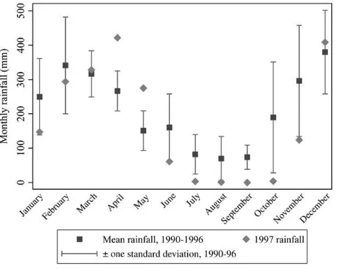
The 1997 dry season in Indonesia was particularly dry. Figure 1 shows the monthly rainfall recorded at a meteorological station in South Sumatra in 1997 compared to previous years. The 1997 dry season was both severe and prolonged: Rainfall amounts in June to September were lower than usual, and the rainy season was delayed until November. The rest of Indonesia experienced rainfall patterns similar to Sumatra’s.
Fires are commonly used in Indonesia to clear land for cultivation, and the dry sea-son is considered an opportune time to set fires because the vegetation burns quickly. Industrial farmers burn forest land in order to replant it with palm or timber trees, and small farmers use ‘‘slash–and–burn’’ techniques in which land is cleared with fire to ready it for cultivation. In addition, logging companies are thought to have set some
virgin forests on fire since the government would then designate the degraded land as available for logging.
With expansion of the timber and palm oil industries in Indonesia, many tracts of forest land have become commercially developed, and logged-over land is more prone to fires than pristine forest.5 Roads running through forests act as conduits for fire to spread, and with the canopy gone, the ground cover becomes drier and more combustible and wind speeds are higher. Also, because logging firms were taxed on the volume of wood products that left the forest, they often left behind waste wood, even though it had economic value as fertilizer or wood chips. The left-behind debris wood made the forest more susceptible to fast-spreading fires (Barber and Schweithhelm 2000).
In September 1997, because of the dry conditions, the fires spread out of control. The Indonesian government made some attempt to fight the fires, but the efforts were ineffective. The fires continued until the rains arrived in November. The fires were concentrated in Sumatra and Kalimantan. About 12 million acres were burned, 8 million acres in Kalimantan (12 percent of its land area) and four million in Suma-tra (4 percent of its area). The practice of clearing land with fire is used throughout Indonesia, and El Nin˜o affected all of Indonesia. What set Sumatra and Kalimantan apart is that Indonesia’s forests are mainly in these areas. The majority of crop plan-tations are located in Sumatra, and planplan-tations are a fast-growing use of land in Kali-mantan. Timber operations are also primarily in these regions.
Figure 1
Rainfall at Palembang Airport meteorological station, South Sumatra, 1990-97
5. In 1996 forest products accounted for 10 percent of Indonesia’s gross domestic product, and Indonesia supplied about 30 percent of the world palm oil market (Ross 2001).
The location of the smoke generally tracked the location of the fires, though because of wind patterns, not entirely. Fires were concentrated on the southern parts of Sumatra and Kalimantan, and these two areas experienced the most pollution. On the other hand, the northern half of Sumatra was strongly affected by smoke while Java was relatively unaffected, yet neither of these areas experienced fires, for example.
A common measure of particulate matter is PM10, the concentration of particles less than ten mm in diameter. The U.S. Environmental Protection Agency has set a PM10standard of 150 micrograms per cubic meter (mg/m3) as the 24-hour average that should not be exceeded in a location more than once a year. During the 1997 fires, the pollution in the hardest hit areas surpassed 1000mg/m3 on several days and exceeded 150mg/m3 for long periods (Ostermann and Brauer 2001; Heil and Goldammer 2001). The pollution levels caused by the wildfires are comparable to levels caused by indoor use of wood-burning stoves. The daily average PM10level from wood-burning stoves, which varies depending on the dwelling and duration of use, ranges from 200 to 5000mg/m3(Ezzati and Kammen 2002).
III. Empirical Strategy and Data
A. Empirical Model and Outcome Variable
The goal of the empirical analysis is to measure the effect that air pollution from the wildfires had an on early-life mortality. Ideally, there would be data on all preg-nancies indicating which ended in fetal, infant, or child death, and the following equation would be estimated:
Survivejt¼b1Smokejt+dt+aj+ejt:
ð1Þ
The variableSurvivejtis the probability that fetuses whose due date is monthtand whose mothers reside at the time of the fires in subdistrictjsurvive to a certain point, such as live birth, one year, etc. The prediction is thatb1is negative, or that exposure to smoke around the time of birth reduces the probability of survival.
In practice, mortality records are unavailable for Indonesia, and survey samples are too small to examine the effects of month-to-month fluctuations in pollution. For example, the 2002 Demographic and Health Survey has on average one birth and 0.05 recorded child deaths per district-month for the affected cohorts.6Therefore, the approach I take is to infer early-life mortality by measuring ‘‘missing children.’’ The outcome measure is the cohort size for a subdistrict-month calculated from the complete 2000 Census of Population for Indonesia. The estimating equation is
lnðCohortSizeÞjt¼b1Smokejt+b2PrenatalSmokejt+b3PostnatalSmokejt+dt+aj+ejt
ð2Þ
The dependent variable, ln(CohortSize)jt, is the natural logarithm of the number of people born in monthtwho are alive and residing in subdistrictjat the time of the 2000
6. Appendix 1 verifies that population counts from the Census move one-for-one with births and deaths in the Demographic and Health Survey sample.
Census. Smokejt is the pollution level in the month of birth, and PrenatalSmokejt andPostnatalSmokejtare the pollution level before and after the month of birth. Each observation is weighted by the subdistrict’s population (the number of people enumer-ated in the Census who were born in the two years prior to the sample period).
An advantage of the Census compared to a survey is that the data are for the entire population. Also, the outcome variable measures fetal deaths in addition to infant and child deaths, albeit without distinguishing between the different outcomes; most surveys do not collect data on fetal deaths. Finally, population counts are often better measured than infant and child mortality because of underreporting of deaths and recall error on dates of deaths.
There are several potential concerns about inferring mortality from survivors, however. Since the data come from a cross-section of survivors in June 2000, the outcome represents a different length of survival for individuals born at different times, and the mean level of survival will differ by cohort, independent of the fires. For a cohort born in December 1997 around the time of the fires, the outcome is sur-vival until age two and a half, while for an older cohort born in December 1996, the outcome is survival until age three and a half, for example.7The inclusion of birthyear-birthmonth (hereafter, month) fixed effects in the regression will control for any average differences in survival by cohort.
In using ln(CohortSize) as a proxy for the early-life mortality rate, an assumption is that, conditional on subdistrict and month fixed effects, pollution is not correlated with ln(Births). This seems like a reasonable assumption. First, by using a short panel, subdistrict fixed effects absorb most variation in the number of women of childbearing age and other determinants of fertility. Month effects control for fertility trends and seasonality. Second, it seems unlikely that there were large fluctuations in fertility that coincided with the air pollution both spatially and temporally. Even area-specific trends could not explain the patterns since the sample includes control periods both before and after the fires; any omitted fertility shift causing bias would have to be a short-term downward or upward spike in particular regions. In addition, Section IVB provides empirical evidence that fertility is unlikely to be a confounding factor.
Another concern is that if pollution affects the duration of pregnancies, then miss-ing children might result from the shiftmiss-ing of births from certain months to other months. If exposure to smoke induces preterm labor, then one would expect to see an excess of births followed by a deficit of births. In Section IVB, I examine and am able to reject that the results are an artifact of changes in gestation period.
There are also potential empirical concerns not unique to using ln(CohortSize) as the dependent variable. First, pollution might affect not only mortality but also fer-tility. This would influence the population counts for the later ‘‘control’’ cohorts and could lead to sample selection problems even if mortality were directly measured. I therefore restrict the sample to births occurring no more than eight months after the outbreak of the fires, or cohorts who were conceived before the fires. Second, the empirical model assumes that exposure to pollution just before or after birth affects mortality, an assumption motivated by previous findings. However, exposure
7. One advantage of observing survival more than two years after the due date is that for deaths that occur around birth, the estimates are less likely to reflect simply short-term ‘‘harvesting.’’
to pollution earlier in a pregnancy or later after birth also could affect health. If the control cohorts are in fact also treated, though less intensely, then the results would underestimate the true effects.
A third important concern arises from the fact that individuals are identified by their subdistrict of residence in 2000 rather than the subdistrict where their mother resided during the end of her pregnancy or just after giving birth. If families living in high-smoke areas with children born around the time of the fires were more likely to leave the area (either during or after the fires), then the cohort size would be smaller in areas more affected by pollution. Fortunately, one can directly examine this concern since the Census collects the district of birth and the district of residence in 1995. As discussed in Section IVB, the results are identical using birthplace, current location, or mother’s location in 1995.
Table 1 presents the descriptive statistics. The sample comprises monthly observa-tions between December 1996 and May 1998 (18 months) for 3,751 subdistricts (kecamatan). Of this starting sample size of 67,518 observations, 64 observations are dropped because the cohort size for the subdistrict-month is 0.8 There are on average 96 surviving children per observation. The larger administrative units in Indonesia are districts (kabupaten), of which there are 324 in the sample, and prov-inces, of which there are 29.
B. Pollution Variable
The measure of air pollution is the aerosol index from the Earth Probe Total Ozone Mapping Spectrometer (TOMS), a satellite-based monitoring instrument. The aero-sol index tracks the amount of airborne smoke and dust and is calculated from the optical depth, or the amount of light that microscopic airborne particles absorb or reflect. The TOMS index has been found to quite closely track particulate levels mea-sured by ground-based pollution monitors (Hsuet al.1999). Ground monitor data are not available for Indonesia for this period. The aerosol index runs from22 to 7, with a higher index indicating more smoke and dust.
The TOMS data contain daily aerosol measures (which are constructed from observations taken over three days) for points on a 1 degree latitude by 1.25 degree longitude grid. Adjacent grid points are approximately 175 kilometers (km) apart. The probe began collecting data in mid-1996, and the data I use begin in September 1996. For each subdistrict, I calculate an interpolated daily pollution measure that combines data from all TOMS grid points within a 100-km radius of the geo-graphic center of the subdistrict, weighted by the inverse distance between the sub-district and the grid point. The number of TOMS grid points that fall within the catchment area of a subdistrict ranges from one to six and is on average four. The mean distance between a subdistrict’s center and the nearest grid point is 50 km.
8. The Census covers 3,962 subdistricts that make up 336 districts. For subdistricts dropped from the sam-ple, either the latitude and longitude could not be determined or there were no enumerated children for more than 15 percent of the monthly observations due to missing data or very small subdistrict size. In ad-dition, I drop four districts that make up Madura since this area received a large influx of return migrants in 1999 in response to ethnic violence against them in Kalimantan, and also Aceh province where separatist violence is thought to have affected the quality of the Census enumeration. The results are robust to drop-ping Irian Jaya, another area where unrest could have affected data quality.
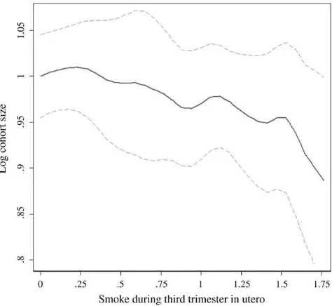
Table 1
Descriptive Statistics
Mean Std. Dev.
Cohort size variables
Cohort size (for subdistrict-month) 95.6 89.7
Ln(cohort size) 4.8 0.8
Pollution variables
Smoke (median daily value for month) 0.087 0.424 Prenatal smoke (Smoket-1,2,3) 0.095 0.330
Postnatal smoke (Smoket+1,2,3) 0.074 0.342
Proportion of days with high smoke (aerosol index > 0.75) 0.047 0.154 Average smoke (daily values averaged for the month) 0.120 0.445
Mean of smoke for Aug-Oct 1996 0.048 0.069
Mean of smoke for Aug-Oct 1997 0.578 0.791
Mean of prenatal smoke for Sept 1996–Jan 1997 0.038 0.052 Mean of prenatal smoke for Sept 1997–Jan 1998 0.341 0.522 Other variables
Fires (any fires) 0.157 0.364
Intense fires (number x duration of fires$10 fire-days) 0.026 0.157 Rainfall for June to November 1997 relative to 1990–95 0.480 0.241 Ln(median 1996 household food consumption) 10.52 0.26
75th percentile 10.71
50th percentile 10.49
25th percentile 10.33
Median HH food consumption in 1996 / Median HH food consumption in 1998
0.742 0.070
National consumer price index (for food) 1.131 0.202
Urbanization 0.57 0.39
Wood as primary cooking fuel 0.636 0.413
Doctors per 1,000 people 0.161 0.241
Maternity clinics per 1,000 people 0.031 0.050 Educated mothers (completed junior high) 0.386 0.215
Note: The sample consists of 67,454 subdistrict-birthmonths from December 1996 to May 1998. Sample averages are weighted by population (the number of people enumerated in the Census born in the year be-fore the sample period), except for cohort size for which the unweighted mean is shown. Cohort size is the number of people enumerated in the 2000 Census who were born in a subdistrict in a given month. Smoke is the monthly median of the daily TOMS aerosol index which is interpolated from TOMS grid points within 100 km of the subdistrict’s geographic center and weighted by the inverse distance between the grid point and subdistrict center. Prenatal and Postnatal Smoke are averages of Smoke for the three months be-fore and after the month of birth. Fire-days is calculated from European Space Agency hot spots within 50 km of the subdistrict’s center. Rainfall is measured at the nearest grid point on a 0.5 degree latitude/longi-tude grid and is the mean of 1997 rain relative to 1990–95 for June to November. Urbanization is the sub-district’s percent of births in urban areas based on those born 1994–96 and uses an indicator in the Census of whether the respondent’s locality is rural or urban. Educated mothers is the percent of infants whose mother has completed junior high and is based on matching infants to mothers in the Census. Median food consumption is a per capita measure for each district that uses data from the 1996 and 1999 SUSENAS household survey. Consumer price index is from the Indonesian central bank. Healthcare variables are cal-culated for each subdistrict using the 1996 PODES (survey of village facilities). PODES and SUSENAS data are available for 63,158 observations.
The monthly measure is calculated as the median of the daily values, and I also use the mean of the daily values and the number of days that exceed a threshold value of 0.75.
The data include more than 3,700 subdistricts, but only 226 unique pollution grid points used. Interpolation adds spatial variation at a finer grain, but uncorrected stan-dard errors would nevertheless overestimate how much independent variation there is in the pollution measure. Moreover, the actual pollution level is spatially correlated. Therefore I allow for clustering of errors among observations within an island group by month. The sample has ten island groups (Sumatra, Java, Sulawesi, Kalimantan, Bali, West Nusa Tenggara, East Nusa Tenggara, Irian Jaya, Maluku, and North Maluku).9
The estimating Equation 2 includes pollution in the month of birth (Smokejt) as well as lags ofSmokejtwhich measure exposure to pollution in utero, and leads that measure exposure after birth. Note thatSmokejtmeasures both prenatal and postnatal exposure, with the balance depending on when in the calendar month an individual is born (the Census did not collect the specific date of birth, only the month). It becomes difficult to separately identify each lag and lead with precision, so the main specification uses an average of the pollution level for the three months before the birth month (PrenatalSmokejt) and after the birth month (PostnatalSmokejt). The pop-ulation-weighted mean values ofSmoke,PrenatalSmoke, and PostnatalSmoke are 0.09, 0.10, and 0.07, as shown in Table 1. On average, the pollution index exceeds 0.75 on 5 percent of days.
During the months of the fires, August to October 1997, the mean aerosol index for Indonesia was 0.58. For the same months in 1996, the mean was 0.05. Similarly, the mean ofPrenatalSmokewas 0.34 for the most affected cohorts (births in Septem-ber 1997 to January 1998) while during the same months a year earlier, the mean was 0.04. These gaps are helpful when interpreting the regression coefficients and quan-tifying the impact of the fires.
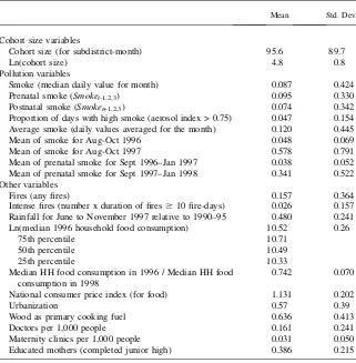
The intensity of smoke varied across Indonesia. Figure 2a shows the coefficients on island-specific month fixed effects for Kalimantan and Sumatra, the hardest hit regions. The pollution was most severe during August to October 1997, both for Indonesia as a whole and in relative terms for Kalimantan and Sumatra, as shown. Kalimantan expe-rienced another episode of smoke in early 1998 after the rainy season ended.
Figure 2b plots the corresponding island-specific month effects using log cohort size as the outcome variable. Intuitively, the identification strategy is to test whether in the areas most affected by the pollution, the size of cohorts that were born around the time of the pollution is abnormally low. The regression analysis uses not only this between-island variation but also within-island variation. Even using just this coarse variation, one can see in the point estimates the decline in cohort size for the affected island-months.
C. Other Variables
Several other variables are used either as controls or to examine differential effects of pollution (that is, as interaction terms). First, I construct a measure of the financial
9. The standard errors are almost identical if they are clustered on island, suggesting that serial correlation is not a major concern. However, using only ten clusters is not advisable since ‘‘the cluster approach may be quite unreliable except in the case where there are many groups’’ (Donald and Lang 2007).
crisis that hit Indonesia in late 1997. Cross-sectional variation in the crisis is mea-sured as the 1996 to 1999 ratio of the median log food consumption per capita in a district; the value is higher in areas hit harder by the crisis. The consumption data are from the National Socioeconomic Survey (SUSENAS), a household survey con-ducted annually by the national statistics bureau. The survey is representative at the district rather than subdistrict level, so data are aggregated to the district. The data Figure 2
Pollution and Log Cohort Size by Month and Location
Note:This figure plots coefficients and standard errors from a regression of A. pollution and B. log cohort size on subdistrict and month fixed effects and island-specific month fixed effects for Kaliman-tan and Sumatra. The month fixed effects for KalimanKaliman-tan and Sumatra are plotted. The vertical lines delineate the three months of highest pollution in A and the six birth cohorts that experienced high pollution in the month of birth or third trimester in utero in B.
appendix (Appendix 2) describes in more detail how the consumption measure is constructed. The national consumer price index for food is from the central bank and is used as a measure of temporal variation in the crisis. The interaction of these two variables is the crisis measure.
The cross-sectional consumption measure for 1996 is interacted with the pollution variables to examine how the effects of pollution differ for rich and poor areas. Healthcare measures such as doctors and maternity clinics per capita, as well as the type of fuel people cook with are from the 1996 Village Potential Statistics (PODES), a census of community characteristics. The PODES has an observation for each of over 66,000 localities, which I aggregate to the subdistrict level. In the analyses that use data from the PODES or SUSENAS, the sample size is 63,158 since some Census subdistricts could not be matched to the surveys.
To measure the extent of fires (as opposed to pollution) in an area, daily data on the location of ‘‘hot spots’’ are used. The data are from the European Space Agency, which analyzed satellite measurements of thermal infrared radiation to locate fires. To control for rainfall, I use monthly rainfall totals from the Terrestrial Air Temperature and Precipitation data set and match each subdistrict to the nearest node on the rainfall data set’s 0.5 degree latitude by 0.5 degree longitude grid. Finally, I use additional variables from the Census including mother’s education and whether a locality is rural or urban.
IV. Results
A. Relationship Between Exposure to Smoke and Mortality
Table 2, Column 1, presents the relationship between cohort size and exposure to smoke. The independent variables are Smoke, which is pollution in the month of birth,PrenatalSmokewhich is pollution in the three months before birth, and Post-natalSmokewhich is pollution in the three months after birth. Prenatal exposure to pollution decreases the survival rate of fetuses, infants, and children:PrenatalSmoke has a coefficient of20.035 that is statistically significant at the 1 percent level. The coefficient forSmokeis very close to zero, while the coefficient forPostnatalSmoke is20.014 though statistically insignificant. Standard errors are clustered within an island-month.10In Column 2, whenPrenatalSmokeis the only variable in the regres-sion (besides fixed effects), the coefficient is similar to that in Column 1.11
The regressions are weighted by population, but as a specification check, the un-weighted regression is shown in Column 3. The results are similar, with coefficients and standard errors that are larger in magnitude. The larger standard errors suggest that, given heteroskedasticity, weighting by population improves efficiency. The other rationale for weighting is that the dependent variable measures proportional rather than absolute changes in cohort size. Columns 4 and 5 consider alternative
10. The standard error forPrenatalSmokeis 0.014 if one clusters on island instead of island-month. 11. See Appendix Table A2 for an instrumental variable estimate of the effect ofPrenatalSmokeon cohort size that uses only coarse variation in pollution. The instrument forPrenatalSmokeis a dummy for Kali-mantan or Sumatra interacted with a dummy for September 1997 to January 1998 (first stageF-statistic of 45.6). The IV coefficient is20.037.
Table 2
Relationship Between Air Pollution and Cohort Size
Statistic Used for Smoke Measures
Dependent variable:
Log cohort size Median Median Median Mean
% high-smoke
days Median Mean
% high-smoke days
(1) (2) (3) (4) (5) (6) (7) (8)
Smoke 20.0005 20.005 20.001 20.010 0.001 0.018 0.035
(0.006) (0.008) (0.007) (0.020) (0.009) (0.014) (0.036)
Prenatal smoke (Smoket-1,2,3)
20.035*** 20.032*** 20.048*** 20.032** 20.085**
(0.012) (0.011) (0.015) (0.013) (0.033)
Postnatal smoke 20.014 20.017 20.016* 20.042*
(Smoket+1,2,3) (0.009) (0.013) (0.010) (0.025)
Smoket-1 20.010 20.028* 20.069*
(0.009) (0.016) (0.040)
Smoket-2 20.023***20.006 20.035
(0.008) (0.013) (0.038)
Smoket-3 20.003 20.005 0.005
(0.013) (0.015) (0.030)
Smoket+1 20.010 20.019 20.030
(0.009) (0.014) (0.031)
928
The
Journal
of
Human
Smoket+2 20.005 20.003 20.034
(0.008) (0.014) (0.034)
Smoket+3 0.001 20.001 0.010
(0.009) (0.012) (0.031)
Observations 67,454 67,454 67,454 67,454 67,454 67,454 67,454 67,454
Weighted? Y Y N Y Y Y Y Y
Subdistrict and month FEs?
Y Y Y Y Y Y Y Y
Note: Each observation is a subdistrict-month. Standard errors, in parentheses below the coefficients, allow for clustering at the island-month level. *** indicates p < 0.01; ** indicates p < 0.05, * indicates p < 0.10. Observations are weighted by the number of individuals enumerated in the Census who reside in the subdistrict and were born in the year before the sample period, except in Column 3 which is unweighted.
Jayachandran
monthly pollution measures, first, the mean rather than median of the daily pollution values and, second, the proportion of days with high pollution (aerosol index above 0.75). Mean pollution gives nearly identical results as the median value, with post-natal exposure now having a negative impact on cohort size that is marginally signif-icant. For the proportion of days with high pollution, the point estimate implies that when there are three additional high-smoke days in a month (an increase of ten per-centage points), cohort size decreases by 0.85 percent.
Exposure to pollution in utero is associated with a decrease in fetal, infant, and child survival. To assess the aggregate magnitude of the effect, note thatPrenatalSmokewas higher by 0.30 during September 1997 to January 1998 compared to the same calendar months a year earlier; this five-month period are the cohorts for whomPrenatalSmoke includes a month during the fires. Multiplying that gap by the coefficient of20.035 implies that the fires led to a 1.1 percent decrease in cohort size. A more precise way to estimate the total effect is to use the coefficient forPrenatalSmokeand calculate what the population would have been for each subdistrict if during the period during and im-mediately after the fires,PrenatalSmokehad taken on its value from 12 months earlier. Aggregated over the five months for the 3,751 subdistricts, this calculation similarly implies a population decline of 1.2 percent, or 15,600 missing children.12Indonesia’s baseline under-3 mortality rate was roughly 60 per 1,000 live births at this time.13If the effect of pollution was due exclusively to infant and child deaths, the estimates would represent a 20 percent effect; if half of the effect was due to fetal deaths, the coefficient would imply a 10 percent effect on under-three mortality.14
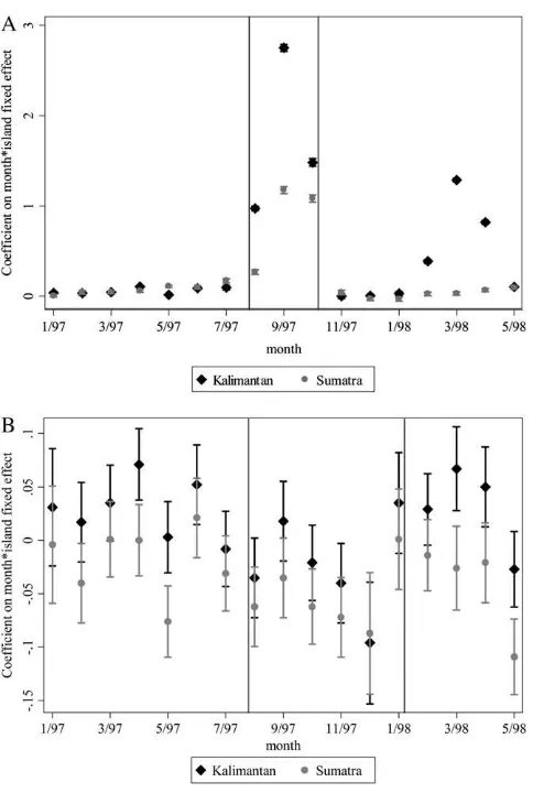
Figure 3 shows the nonparametric relationship between third-trimester exposure and cohort size. The effect of pollution is linear for the most part. There appears to be a somewhat steeper relationship at high levels of pollution, but the nonlinear-ities are statistically insignificant when estimated parametrically with a spline or qua-dratic term.
The next regressions use the pollution level in each of the three months preceding and following birth, rather than aggregated for a quarter. Table 2, Column 6, reports the results using the median pollution level. For prenatal exposure (lags ofSmoke), the ef-fect is strongest two months before the month of birth. For postnatal exposure (leads of Smoke), the effect is strongest immediately after birth, though the estimates are impre-cise. The next two columns repeat the exercise using the month’s mean pollution and the proportion of days that have high pollution. The general pattern of the coefficients for postnatal pollution remains the same, but the pattern for prenatal exposure changes. For the mean pollution level or number of high-smoke days (Columns 7 and 8), expo-sure in the month immediately before the month of birth now has the strongest negative
12. The estimates using high-smoke days imply a 1.0 percent aggregate effect. (The mean of the prenatal high-smoke variable is 0.131 during the 1997-98 episode and 0.006 for the same calendar months a year earlier, and the coefficient in Table 2, Column 4, is20.085.)
13. The government estimates of under-one and under-five mortality rates at this time are 5 percent and 7 percent, respectively. I assume that half of deaths between age one and five occur before age three. 14. The welfare implications of pollution-induced mortality depend on how long individuals otherwise would have lived. One can calculate using the child mortality rate that in the extreme ‘‘havesting’’ scenario, all deaths between ages three and six or seven would have to have been pushed forward to the time of the fires. Moreover, by most standards, the shortening of children’s lives by even a few years is a significant welfare loss.
relationship with cohort size. One interpretation is that at different points during ges-tation, fetuses are more vulnerable to sustained exposure to pollution versus extreme levels of pollution. A more likely interpretation is that there is not enough precision to determine at this level of detail how the timing of exposure affects survival.15Thus, for the rest of the analysis, I focus on the three-month measures of prenatal and post-natal exposure. The results are similar using two-month measures.
B. Effect of Smoke on Mortality versus Alternative Hypotheses
The results in Table 2 suggest that exposure to smoke in utero causes early-life mor-tality. This section considers other possible explanations for the results.
1. Migration
The Census identifies respondents by their subdistrict of current residence, but expo-sure to pollution depends on where one resided during the fires. Migration could be a Figure 3
Kernel Regression of Log Cohort Size on Prenatal Exposure to Pollution
Note: The solid line is the estimated relationship between log cohort size and pollution ( PrenatalS-moke). The dashed lines are the bootstrapped 95 percent confidence interval, with errors clustered within an island-month. The model estimated is a locally weighted nonparametric regression of log cohort size on pollution conditional on year and district fixed effects, following Robinson (1988). Log cohort size has been offset by a constant so that its value is one at an aerosol index of zero.
15. The month-by-month patterns, unlike the results with the three-month measures, are also somewhat sensitive to using a different sample period or a different threshold for high-smoke days.
reason that cohorts with the highest prenatal exposure to pollution are smaller if women in the third trimester of pregnancy were especially likely to migrate away from high-pollution areas, either while pregnant or after giving birth. Fortunately, the Census collects data on the district (though not subdistrict) where an individual was born and where he or she lived five years earlier, which enable one to probe this concern.16
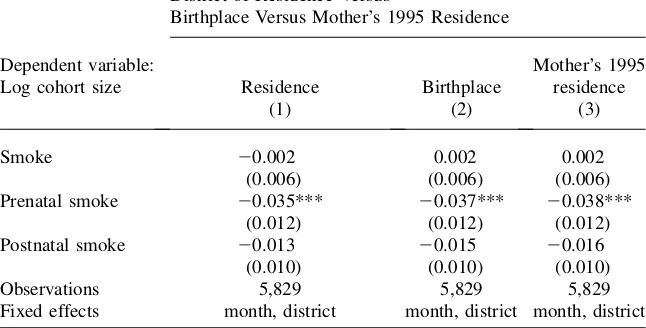
To examine the extent of pollution-induced migration that occursafterbirth, I re-peat the main analysis by district of birth. Cohort size is aggregated to the district level, and the pollution measure for the district is a population-weighted average of the subdistrict measure. The regression is weighted by the district population in the two years prior to the sample period. For comparison, Column 1 of Table 3 presents results by district of residence, and Column 2 presents results by district of birth. The results are nearly identical to each other, as well as to the subdis-trict-level analysis, in terms of both point estimates and precision. Between-district migration after the birth of the infant is not the likely explanation for the relationship between pollution and cohort size.
Pollution-induced migration also may take placebeforethe infant is born. If some women spent most of their third trimester of pregnancy in the hardest-hit areas but migrated away before giving birth, then neither place of residence in 2000 nor place of birth would accurately reflect the fetus’s location during the fires. While the Cen-sus did not ask respondents where they resided in August to October 1997, it did ask where they lived in 1995. As long as people do not migrate across districts repeat-edly, this measure should be a good proxy for where pollution-induced migrants lived at the time of the fires. To test for migration that occurs before birth, I match infants to their mothers as described in the data appendix and repeat the estimate by the district where the mother resided in 1995. The results, shown in Column 3, are unchanged from the earlier estimates. In sum, migration, either before or after birth, does not seem to account for the negative relationship between exposure to pollution and cohort size.17
2. Fertility
The empirical approach interprets decreases inln(CohortSize) as increases in early-life deaths, but there would also be fewer survivors if the number of births decreased. It seems unlikely that conceptions declined nine months before the fires with a spatial pattern matching the pollution, but this concern also can be tested more directly by constructing a measure of predicted births. First, I measure the percentage of women of each age who give birth, using a time period not in the sample (namely, the youn-gest cohorts in the Census, those born in 1999 and 2000). I then apply these birth rates to the demographic composition of each district-month in the sample. This
16. For 9 percent of the sample, district of residence differs from district of birth, for 7 percent it differs from mother’s residence five years earlier, and for 12 percent it differs from one or the other.
17. Within-district migration is unlikely to be driving the results since there is very little within-district variation in pollution, and most of it derives from interpolation so is noisy. In a model with district-month fixed effects, the coefficient forPrenatalSmokeis20.013, smaller than in the main specification
(Table 2, Column 1), and imprecise, suggesting that between-district variation is dominant in the main estimates.
gives a predicted number of births based on demographic shifts. (See the data appen-dix for further details.) Table 4, Column 1, shows the results whenln(PredictedBirths) is included as a control variable. The coefficient of survivors on births is predicted to be slightly less than 1. Because the measure is noisy especially after conditioning on subdistrict and month indicators, the estimate is likely to suffer from attenuation bias. The estimated coefficient on predicted births is less than but statistically indistinguish-able from 1. More importantly, the coefficients on the pollution variindistinguish-ables are essen-tially unchanged with this control variable included. Fluctuations in fertility caused by demographic shifts do not appear to be a confounding factor in the analysis.18
3. Preterm Births
Another concern is that the missing children are not deaths but instead are an artifact of changes in gestation length. Exposure to pollution may have induced preterm de-livery which is often associated with traumatic pregnancies. The reason this mech-anism could conceivably generate the results is that it isprenatalexposure that has a strong negative relationship with cohort size. Consider August 1997, the month the fires started. Pollution levels were high in August, and the value ofPrenatalSmoke for August is low since there was no significant smoke in May, June, or July. In Table 3
Distinguishing Between Mortality and Migration
District of Residence Versus
Birthplace Versus Mother’s 1995 Residence
Dependent variable:
Log cohort size Residence Birthplace
Mother’s 1995 residence
(1) (2) (3)
Smoke 20.002 0.002 0.002
(0.006) (0.006) (0.006)
Prenatal smoke 20.035*** 20.037*** 20.038***
(0.012) (0.012) (0.012)
Postnatal smoke 20.013 20.015 20.016
(0.010) (0.010) (0.010)
Observations 5,829 5,829 5,829
Fixed effects month, district month, district month, district
Note: Each observation is a district-month. Standard errors, in parentheses below the coefficients, allow for clustering at the island-month level. *** indicates p < 0.01; ** indicates p < 0.05, * indicates p < 0.10. Observations are weighted by the number of individuals enumerated in the Census who reside in the district and were born in the year before the sample period.
18. Appendix Table A3 addresses another potential concern about fertility, namely that the seasonality of births or deaths could differ for areas more affected by the pollution, generating a spurious result. The results are robust to restricting the sample to the months with highPrenatalSmokeplus the same calendar months one year earlier.
Table 4
Alternative Hypotheses
Dependent variable: Log cohort size
Control for Predicted
Fertility
Excluding August 1997
SUSENAS and PODES
subsample
Control for Financial Crisis
Excluding Areas with
Fires
Control for Fires
Control for Rainfall
(1) (2) (3) (4) (5) (6) (7)
Smoke 0.001 0.001 0.002 0.002 0.003 0.004 0.001
(0.006) (0.006) (0.006) (0.006) (0.011) (0.006) (0.006)
Prenatal Smoke 20.035*** 20.036*** 20.032*** 20.032*** 20.035** 20.032** 20.032**
(0.012) (0.012) (0.011) (0.011) (0.018) (0.014) 0.013
Postnatal smoke 20.014 20.009 20.012 20.012 0.016 20.005 20.014
(0.009) (0.010) (0.009) (0.009) (0.014) (0.011) (0.009)
Ln(predicted births) 0.875
(0.696)
Financial crisis 20.049
(0.038)
Any fires 20.004
(0.010)
Prenatal any fires 0.007
(0.017)
Postnatal any fires 20.004
(0.014)
Intense fires 20.028*
(0.016)
Prenatal intense fires 20.017
(0.025)
934
The
Journal
of
Human
Postnatal intense fires 20.021 (0.029)
Rainfall 20.023
(0.033)
Observations 67,454 63,703 63,158 63,158 52,646 67,454 67,454
Subdistrict and month FEs? Y Y Y Y Y Y Y
Note: Each observation is a subdistrict-month. Standard errors, in parentheses below the coefficients, allow for clustering at the island-month level. *** indicates p < 0.01; ** indicates p < 0.05, * indicates p < 0.10. Observations are weighted by the number of individuals enumerated in the Census who reside in the subdistrict and were born in the year before the sample period. Predicted Births is constructed using the fertility rate by age and the number of women of different child-bearing ages within a district, as described in the data appendix. The financial crisis variable is standardized to have a mean of 0 and standard deviation of 1 for the sample. Areas without fires are those with fewer than 20 fire-days over the entire period. Any fires is an indicator of any fires and intense fires is an indicator of at least 10 fire-days in the month. The rainfall variable is subdistrict-level rainfall for the 1997 drought months of June to November divided by the 1990–95 average for those calendar months, interacted with a dummy for being in a birth cohort between September 1997 and January 1998.
Jayachandran
September, in contrast,PrenatalSmokeis high since it incorporates the pollution in August. If infants due in September were instead born in August, then births would have shifted from a high-PrenatalSmokemonth to a low-PrenatalSmokemonth, gen-erating a negative relationship betweenPrenatalSmokeand cohort size that is unre-lated to mortality. To test the preterm-birth hypothesis, I repeat the analysis dropping August 1997 from the sample. If the above hypothesis were correct, the coefficient onPrenatalSmokewould become less negative compared to the baseline results. As shown in Table 4, Column 2, this does not occur. The coefficients are nearly iden-tical between the full sample and the subsample, contrary to what one would expect if the pollution had induced preterm births but had not affected infant survival.19
The effect of pollution on cohort size is not due to preterm birthsinstead ofbeing due to fetal and infant deaths. Note, however, that pollution may have caused infant deaths precisely by inducing premature births (which put infants at greater risk of death); that is, preterm delivery is potentially an important channel through which exposure to pollution led to mortality.
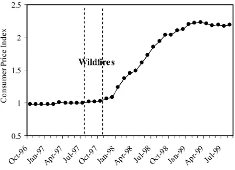
4. Financial Crisis
The Indonesian financial crisis began shortly after the fires, as shown in Figure 4. To verify that the analysis is not attributing to air pollution deaths that were caused by the crisis, a measure of the financial crisis is added to the model. No monthly sub-district-specific data on the crisis were collected, to my knowledge, so I construct a measure of the crisis by interacting a cross-sectional measure, the inverse ratio of median income (consumption) at the height of the crisis in 1999 to median income before the crisis in 1996, and a time-series measure, the consumer price index for food. The regression results can be anticipated by noting that the cross-sectional cor-relation between the crisis measure and pollution in September 1997 (peak of the fires) is 0.03; the spatial patterns of the crisis are not similar to the spatial patterns of pollution. For regressions that use variables from the SUSENAS or PODES sur-veys, a slightly smaller sample of subdistricts is used due to data availability. Table 4, Column 3, shows the regression results for the baseline model and confirms that the subsample is similar to the full sample, with a coefficient onPrenatalSmoke of
20.032. Column 4 then shows the results when the crisis measure for the month of birth is included as a control variable. The estimated effect of PrenatalSmoke remains 20.032. The crisis measure has been normalized to have a mean of zero and standard deviation of one for the sample, so the coefficient implies that a one standard deviation increase in the crisis is associated with a 4.9 percent smaller co-hort, though the coefficient is statistically insignificant (and moreover could be due to migration rather than mortality).20;21
19. Appendix Table 3 restricts or expands the sample to other time periods, and the results are robust to this change. One noteworthy finding is that the estimated effect ofPrenatalSmokeis smaller when the window extends more than eight months after the fires, suggesting that the fires may have reduced fertility. 20. Since the crisis accelerated a few months after the fires, I also estimated models that control for the crisis measure for the three months following the month of birth. This generates more variation in the crisis measure during the period of interest. The estimated effect ofPrenatalSmokeis unchanged.
21. Rukumnuaykit (2003) finds a 3 percent increase in infant mortality in 1997-98 in the Indonesia Family Life Survey, which is interpreted as due to the financial crisis, drought and smoke.
5. Effect of Pollution versus Effect of Fires or Drought
Another interpretation of the results is that they represent reduced-form effects of the fires rather than effects of specifically air pollution. The regressor is the pol-lution level, but the smoke affected places nearby the sites of fires, and the fires could have caused mortality through income effects, degraded food supply, and other channels. To separate the effect of pollution from other effects of the fires, I use data on where the fires occurred. I calculate the number of fire-days occur-ring in or near a subdistrict based on satellite data on ‘‘hot spot’’ locations and durations.Firedaysis the duration of each fire summed over all fires within 50 km of the subdistrict center. First, I examine the effects of pollution in areas that did not experience extensive fires. In essence, the identification comes from fires in neighboring areas and the direction that the winds blew the pollution. In Table 4, Column 5, the sample is restricted to subdistricts where fewer than 20 fire-days occurred over the sample period, which eliminates 22 percent of subdistricts, pre-dominantly in Kalimantan and Sumatra.22 The coefficient onPrenatalSmoke on log cohort size remains20.035 for these areas that experienced only the pollution from the fires. Next, I include measures of fire prevalence as regressors. The fire-days variable is highly skewed, so I use two indicator variables, one for whether there were any fire-days in the subdistrict-month (sample mean of 0.16) and a sec-ond for whether there were intense fires, defined as at least ten fire-days during the month (sample mean of 0.03). In Column 6, the fires variable and intense fires Figure 4
Timing of the Fires and the Financial Crisis
22. Because of measurement error in the hotspot data, eliminating any subdistrict with at least one fire-day would eliminate more than two-thirds of subdistricts, which is inconsistent with the actual geographic ex-tent of the fires. Fewer than 22 percent of subdistricts were probably affected, so the results shown are con-servative. They are similar if other thresholds are chosen.
variable in the month of birth, averaged over the three months before birth (pre-natal exposure), and averaged over the three months after birth (post(pre-natal expo-sure) are included as regressors. The effect ofPrenatalSmoke is20.032, nearly identical to earlier estimates, which supports the interpretation that air pollution is the cause of the increase in early-life mortality. There is also some evidence that intense fires in the month of birth are associated with a decrease in cohort size, suggesting that fires may have an additional effect on survival (or migration) through channels besides pollution, but the effect size is relatively small. The co-efficient of20.028 implies that intense fires are associated with a 0.25 percent de-crease in cohort size.
Another hypothesis is that the effects are due to the drought. There was below-normal rainfall throughout Indonesia in 1997, not just in areas affected by pollu-tion; given that month fixed effects are included, drought seems unlikely to be driving the results. Nevertheless, I test directly for effects of the drought and in a way that stacks the cards in favor of finding that the drought is driving the results. Monthly rainfall for the subdistrict is measured relative to the 1990–95 av-erage for that calendar month, and I construct the subdistrict-level mean for the months of June to November 1997, when the drought occurred. The mean of this variable is 0.48. I then control for this measure of rainfall interacted with an indi-cator for being in a birth cohort between September 1997 and January 1998. In other words, the drought is assumed to affect specifically the cohorts that I find are harmed by the pollution. As shown in Table 4, Column 7, the coefficients for the pollution variables are essentially unaffected when rainfall is included as a control. The coefficient for rainfall is statistically insignificant and small. The results are similar controlling for contemporaneous rainfall in the month or rainfall with a one to nine-month lag. One might worry that drought reduces fertility, but the drought began in June, and the affected cohorts were conceived by April. Moreover, when rainfall nine months prior to birth is added as a control variable, again, rainfall has a small and insignificant effect on cohort size, and the effect of prenatal pollution is unchanged. The changes in cohort size do not seem to be due to rainfall shortages.
C. Effects by Gender and Income
1. Effects by Gender
exposure to pollution or to seek medical treatment for his respiratory infection, for example, then one would expect the effects of postnatal pollution to be stronger for girls. However, these interpretations should be treated with caution since the gen-der differences are not statistically significant.
2. Effects by Income
The next estimates test whether the effects of pollution are more pronounced in poorer places. This type of heterogeneity could arise if the poor effectively are ex-posed to more pollution, for example, because they spend more time outdoors do-ing strenuous work or are less likely to evacuate the area. It could also arise if the same amount of effective pollution leads to bigger health effects for the poor, for example, because they have lower baseline health, making them more sensitive to pollution, or have less access to healthcare to treat the health problems caused by the pollution.
Column 2 of Table 5 uses food consumption as a proxy for income to examine this hypothesis, interacting the pollution measures with a dummy variable for whether the district’s median log consumption in 1996 is above the 50th percen-tile among all subdistricts. All three of Smoke, PrenatalSmoke, and Postnatal-Smoke are associated with smaller cohorts for the bottom half of the consumption distribution, and the interaction terms for the top half of the distri-bution are large and positive. The weighted average of the coefficients for the bottom and top halves of the distribution would be more negative than the aver-age effect found earlier, however. The reason is that month effects vary with in-come. As has been documented in the demography literature, seasonality in fertility tends to be stronger and qualitatively different in poorer areas (Lam and Miron 1991). Thus, Column 3 includes separate month fixed effects for the top and bottom halves of the consumption distribution. The results are qualita-tively similar to those in Column 2. The effect of prenatal exposure is large and negative when consumption is below the median. In these areas, postnatal ex-posure is also statistically significant, with an effect size about 60 percent that of prenatal exposure. Each of the interaction coefficients for districts with above median consumption is positive, and in the case of PrenatalSmoke, significant at the 1 percent level. The effect of a one unit change in PrenatalSmoke is
20.06 for the top half of the distribution and 20.13, or over twice as large, for the bottom half. Average log consumption is 0.4 log points larger in the top half of the distribution compared to the bottom half, so another way to view the results is that when consumption increases by 50 percent (e0.4), the effect size decreases by 50 percent.
The dependence of seasonal patterns on income suggests that including separate month effects for the two halves of the consumption distribution might be the pre-ferred specification even for estimating the average effect. In addition, for the rea-sons explained by Deaton (1995), given the heterogeneous effects, the average effect should be calculated by separately estimating the effect by consumption level and then averaging. This amounts to averaging the coefficients in Column 3, weighted by the population in each half of the consumption distribution. As shown in Column 4, the average effect for prenatal smoke is then 20.090 and
Table 5
Effects by Gender and Income
By gender By income (log consumption) of the district
Top quartile
3rd quartile
2nd quartile
Bottom quartile Dependent variable:
Log cohort size
(1) (2) (3) (4) (5)
Smoke 20.008 20.060*** 20.024 20.013 20.004 20.011 20.028 0.002
(0.007) (0.021) (0.016) (0.017) (0.009) (0.010) (0.024) (0.045)
Prenatal smoke 20.030** 20.158*** 20.129*** 20.090*** 20.058*** 20.076*** 20.094** 20.121**
(0.012) (0.037) (0.028) (0.015) (0.018) (0.017) (0.047) (0.061)
Postnatal smoke 20.019* 20.158*** 20.047* 20.035** 20.025 20.040*** 20.046 0.009
(0.010) (0.027) (0.024) (0.019) (0.016) (0.014) (0.032) (0.052)
Male 0.014***
(0.003)
Smoke * male 0.016***
(0.005)
Prenatal smoke * male 20.009
(0.007)
Postnatal smoke * male 0.010
(0.006) Smoke * high
consumption
0.066*** (0.021)
0.017 (0.014)
Prenatal smoke * high consumption
0.127*** (0.038)
0.072*** (0.027)
940
The
Journal
of
Human
Postnatal smoke * high consumption
0.161*** (0.026)
0.017 (0.014)
Observations 134,734 63,158 63,158 63,158 63,158
Fixed effects included
subdistrict, month
subdistrict, month
subdistrict, month * high cons.
subdistrict, month * high cons.
subdistrict, month*quartile of log consumption
Note: Each observation is a subdistrict-month. Standard errors, in parentheses below the coefficients, allow for clustering at the island-month level. *** indicates p < 0.01; ** indicates p < 0.05, * indicates p < 0.10. High consum. is an indicator that equals 1 if the district’s median log food consumption is above the sample median. Obser-vations are weighted by the number of individuals enumerated in the Census who reside in the subdistrict and were born in the year before the sample period. Column 4 reports the average of the coefficients in Column 3, weighted by the population in each half of the consumption distribution; the standard error and the joint significance of the linear combination of coefficients is shown.
Jayachandran
the coefficient for postnatal smoke is20.035, both considerably larger than seen earlier in Table 2.
Next, I further break down the income distribution into quartiles (and include month-quartile fixed effects). Column 5 shows the separate coefficients by quar-tile, estimated as one regression. The point estimate on PrenatalSmokebecomes more negative moving from higher to lower quartiles. The results are not very precise, though, and the PrenatalSmoke coefficients for different quartiles are not statistically distinguishable from one another. The coefficients for the other smoke variables are also imprecise, especially for the bottom two quartiles, and the point estimates do not monotonically decline with consumption. Above- ver-sus below-median consumption, as opposed to a linear interaction term, is there-fore used below to parsimoniously characterize the heterogeneous effects by income.
3. Effects by Urbanization, Wood-Stove Use, Healthcare, and Mother’s Education
This subsection tests some hypotheses about why there is an income gradient in the health effects of pollution. The tests are merely suggestive because the measures used could be correlated with omitted variables and data are available to test only a limited number of hypotheses.
One possibility is that urban areas experience smaller effects from the fires than rural areas, generating the heterogeneity by income. Urbanization would only be a proximate cause, but one might think that in urban areas, housing stock is less permeable, healthcare is better, there is less outdoor work, or there are more effective public advisories urging people to stay indoors, for example. On the other hand, pollution from the fires may have been particularly noxious in cities where it mixed with industrial pollution from cars and factories. Column 1 of Table 6 interacts the pollution measures with the proportion of the subdistrict population that lives in urban localities (based on those born in the year before the sample period). Only the coefficients for PrenatalSmoke and its interaction terms are reported, but Smoke,PostnatalSmoke, and their interactions are also included in the regres-sions. The effects of pollution do not vary by urbanization level, suggesting that the effects described above may have offset each other. In unreported results, I also find that children whose mothers work in agriculture do not experience larger effects.
Table 6
Effects By Urbanization, Wood Fuel Use, and Healthcare Sector
Dependent variable: log cohort size (1) (2) (3) (4) (5)
Prenatal smoke 20.121*** 0.015 20.115*** 20.113*** 20.007
(0.028) (0.032) (0.027) (0.028) (0.025)
Prenatal smoke * urbanization 20.013
(0.013)
Prenatal smoke * wood fuel use 20.155*** 20.120***
(0.036) (0.026)
Prenatal smoke * maternity clinic 0.030*** 0.011**
(0.009) (0.005)
Prenatal smoke * doctors 0.048*** 0.016
(0.015) (0.013)
Prenatal smoke * high consumption
0.071*** 0.048* 0.058** 0.052** 0.044*
(0.027) (0.025) (0.025) (0.025) (0.025)
Observations 63,158 63,158 63,158 63,158 63,158
Subdistrict and month FEs? Y Y Y Y Y
Note: Each observation is a subdistrict-month. Standard errors, in parentheses below the coefficients, allow for clustering at the island-month level. *** indicates p < 0.01; ** indicates p < 0.05, * indicates p < 0.10. All regressions also include Smoke and Postnatal Smoke and their interactions with the relevant variables for each column. Urbanization is the proportion of the population in urban localities and is based on 1994 to 1996 birth cohorts. Wood fuel use is an approximate measure of the proportion of people in the subdistrict who cook with wood fuel rather than kerosene and gas. Health variables are normalized to be mean zero, standard deviation one for the sample. High consumption is an indicator that equals one if the district’s median log food consumption is above the sample median. Observations are weighted by the number of individuals enumerated in the Census who reside in the subdistrict and were born in the year before the sample period.
Jayachandran