T H E J O U R N A L O F H U M A N R E S O U R C E S • 46 • 3
Which Reference Groups Matter?
Eiji Mangyo
Albert Park
A B S T R A C T
We examine the extent to which self-reported health and psychosocial health are affected by relative economic status in China, for the first time examining the importance of reference groups not defined by geographic location or demographic characteristics. We propose a methodology to ad-dress potential bias from subjective reporting biases and control for unob-served community characteristics. Analyzing a nationally representative data set from China, our findings support the relative deprivation hypothe-sis and suggest that relatives and classmates are salient reference groups for urban residents and neighbors are important for rural residents.
I. Introduction
A growing literature provides evidence that individual health and subjective well-being are influenced by relative economic status (Eibner and Evans 2005; Ferrer-i-Carbonell 2005; Luttmer 2005). According to the relative deprivation hypothesis, feeling less well off than others creates unhappiness and stress, which leads to worse health, contributing to a negative relationship between income in-equality and health (Wilkinson 1996). The theory assumes that utility is a function not only of own consumption, but also of the consumption level of others in one’s social reference groups. The relative deprivation hypothesis can rationalize empirical evidence that the health gradient exists over the whole spectrum of socioeconomic status in rich countries rather than disappearing above an income threshold (Marmot et al. 1991; Davey Smith, Shipley, and Rose 1990; Der et al. 1999). It is also consistent with the strong positive correlation between income and subjective
well-Eiji Mangyo is an associate professor of economics at International University of Japan. Albert Park is a Reader in Economics at the University of Oxford. The authors acknowledge primary funding support for the China Inequality and Distributive Justice survey project from the Smith Richardson Foundation, with supplementary funding provided by Harvard’s Weatherhead Center for International Affairs, the University of California at Irvine, and Peking University. They also thank two anonymous referees for very helpful comments. The data used in this article can be obtained beginning January 2012 through December 2015 from Albert Park ⬍albert.park@economics.ox.ac.uk⬎; Manor Road Building, Manor Road, Oxford OX1 3UQ, UK.
[Submitted December 2007; accepted August 2010]
being found in cross-sectional data but the failure of average happiness to increase as societies become richer (Easterlin 1995). Health and subjective well-being are likely to be strongly connected given that medical studies find a large impact of stress on the incidence and progression of many illnesses (Lovallo 1997; Sapolsky 1998).
A major challenge in studying the relative deprivation hypothesis is defining ap-propriate reference groups to which individuals compare themselves (Eibner and Evans 2005). Because of the limited content of most social surveys, previous em-pirical studies all have defined reference groups based on geographic location or demographic characteristics such as age, gender, or ethnicity. However, other social reference groups with which individuals have frequent social contact may be much more salient, for example relatives, coworkers, and former classmates. Even for geographic reference groups, previous research has not systematically studied which level of geographic aggregation has the greatest influence on individual health and sense of well-being. In particular, neighbors living in close proximity may be a particularly important reference group. It is also likely the relative importance of different types of social reference groups may differ across individuals.
In this paper, we empirically investigate for the first time the impact on health of relative deprivation defined with respect to multiple social and geographic reference groups. We analyze data from a unique national survey in China that includes ques-tions about respondents’ subjective assessments of how their living standards com-pare to different geographic and nongeographic reference groups. China is a par-ticularly interesting case because it is not only the world’s most populous country but also a nation that has witnessed a very rapid increase in income inequality during its transition from a socialist planned economy to a market-based system. China’s gini coefficient increased from 0.309 in 1981 to 0.453 in 2003 (World Bank, 2009). This paper also makes a methodological contribution by showing how subjective questions about relative economic status can be used to investigate the relative dep-rivation hypothesis without being undermined by subjective reporting biases. Such biases arise because individual outlooks (optimism or pessimism) may influence both subjective welfare assessments and self-reports of health status. We address this problem by directly estimating the magnitude of such biases and controlling for them in our econometric analysis. In addition, we control for unobserved regional characteristics affecting health by including regional fixed effects, which is not pos-sible in most other studies in this literature that use regional income measures to test the relative deprivation hypothesis. The lack of adequate controls for omitted regional characteristics may be one reason why previous studies find mixed results on the effect of relative deprivation on health.
The rest of the paper is organized as follows. The next section reviews previous studies on the effects of relative income on health. Data and descriptive statistics are presented in Section III, Section IV describes the research methodology, Section V presents the results, and Section VI concludes.
II. Relative Deprivation and Health
influ-ence an individual’s sense of well-being or happiness. Studies have found a link between stress caused by economic hardship and health-related behaviors such as smoking, heavy alcohol use, and less healthy diet (Conway et al. 1981; Gorman 1988; Horwitz and Davies 1994; Jensen and Richter 2004; Kristenson et al. 1999). Second, other social and political mechanisms also may link relative economic status and individual health. The relatively poor may lack social cohesion with others; the quality of social relationships has been found to be associated with unhealthy be-haviors and poorer health (House, Landis, and Umberson 1999). Third, the relative poor may have relatively less access to healthcare or other services if access is rationed or subject to political influence. Although it is difficult to distinguish em-pirically between the first two explanations, the third is less likely to strongly affect psychosocial health than the first two.
This study extends the work of previous authors who have examined the empirical relationship between relative deprivation and health outcomes and health behaviors. Eibner and Evans (2005) analyze U.S. microdata and find that relative deprivation with respect to individuals with similar demographic characteristics reduces self-reported health status, increases mortality, and increases risky health behaviors (smoking, obesity, less exercise). Other research based on survey data also has found an empirical link between relative deprivation and both mortality and suicide (Eibner and Evans 2005; Miller and Paxson 2006; Daly, Wilson, and Johnson 2007), but not all studies find a mortality effect (Gerdtham and Johannesson 2004). Even experi-mental research on primates has found that low social status leads to higher choles-terol, increased atherosclerosis, obesity, and depression (Shively and Clarkson 1999; Shively, Laber-Laird, and Anton 1999; Sapolsky, Alberts, and Altmann 1999). A number of studies also have found a close relationship between relative economic status and subjective well-being (Luttmer, 2005; Ferrer-i-Carbonell 2005; McBride 2001). As noted earlier, all of these studies examine reference groups defined by geographic and demographic characteristics and are unable to fully rule out bias from omitted regional characteristics.
As first motivated by Wilkinson (1996), the relative deprivation hypothesis could explain a negative relationship between income inequality and average health of the population. However, it is important to point out that the inequality-health relation-ship could also be influenced by factors unrelated to the relative deprivation hy-pothesis, such as concavity of the income-health relationship and less provision of public goods (for example, health services) in communities with greater income inequality due to political economy reasons, etc.1In this paper, we restrict attention
to testing the impact of relative economic status on individual health, and do not directly address the recent literature relating income inequality to aggregate health (Deaton and Paxson 2001; Deaton 2002 and 2003; Kawachi and Kennedy 1997; Kennedy et al. 1998; Mellor and Milyo 2002).
III. Data
Our data come from the China Inequality and Distributive Justice survey project conducted in the fall of 2004, which collected data on a nationally representative sample of 3,267 Chinese adults between the ages of 18 and 70 living in 23 of China’s 31 provinces and in 65 counties and 85 townships.2Respondents were selected using spatial probability sampling methods. Important for our pur-poses, the survey included questions asking the respondents to rate their living stan-dards in comparison with multiple reference groups. Specifically, the survey asked, “Compared with the average living standard of [your relatives, classmates with the same level of schooling as you, your coworkers, your neighbors, others in the same county or city, others in the same province, others living in China], do you feel your living standard is much better, a little better, about the same, a little worse, or much worse?” These questions are coded from one to five, with five being “much better”. We use two health measures. The first is self-reported health status (1⳱very poor, 2⳱poor, 3⳱average, 4⳱good, 5⳱very good). The second is an index measure of
psychosocial health based on eight questions: “Below are some descriptions of peo-ple’s life conditions. In the past week, did you experience these conditions: often, sometimes, rarely, or never? (a) I worry about some small things. (b) I have no appetite for food. (c) I cannot focus my attention while doing things. (d) I feel my life is a failure. (e) The quality of my sleep is poor. (f) I feel fortunate. (g) I feel alone. (h) I feel my life is very happy.” The answers to each question are coded from 1 to 4, with 4 being better psychosocial health. To calculate an index of psy-chosocial health, the answers to each question are normalized to be standard devi-ations from the mean, and the index is the mean of the normalized scores for the eight questions. Psychosocial health is a particularly appropriate measurement for examining the relative deprivation hypothesis, which posits that health is affected largely through dissatisfaction or stress caused by relative economic status.
The eight questions for measuring psychosocial health come from the CES-D scale (Center for Epidemiologic Studies Depression scale), originally proposed by Radloff (1977). The validity of the scale as a depression measure is confirmed by numerous studies including Knight et al. (1997), Lin (1989), Zhang et al. (2002), and Li and Hicks (2010), the latter three of which validate the CES-D in Chinese cultural set-tings.
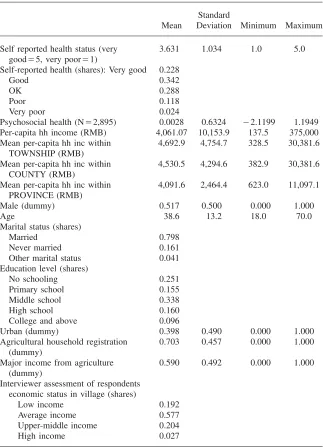
The survey also collected information about individual demographic characteris-tics and household income. Table 1 shows descriptive statischaracteris-tics for the main ables. The sample size is 2,891 individuals with complete information for all vari-ables used in the regression analysis. The self-reported health status of the great majority of individuals is average or better (85.8 percent). With regard to psycho-social health, a significant share of respondents report sometimes or often having negative experiences such as having no appetite (33.2 percent), being unable to focus
Table 1
Self-reported health (shares): Very good 0.228
Good 0.342
OK 0.288
Poor 0.118
Very poor 0.024
Psychosocial health (N⳱2,895) 0.0028 0.6324 ⳮ2.1199 1.1949
Per-capita hh income (RMB) 4,061.07 10,153.9 137.5 375,000 Mean per-capita hh inc within
Male (dummy) 0.517 0.500 0.000 1.000
Age 38.6 13.2 18.0 70.0
Urban (dummy) 0.398 0.490 0.000 1.000
Table 1(continued)
Mean
Standard
Deviation Minimum Maximum
Interviewer assessment of respondents housing (shares):
Poor 0.121
Middle 0.697
High 0.182
Own assets (dummies): Motorcycle 0.352 0.478 0.000 1.000
Car 0.046 0.209 0.000 1.000
Refrigerator 0.343 0.475 0.000 1.000
Color TV 0.779 0.415 0.000 1.000
Computer 0.112 0.316 0.000 1.000
Telephone/cellphone 0.637 0.481 0.000 1.000
Washing machine 0.458 0.498 0.000 1.000
Household size 4.1 1.5 1.0 14.0
attention (31.0 percent), feeling their life is a failure (23.8 percent), having poor quality sleep (39.0 percent), and feeling alone (26.3 percent). For a full description of answers to all questions used in the index, see Appendix Table A1.
Next we describe respondents’ perceptions of how their own living standards compare to seven reference groups: three nongeographical (relatives, classmates, and coworkers), and four geographical (neighbors, county or city, province, and nation). Full results are presented in Appendix Table A2. For the nongeographical reference groups, the most common response is that living standards are similar to others in the reference group, but there is substantial variation in these rankings.3 For geo-graphic reference groups, an interesting pattern emerges in which the greater the geographic scope of the reference group, the more likely that individuals report being less well off than the reference group. Thus, a majority of respondents feel that they have lower living standards than the typical person in China.
The survey asks respondents to report their household income for the entire year of 2003. Of the total 3,267 sample individuals, 2,907 report income: 2,517 individ-uals (77 percent) report a precise value for their household income and 390 indi-viduals (12 percent) report a range for their household income in which case income is set equal to the range mid-point.4Less than one percent of respondents (25) report zero household income; in order to be able to calculate log per capita income, for
3. Some questions have high percentages of missing values because the questions are not applicable, for instance, if the respondent did not attend school or has little or no contact with former classmates, or the person is not working.
respondents with income in the lowest one percent, we set per capita income equal to per capita income at the first percentile.5
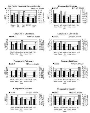
Next, we show how self-reported health and psychosocial health are correlated with how individuals rate themselves with respect to different reference groups. We calculate the mean health of individuals who report different relative economic status and plot the results (Figure 1). We also plot the relationship between health and household income level. For self-reported health status, there are strong associations between health and the perception of own living standards in comparison with others in each of the seven reference groups. We also see a strong correlation between self-reported health and per-capita income quintile. Turning to the psychosocial health index, the associations are less evident in general, but psychosocial health scores are clearly low when individuals consider that their living standards are somewhat or much worse than that of others.
IV. Empirical Methodology
According to the relative deprivation hypothesis, controlling for a person’s own income, people feel more deprived and thus have poorer health when others in a reference group have higher incomes. A frequently used objective mea-sure of relative income is the mean living standards of others living in the same geographic area (sometimes also broken down by demographic group). In this study, we use both township-level and province-level mean log income per capita as ob-jective relative deprivation measures in addition to the seven subob-jective relative-income measures described above.6Township may denote a rural town (xiang or zhen) or an urban subdistricts (jiedao), which share the same administrative level in China.
The basic estimating equation is as follows:
H⳱ⳭYⳭRⳭXⳭTOWNⳭε,
(1) i 0 1 i 2 i 3 i 4 t i
where the subscripts iand trepresent individuals and towns (or city subdistricts), is self-reported health status or psychosocial health, is log per-capita household
Hi Yi
income,Riis a measure of relative income,Xiis a vector of demographic variables including an indicator variable for whether the place of residence is in an urban or rural community,TOWNtis a vector of dummy variables for each townshipt,εiis an error term, and thek are coefficients to be estimated.
First, we estimate Equation 1 using OLS, objective relative-income measures, and no regional fixed effects, which is similar to the specification adopted in many previous studies. We cluster standard errors at the township level to take into account potential correlations of health across individuals living in the same community. The relative deprivation hypothesis predicts that mean regional income levels should have
5. Fifty-three sample individuals report per-capita household income below the cutoff which is 137.5 RMB. Results are not sensitive to the specific cutoff line chosen.
Figure 1
Self-Reported Health and Psychosocial Health, by Relative-income Status with Respect to Different Reference Groups
Next, we estimate Equation 1 using OLS with subjective measures of relative income, initially excluding regional fixed effects as before. We estimate the impact of each subjective relative-income measure one by one (relatives, classmates, co-workers, neighbors, county, and province).
As noted earlier, one advantage of using subjective measures of relative income with respect to nongeographic reference groups is that we can include regional fixed effects since the subjective measures vary at the individual level.7The lowest level
of clustered sampling in our data set is the township level, so inclusion of township fixed effects maximizes our ability to control for unobserved geographic character-istics. Although it is possible that regional differences at lower levels of spatial aggregation (rural village or urban neighborhood) could still bias our estimates, in China townships are the lowest administrative level of government and are the site of state-run medical clinics, bank branches, and other important local institutions. Therefore, township fixed effects should effectively control for key unobserved dif-ferences in policy, quality of medical services, and other geographic and institutional factors. When we include township fixed effects we are unable to include objective measures of relative-income status with respect to geographic reference groups ag-gregated to the township level or above. We cluster standard errors at the township level for the same reason as before.
We are concerned about bias due to unobserved individual outlooks, because our measures of health and relative income are both subjective. For example, people who like to complain or are pessimistic may report poorer self-reported health as well as lower relative-income status. In this section, we show how one can directly estimate individual outlook bias and explicitly control for it in estimation. The es-sential idea is to define the difference between one’s subjective rating of relative living standards within one’s county of residence and one’s actual income position within the county as a measure of optimism or pessimism. We focus on county comparisons because the county is the smallest geographic area with sufficient ob-servations for both objective and subjective income measures.
To see more clearly how this is implemented, consider the following reduced-form function for the determinants of health:
H⳱H(Y,R ,u,o,u).
(2) i iJ i i J
Here, Yiis true household income,RiJis subjective relative income of individuali with respect to some reference groupJ,uiis individual and household unobservables affecting health that are independent of attitudinal biases that affect reporting of relative incomes, oi is the unobserved outlook of individuals that can affect both health and perceptions of relative income, anduJis unobserved group characteristics that affect health.
We posit that RiJis a function of household income, mean community income, and outlook bias:
R ⳱R(Y,Y,o).
(3) iJ i J i
We recognize thatYiandYJ may both be measured with error:
˜ ˜
Y⳱YⳭe and Y⳱YⳭe.
(4) i i i J J J
Thus, Y˜i and Y˜J are noisy measures of true household income and group mean income.
We propose the following approach to estimating Equation 2 to reduce likely biases. We start by first estimating the determinants of the relative-income measure with respect to a reference group for which we have multiple observations within each group (that is, counties). Assuming that relative income can be expressed as a linear function of its elements, we can estimate the following equation:
R ˜
R ⳱␣Ⳮ␣YⳭ␥Ⳮε .
(5) iJ 0 1 i J i
The county fixed effect ␥J absorbs the effect of true group mean income (YJ). Given Equations 3 and 4, if we estimate Equation 5 using OLS the error term will have two components, . Since the error term containsei, it is clearly
R
εi⳱ⳮ␣1eiⳭoi
correlated with ˜Yi, leading to biased estimates due to measurement error. However, using instrumental variables, it is possible to estimate ␣1 consistently so that the error term will consist only of omitted outlook bias. In estimating Equation 5, we instrument log income per capita using the two assessments of the household’s stan-dard of living relative to others in the community made by the survey enumerator who interviewed the household, which are plausibly independent of income mea-surement error and outlook bias.8We use the residual from this 2SLS estimation as
our estimate of outlook bias (oˆ).9 This estimate is unbiased but measures actual
i
outlook bias with noise. If we assume that outlook bias affects all self-reported relative-income measures similarly, these residuals can be used to control for outlook bias when estimating the effects of subjective relative income with respect to ref-erence groups for which multiple observations are not available.
We now are ready to estimate the following equation for the determinants of health outcomes:
H ˜
H⳱ⳭYⳭR ⳭoˆⳭε .
(6) i 0 1 i 2 iJ 3 i i
Given the health production function described in Equation 2, in Equation 6 the error term includesuiwhich is independent by assumption, anduJ. We will be unable to fully isolate the effect of relative income on health, because group mean income (or unobservables correlated with group mean income) can have independent effects on health. However, as a general rule, most of the likely effects of greater group
8. The two specific questions are the following: (1) “From your impression of the respondent’s household, please evaluate whether in the local area the household would be considered a low income household, average income household, upper middle-income household, or high income household?”; and (2) “How does the respondent’s home compare to the average home in the area: below average, average, or above average?”
mean income on health should be positive. For example, having more affluent rela-tives, classmates, or coworkers could improve one’s health through remittances, in-formation about health, or help in accessing better quality healthcare services. In contrast, the relative deprivation hypothesis predicts that greater group mean welfare (or lower relative income) reduces a person’s own health. This suggests that a posi-tive effect of relaposi-tive income on health should be viewed as strong evidence in favor of the relative deprivation hypothesis. Differences in the effect of relative income with respect to different reference groups could reflect differences in both the impact of relative deprivation on health and other independent effects of group mean welfare on health.
In Equation 6, income ˜Yiincludes measurement error which could lead to atten-uation bias. We can check the extent to which this is important by instrumenting for income.10
If self-reports of health status reflect comparisons individuals make between their own health and others in their social reference group, then measured impacts of relative income on health could influence how respondents report their health rather than their actual health.11Our measure of psychosocial health could be considered
more objective and less subject to such bias, given that it is based on questions which ask about the frequency of specific experiences rather than for a general assessment. To address this concern, ideally one would test how relative income affects highly objective measures of health status, such as physical health exam results or incidence of specific diseases or health conditions; unfortunately, such data are not available in the survey.
V. Results
We first report results of OLS estimation using objective relative-income measures with respect to geographic reference groups. Columns 1 and 2 of Table 2 present the results for self-reported health status and psychosocial health, respectively. For both measures, higher own income is significantly associated with better health. Based on the point estimates a doubling of income would increase self-reported health status by 0.113 ranks (0.109 standard deviations) and improve psychosocial health by 0.098 standard deviations. Township mean log per-capita household income negatively affects both health measures after controlling for own income, consistent with the relative deprivation hypothesis. However, the coefficient
10. The instruments are a set of seven wealth indicator variables that reflect whether the household owns the following assets: motorcycle, car, refrigerator, color TV, computer, phone, and washing machine. While such instruments deal with the measurement error problem, they will not convincingly deal with possible simultaneity bias due to the positive effect of health on income if such effects are persistent and so also determine household assets. Simultaneity bias would likely lead to upward bias in the coefficient on income and downward bias on the coefficient on relative income.
Table 2
OLS with Objective Measures of Relative Income
(1) (2) (3) (4)
Dependent variable SRHS Psych. SRHS Psych.
Log per-capita hh income 0.113** 0.098** 0.095** 0.084**
(0.043) (0.039) (0.039) (0.034)
Male (dummy) 0.156*** 0.158*** 0.163*** 0.164***
(0.057) (0.050) (0.054) (0.048)
Age/10 ⳮ0.284* ⳮ0.191* ⳮ0.298* ⳮ0.202*
(0.156) (0.104) (0.160) (0.106)
(Age/10)2 0.012 0.018* 0.013 0.019*
(0.017) (0.011) (0.018) (0.011)
Degree⳱⳱primary (dummy) 0.239** 0.135** 0.226** 0.138**
(0.094) (0.055) (0.091) (0.056)
Degree⳱⳱tertiary (dummy) 0.309 0.031 0.280 ⳮ0.000
(0.204) (0.103) (0.194) (0.095)
Degree⳱⳱no response
(dummy)
ⳮ0.339 0.014 ⳮ0.372 0.012
(0.305) (0.091) (0.308) (0.102)
Urban resident (dummy) ⳮ0.109 ⳮ0.093 ⳮ0.136 ⳮ0.123*
(0.096) (0.075) (0.087) (0.069)
AdjustedRSquare 0.152 0.064 0.151 0.064
Notes:
(1) Omitted or reference categories are married for marital status and less than primary schooling for education.
(2) Standard errors are clustered by township.
on township mean income is statistically significant at conventional levels only for psychosocial health (Column 2). In fact, for psychosocial health, the magnitude of the negative effect of mean township income is even greater than the positive effect of own income.
For other demographic variables, the coefficient estimates are mostly as expected. Males report themselves to be healthier than females. As people age, their health becomes worse at a decreasing rate (the coefficient on the age squared term is positive and statistically significant at the 10 percent level for psychosocial health). Psychosocial health of unmarried persons is significantly worse than that of married persons, but self-reported health status is similar. Education has a nonlinear rela-tionship with health. Health increases with educational attainment through middle school, but with more education beyond middle school it fails to increase or even falls. Residing in urban areas is associated with poorer health after controlling for other covariates, but the effect is not statistically significant at conventional levels.12
We also investigate whether provincial income per capita predicts health out-comes. Results are presented in Columns 3 and 4 of Table 2. Provincial income per capita is negatively associated with psychosocial health but positively associated with self-reported health; however, the associations are not statistically significant. This suggests that others in the township are a more salient comparison group than others in the province, or that unobserved provincial differences associated with mean income have more positive impacts on health than unobserved township dif-ferences.
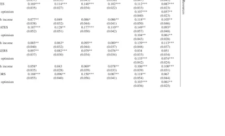
Next, we turn to the results using the subjective relative-income measures. Table 3 reports the coefficients when we use subjective assessments of relative income with respect to different reference groups.13In each of these regressions, we include the same covariates as before, but because they do not differ substantially from the patterns found in Table 2, we do not report their coefficients in this or subsequent tables. As noted earlier, some subjective assessments have a nontrivial number of missing observations; to deal with this, we add a dummy variable for whether the relative-income measure is missing and assign a zero to the measure of relative income.14
We start with the exact same specification as in Table 2, but using subjective relative-income measures rather than objective ones. Results are reported in Columns 1 and 2 of Table 3. In general, the coefficient on the household’s own income is positive and statistically significant, but somewhat smaller in magnitude than when objective relative-income measures are used. This is to be expected, since the rela-tive-income measure is the difference between own income and that of others rather than the mean income of others. This means that the coefficient on relative income captures part of the effect of own income and that the coefficient on own income
12. The control variables also include a dummy for bottom-coding of per-capita household income (set equal to the one percent cutoff value).
13. We do not examine subjective comparisons with China as a whole because this would lead to a fallacy of composition in that since the sample is a national one. For national comparisons, relative incomes and absolute incomes are indistinguishable.
The
Journal
of
Human
Resources
Table 3
OLS with Subjective Measures of Relative Income
Dependent variable SRHS Psych. SRHS Psych. SRHS Psych. Township fixed effects? No No Yes Yes Yes Yes
(1) Log p/c hh income 0.062* 0.039 0.077* 0.079** 0.113** 0.098** (0.037) (0.031) (0.043) (0.038) (0.047) (0.041) RELATIVES 0.169*** 0.114*** 0.140*** 0.102*** 0.112*** 0.087***
(0.035) (0.027) (0.034) (0.022) (0.033) (0.023)
Estimated optimism 0.107*** 0.057**
(0.040) (0.023) (2) Log p/c hh income 0.077** 0.049 0.086* 0.086** 0.118** 0.105**
(0.038) (0.032) (0.044) (0.041) (0.050) (0.046) CLASSMATES 0.187*** 0.128** 0.177*** 0.110** 0.149** 0.093*
(0.052) (0.051) (0.050) (0.042) (0.057) (0.048)
Estimated optimism 0.104** 0.061**
(0.043) (0.028) (3) Log p/c hh income 0.085** 0.063* 0.095** 0.089** 0.139*** 0.113***
(0.040) (0.032) (0.044) (0.037) (0.048) (0.037) COWORKERS 0.097** 0.082*** 0.079** 0.076** 0.034 0.051
(0.037) (0.030) (0.034) (0.034) (0.033) (0.034)
Estimated optimism 0.135*** 0.074***
(0.042) (0.024) (4) Log p/c hh income 0.058* 0.043 0.069* 0.078** 0.106*** 0.100***
(0.035) (0.028) (0.039) (0.033) (0.039) (0.031) NEIGHBORS 0.188*** 0.096** 0.150*** 0.087** 0.118** 0.067
(0.055) (0.040) (0.056) (0.041) (0.054) (0.044)
Estimated optimism 0.103*** 0.061**
Mangyo
and
Park
473
COUNTY 0.137*** 0.060** (0.038) (0.025) Estimated optimism
(6) Log p/c hh income 0.086** 0.068** (0.034) (0.027) PROVINCE 0.062 ⳮ0.015
(0.051) (0.039) Estimated optimism
a
(7) Log p/c hh income 0.038 0.045 0.053 0.066* 0.083* 0.082** (0.036) (0.027) (0.040) (0.033) (0.042) (0.034) RELATIVES 0.084** 0.071** 0.073* 0.064*** 0.064* 0.059**
(0.037) (0.028) (0.037) (0.024) (0.036) (0.024) CLASSMATES 0.130* 0.104* 0.134** 0.073 0.123* 0.068
(0.067) (0.062) (0.066) (0.061) (0.069) (0.062) COWORKERS ⳮ0.068 ⳮ0.005 ⳮ0.057 ⳮ0.004 ⳮ0.067 ⳮ0.009
(0.048) (0.037) (0.043) (0.044) (0.042) (0.044) NEIGHBORS 0.127** 0.051 0.108* 0.047 0.091 0.038
(0.055) (0.042) (0.060) (0.044) (0.057) (0.045) COUNTY 0.092** 0.063
(0.043) (0.040) PROVINCE ⳮ0.061 ⳮ0.101* (0.061) (0.052)
Estimated optimism 0.078** 0.040
(0.037) (0.026)
Notes:
(1) The sample sizes are 2,891 when the dependent variable is SRHS and 2,895 when the dependent variable is psychosocial health. (2) All regressions include as covariates the same set of nonincome variables reported in Table 2.
(3) Standard errors are clustered by township.
captures the extent to which own income is more important to health than group mean income.
Regardless of the reference group (relatives, classmates, coworkers, neighbors, county, or province), higher subjective assessments of relative income are associated with better health, and almost all of the coefficients on the relative-income variables are statistically significant at the 1 or 5 percent level. In terms of magnitude, for both health measures, relative economic statuses with respect to relatives, classmates, and neighbors have larger coefficient estimates than relative comparisons with the other groups. A one-rank increase in relative living standards in comparison to rela-tives/classmates/neighbors increases self-reported health status by 0.169 to 0.188 ranks (0.163 to 0.182 standard deviations) and improves psychosocial health by 0.096 to 0.128 standard deviations. Further, the importance of relative-income com-parisons with nongeographic reference groups and neighbors is consistently greater in magnitude than that of comparisons with conventionally defined, larger geo-graphic reference groups.15This highlights the importance of considering
nongeo-graphic reference groups and neighbors living in close proximity in studies of the relative deprivation hypothesis.
Finally, we estimate a specification in which we include all six subjective measures of relative income together (relatives, classmates, coworkers, neighbors, county, and province). For SRHS, comparisons with relatives, classmates, neighbors, and others in the same county support the relative deprivation hypothesis and are statistically significant at the ten percent level or better. For psychosocial health, the same is true for comparisons with relatives and classmates. Not surprisingly, the individual magnitudes of the coefficients fall, but the relative importance of different compar-ison groups is the same as in regressions with one relative-income measure. Relative income with respect to coworkers is no longer statistically significant. The only odd result is that for psychosocial health better living standards in comparison to others in the same province has a negative statistically significant effect on health status. As noted before, this could reflect the importance of province-level unobservables that are positively correlated with both provincial income per capita and individual health (such as healthcare service quality).
As pointed out earlier, the simple OLS estimates presented thus far are subject to a number of potential sources of bias. To begin addressing these, we first examine how the results change when we include township fixed effects in the regressions examining the importance of relative-income comparisons with nongeographic ref-erence groups or neighbors. Inclusion of the township fixed effects controls for potential bias associated with unobservable community level factors that are corre-lated with both income levels and health. Results are presented in Table 3, Columns 3 and 4. We find that the coefficients on the relative-income measures become smaller in magnitude with township fixed effects in almost all cases, typically by 5–20 percent, but remain highly statistically significant. This reduction in impact is not surprising since without township fixed effects, differences in self-reported rela-tive economic status are likely to be posirela-tively correlated with community wealth
differences and the quality of health services, which promote better health and so lead to upward bias in the coefficient estimate. Township fixed effects reduce the bias from such differences in regional wealth by controlling for the wealth of the respondent’s own region. With township fixed effects, the coefficient on household income becomes greater; this likely corresponds with the lower coefficient on relative income, because that coefficient also captures part of the impact of household income on health outcomes.
Next, we add our estimated outlook bias as a control variable, following the methodology outlined earlier. Results are presented in Table 3, Columns 5 and 6. The outlook bias term is positive and statistically significant in all of the regressions. Controlling for outlook bias also reduces the estimated impact of all subjective relative-income measures on health outcomes, typically by 15–35 percent, but most of them remain statistically significant. The exceptions are comparisons to coworkers that have lost statistical significance for both health measures and comparisons to neighbors that have lost statistical significance for psychosocial health. The magni-tude of outlook bias is remarkably consistent across comparison groups, underscor-ing the importance of dealunderscor-ing with reportunderscor-ing biases in the estimation procedure.
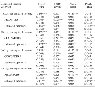
Using the specification with township fixed effects and controlling for outlook bias, we also examine the relative-income hypothesis separately for urban and rural residents. The results are presented in Table 4. First, we find that own income matters to health more for rural respondents, which makes sense since this population tends to be poorer. The estimated coefficients on estimated optimism are larger and more statistically significant for rural respondents for self-reported health, but the opposite is true for psychosocial health.
Turning to the coefficients on the subjective relative-income measures, we find the differences between urban and rural residents to be quite striking. For urban residents, the salience of classmates is the most important for both health outcomes, followed by relatives. Relative income with respect to classmates has a much larger impact on the health of urban residents (0.243 for SRHS and 0.166 for psychosocial health) than for the pooled sample (0.149 for SRHS and 0.093 for psychosocial health). The health impact of relative income with respect to relatives is also some-what larger for the urban sample (0.129 for SRHS and 0.121 for psychosocial health compared to 0.112 and 0.087 for the pooled sample). For urban residents, the impact of relative income with respect to coworkers and neighbors is much smaller in magnitude and statistically insignificant for both health outcomes. For SRHS, the lack of salience of neighbors contrasts with the results for the pooled sample, for which relative income with respect to neighbors is much larger (0.118 compared to -0.028 for the urban sample) and statistically significant.
geo-Table 4
OLS with Subjective Relative-Income Measures, by Subgroups
Dependent variable SRHS SRHS Psych. Psych.
Subgroup Rural Urban Rural Urban
(1) Log per-capita hh income 0.169*** 0.091 0.169*** 0.044 (0.045) (0.066) (0.033) (0.042)
RELATIVES 0.088* 0.129*** 0.058* 0.121***
(0.044) (0.045) (0.031) (0.029)
Estimated optimism 0.155** 0.046 0.056 0.063***
(0.060) (0.044) (0.036) (0.021) (2) Log per-capita hh income 0.191*** 0.067 0.181*** 0.035
(0.048) (0.058) (0.034) (0.051)
CLASSMATES 0.051 0.243*** 0.028 0.166**
(0.047) (0.064) (0.033) (0.068) Estimated optimism 0.173*** 0.010 0.071* 0.051*
(0.064) (0.039) (0.038) (0.030) (3) Log per-capita hh income 0.189*** 0.114 0.177*** 0.062
(0.048) (0.070) (0.032) (0.041)
COWORKERS 0.051 0.057 0.057 0.063
(0.058) (0.049) (0.045) (0.040) Estimated optimism 0.181*** 0.068 0.067* 0.083***
(0.065) (0.043) (0.035) (0.023) (4) Log per-capita hh income 0.127*** 0.135** 0.146*** 0.079**
(0.043) (0.058) (0.032) (0.033)
NEIGHBORS 0.208*** ⳮ0.028 0.119*** ⳮ0.008
(0.051) (0.083) (0.027) (0.079) Estimated optimism 0.117** 0.091** 0.034 0.102***
(0.057) (0.034) (0.035) (0.028)
(1) The sample size for rural areas is 1,377 when the dependent variable is SRHS and 1,379 when the dependent variable is psychosocial health. The sample size for urban areas is 1,514 when the dependent variable is SRHS and 1,516 when the dependent variable is psychosocial health.
(2) All regressions include as covariates the same set of nonincome variables reported in Table 2. All regressions control for township fixed effects.
(3) Standard errors are clustered by township.
(4) * significant at 10 percent; ** significant at 5 percent; *** significant at 1 percent.
graphic reference groups, in particular neighbors living in close proximity, are salient for rural residents, classmates, and relatives are more salient for urban residents.
their statistical significance and did not alter any of the main results on the impor-tance of different social reference groups.16
VI. Conclusion
In this paper, we examine for the first time the importance of social reference groups other than those defined on the basis of geographic or demographic characteristics. Our methodology advances the previous literature by controlling for unobserved regional omitted factors and demonstrating how subjective relative-in-come measurements can be used to test the importance of multiple social reference groups. We propose a method for controlling for unobserved reporting biases af-fecting both subjective relative-income measures and self-reported health.
Our results indicate that for urban residents, former classmates and relatives are important social reference groups in China. This demonstrates the importance of examining nongeographical reference groups in testing the relative deprivation hy-pothesis. In contrast to urban residents, geographic reference groups do appear to be salient for rural residents, especially neighbors who live in close proximity. These findings suggest that future research on the importance of more salient social ref-erence groups to health may hold great promise for improving understanding of how relative deprivation affects individual health outcomes, and that studies that overlook such comparison groups may be incomplete.
Future research on this topic can extend the current study in new directions. First, to avoid potential bias associated with self-reported health assessments, it will be more convincing to examine impacts on actual physical health measurements or more objective self-reported health outcomes, such as health expenditures, activities of daily life, or diagnosis of major diseases. Second, it will be of interest to study in greater depth the factors which explain variation in subjective relative-income measurements, both to account for possible reporting biases and to distinguish to what extent perceived relative-income differences are real or perceived, which is beyond the scope of the current study. Reporting biases can also be investigated through innovative survey questions, such as the use of vignettes. Finally, research on what determines how the salience of different social reference groups varies across individuals in the population can shed more light on the underlying social processes that determine individual health outcomes.
Appendix
Table A1
Psychosocial Health Index Questions (N⳱2,895)
Never Rarely Sometimes Often
No response
Worry about small things 826 763 908 374 25
28.5% 26.3% 31.4% 12.9% 0.9%
No appetite for food 1018 904 738 223 13
35.2% 31.2% 25.5% 7.7% 0.4%
Cannot focus attention 908 1021 727 171 68
31.4% 35.3% 25.1% 5.9% 2.4%
My life is a failure 1339 678 507 183 189
46.3% 23.4% 17.5% 6.3% 6.5%
Quality of sleep is poor 961 794 792 336 12
33.2% 27.4% 27.4% 11.6% 0.4%
I feel fortunate 216 447 1048 1119 65
7.5% 15.4% 36.2% 38.7% 2.2%
I feel alone 1172 863 590 171 100
40.5% 29.8% 20.4% 5.9% 3.4%
My life is very happy 169 368 1013 1282 63
58 127 35.0% 44.3% 2.2%
Table A2
Subjective Comparisons of Own Living Standards
Comparison
Relatives 45 380 1,502 707 226 2,860
1.57% 13.29% 52.52% 24.72% 7.90%
Classmates 37 265 1,255 511 173 2,241
1.65% 11.83% 56.00% 22.80% 7.72%
Coworkers 26 197 970 330 84 1,607
1.62% 12.26% 60.36% 20.54% 5.23%
Neighbors 50 437 1,568 576 140 2,771
1.80% 15.77% 56.59% 20.79% 5.05%
County 8 208 846 1,059 551 2,672
0.30% 7.78% 31.66% 39.63% 20.62%
Province 19 212 556 831 886 2,504
0.76% 8.47% 22.20% 33.19% 35.38%
Country 26 182 643 627 869 2,347
References
Benabou, Roland. 1996. “Equity and Efficiency in Human Capital Investment: the Local Connection.”Review of Economic Studies63(2): 237–64.
Conway, Terry, Ross Vickers, Harold Ward, and Richard Rahe. 1981. “Occupational Stress and Variation in Cigarette, Coffee, and Alcohol Consumption.”Journal of Health and Social Behavior22(2):155–65.
Daly, Mary C., Daniel J. Wilson, and Norman J. Johnson. 2007. “Relative Status and Well-Being: Evidence from U.S. Suicide Deaths.” Working Paper Series 2007–12, Federal Reserve Bank of San Francisco.
Davey Smith, George, Martin J. Shipley, and Geoffrey Rose. 1990. “The Magnitude and Causes of Socio-Economic Differentials in Mortality: Further Evidence from the Whitehall Study.”Journal of Epidemiology and Community Health44(4):265–70. Deaton, Angus, and Christina Paxson. 2001. “Mortality, Education, Income, and Inequality
among American Cohorts.” InThemes in the Economics of Aging, ed. David A. Wise, 129–70. Chicago: University of Chicago Press.
Deaton, Angus. 2003. “Health Inequality, and Economic Development.”Journal of Economic Literature41(1):113–58.
Deaton, Angus. 2002. “Policy Implications of the Gradient of Health and Wealth.”Health Affairs21(2):13–30.
Der, Geoff, Sally Macintyre, Graeme Ford, Kate Hunt, and Patrick West. 1999. “The Relationship of Household Income to a Range of Health Measures in Three Age Cohorts from the West Scotland.”European Journal of Public Health9(4):271–77
Easterlin, Richard. 1995. “Will Raising the Incomes of All Increase the Happiness of All?” Journal of Economic Behavior & Organization27(1): 35–47.
Eibner, Christine, and William N. Evans 2005. “Relative Deprivation, Poor Health Habits and Mortality.”Journal of Human Resources40(3):591–620.
Ferrer-i-Carbonell, Ada. 2005. “Income and Well-Being: An Empirical Analysis of the Comparison Income Effect.”Journal of Public Economics89(5–6):997–1019. Gerdtham, Ulf-G., and Magnus Johannesson. 2004. “Absolute Income, Relative Income,
Income Inequality, and Mortality.”Journal of Human Resources39(1):228–47. Gorman, Dennis. 1988. “Employment, Stressful Life Events and the Development of
Alcohol Dependence.”Drug and Alcohol Dependence22(1–2):151–59
Horwitz, Allan, and Lorraine Davies. 1994. “Are Emotional Distress and Alcohol Problems Differential Outcomes to Stress? An Exploratory Test.”Social Science Quarterly 75(3):607–21.
House, James, Karl Landis, and Debra Umberson. 1999. “Social Relationships and Health.” InThe Society and Population Health Reader: Income Inequality and Health, ed. Kawachi Ichiro, Bruce Kennedy, and Richard Wilkinson. 161–70. The New Press: New York.
Jensen, Robert, and Kaspar Richter. 2004. “The Health Implications of Social Security Failure: Evidence from the Russian Pension Crisis.”Journal of Public Economics88(1– 2): 209–36.
Kahneman, Daniel, Alan B. Krueger, David Schkade, Norbert Schwarz, and Arthur A. Stone 2006. “Would You Be Happier If You Were Richer? A Focusing Illusion.”Science 312(5782):1908–10.
Kennedy, Bruce, Ichiro Kawachi, Roberta Glass, and Deborah Prothrow-Stith. 1998. “Income Distribution, Socioeconomic Status, and Self Rated Health in the United States: Multilevel Analysis.”British Medical Journal317 (7163): 917–21.
Knight, Robert G., Sheila Williams, Rob McGee, and Susan Olaman. 1997. “Psychometric Properties of the Centre for Epidemiologic Studies Depression Scale (CES-D) in a Sample of Women in Middle Life.”Behaviour Research and Therapy35(4):373–80. Kristenson, Margareta, Kristina Orth-Gomer, Zita Kucinskiene, Bjorn Bergdahl, Henrikas
Calkauskas, Irena Balinkyniene, and Anders Olsson. 1999. “Attenuated Cortisol Response to a Standardized Stress Test in Lithuanian versus Swedish Men: the LiVicordia Study.” InThe Society and Population Health Reader: Income Inequality and Health, ed. Ichiro Kawachi, Bruce Kennedy, and Richard Wilkinson 433–43. The New Press: New York. Li, Zhonghe, and Madelyn Hsiao-Rei Hicks. 2010. “The CES-D in Chinese American
Women: Construct Validity, Diagnostic Validity for Major Depression, and Cultural Response Bias.”Psychiatry Research175(3):227–32.
Lin, Nan. 1989. “Measuring Depressive Symptomatology in China.”Journal of Nervous and Mental Disease177(3):121–31.
Lovallo, William. 1997.Stress and Health. Sage Publications: London.
Luttmer, Erzo F.P. 2005. “Neighbors as Negatives: Relative Earnings and Well-Being.” Quarterly Journal of Economics102(3):963–1002.
Lynch, John, and George Kaplan. 1999. “Understanding How Inequality in the Distribution of Income Affects Health.” InThe Society and Population Health Reader: Income Inequality and Health, ed. Ichiro Kawachi, Bruce Kennedy, and Richard Wilkinson. 202– 21. The New Press: New York.
Marmot, Michael, George Davey Smith, Stephen Stansfeld, Chadra Patel, Fiona North, J. Head, Ian White, Eric Brunner, and Amanda Feeny. 1991. “Health Inequalities among British Civil Servants: the Whitehall II Study.”Lancet337(8754):1387–93.
McBride, Michael. 2001. “Relative-Income Effects on Subjective Well-Being in the Cross-Section,”Journal of Economic Behavior & Organization45(3):251–78.
Mellor, Jennifer, and Jeffrey Milyo. 2002. “Income Inequality and Health Status in the United States: Evidence from the Current Population Survey.”Journal of Human Resources37(3):510–39.
Miller, Douglas, and Christina Paxson. 2006. “Relative Income, Race, and Mortality.” Journal of Health Economics25(5):979–1003.
Radloff, Lenore Sawyer. 1977. “The CES-D scale: A Self-Report Depression Scale for Research in the General Population.”Applied Psychological Measurement1(3):385–401. Shively, Carol, and Thomas Clarkson. 1999. “Social Status and Coronary Artery
Atherosclerosis in Female Monkeys.” InThe Society and Population Health Reader: Income Inequality and Health, ed. Ichiro Kawachi, Bruce Kennedy, and Richard Wilkinson. 393–404. The New Press: New York.
Shively, Carol, Kathy Laber-Laird, and Raymond Anton. 1999. “Behavior and Physiology of Social Stress and Depression in Female Cynomolgus Monkeys.” InThe Society and Population Health Reader: Income Inequality and Health, ed. Ichiro Kawachi, Bruce Kennedy, and Richard Wilkinson. 405–20. The New Press: New York.
Sapolsky, Robert. 1998.Why Zebras Don’t Get Ulcers. W. H. Freeman and Company: New York.
Sapolsky, Robert, Susan Alberts, and Jeanne Altmann. 1999. “Hypercortisolism Associated with Social Subordinance or Social Isolation among Wild Baboons.” InThe Society and Population Health Reader: Income Inequality and Health, ed. Ichiro Kawachi, Bruce Kennedy, and Richard Wilkinson. 421–32. The New Press: New York.
World Bank. 2009.From Poor Areas to Poor People: China’s Evolving Poverty Reduction Agenda. Washington, D.C.: The World Bank.