07350015%2E2014%2E907093

(1)

Full Terms & Conditions of access and use can be found at

http://www.tandfonline.com/action/journalInformation?journalCode=ubes20

Download by: [Universitas Maritim Raja Ali Haji], [UNIVERSITAS MARITIM RAJA ALI HAJI

TANJUNGPINANG, KEPULAUAN RIAU] Date: 11 January 2016, At: 20:22

Journal of Business & Economic Statistics

ISSN: 0735-0015 (Print) 1537-2707 (Online) Journal homepage: http://www.tandfonline.com/loi/ubes20

Identification and Efficient Estimation of

Simultaneous Equations Network Models

Xiaodong Liu

To cite this article: Xiaodong Liu (2014) Identification and Efficient Estimation of Simultaneous Equations Network Models, Journal of Business & Economic Statistics, 32:4, 516-536, DOI: 10.1080/07350015.2014.907093

To link to this article: http://dx.doi.org/10.1080/07350015.2014.907093

Accepted author version posted online: 24 Apr 2014.

Submit your article to this journal

Article views: 288

View related articles

(2)

Identification and Efficient Estimation of

Simultaneous Equations Network Models

Xiaodong L

IU

Department of Economics, University of Colorado, Boulder, CO 80309 (xiaodong.liu@colorado.edu)

This article considers identification and estimation of social network models in a system of simultaneous equations. We show that, with or without row-normalization of the social adjacency matrix, the network model has different equilibrium implications, needs different identification conditions, and requires differ-ent estimation strategies. When the adjacency matrix is not row-normalized, the variation in the Bonacich centrality across nodes in a network can be used as an IV to identify social interaction effects and improve estimation efficiency. The number of such IVs depends on the number of networks. When there are many networks in the data, the proposed estimators may have an asymptotic bias due to the presence of many IVs. We propose a bias-correction procedure for the many-instrument bias. Simulation experiments show that the bias-corrected estimators perform well in finite samples. We also provide an empirical example to illustrate the proposed estimation procedure.

KEY WORDS: Many-instrument bias; Social networks.

1. INTRODUCTION

Since the seminal work by Manski (1993), social network models have attracted a lot of attention (see Blume et al.2011, for a recent survey). In a social network model, agents inter-act with each other through network connections, which are captured by a social adjacency matrix. According to Manski (1993), an agent’s choice may be influenced by peers’ choices (the endogenous effect), by peers’ exogenous characteristics (the contextual effect), and/or by the common environment of the network (the correlated effect). It is the main interest of social network research to identify and estimate the different social interaction effects.

Manski (1993) considered a linear-in-means model, where the endogenous effect is based on the rational expectation of the choices of all agents in the network. Manski showed that the linear-in-means specification suffers from the “reflection prob-lem” so that endogenous and contextual effects cannot be sepa-rately identified. Lee (2007) introduced a model with multiple networks where an agent is equally influenced by all the other agents in the same network. Lee’s social network model can be identified by the variation in network sizes. The identification, however, can be weak if all of networks are large. Bramoull´e, Djebbari, and Fortin (2009) generalized Lee’s social network model to a generallocal-averagemodel, where endogenous and contextual effects are represented, respectively, by theaverage

choice andaveragecharacteristics of an agent’s connections (or friends).1 _{Based on the important observation that in a social}

network, an agent’s friend’s friend may not be a (direct) friend of that agent, Bramoull´e, Djebbari, and Fortin (2009) used the intransitivity in network connections as an exclusion restriction to identify different social interaction effects.

Liu and Lee (2010) considered the estimation of the local-aggregatesocial network model, where the endogenous effect is given by the aggregate choice of an agent’s friends. They showed that, for the local-aggregate model, different positions

1_{Bramoull´e, Djebbari, and Fortin (}₂₀₀₉_{) indicated that the first part of}

Proposi-tion 1 applies to arbitrary (non-row-normalized) adjacency matrices.

of the agents in a network captured by the Bonacich (1987) cen-trality can be used as an additional instrumental variable (IV) to improve estimation efficiency. Liu, Patacchini, and Zenou (2014) gave the identification condition for the local-aggregate model and showed that the condition is in general weaker than that for the local-average model derived by Bramoull´e, Djeb-bari, and Fortin (2009). They also proposed a J test for the specification of network models.

The aforementioned papers focus on single-equation network models involving only one activity. However, in real life, an agent’s decision usually involves more than one activity. For ample, a student may need to balance time between study and ex-tracurriculars and a firm may need to allocate resources between production and R&D (K¨onig, Liu, and Zenou2014). In a recent article, Cohen-Cole, Liu, and Zenou (2012) considered the iden-tification and estimation of local-average network models in the framework of simultaneous equations. Besides endogenous, contextual, and correlated effects as in single-equation network models, the simultaneous equations network model also incor-porates the simultaneity effect, where an agent’s choice in a certain activity may depend on his/her choice in a related activ-ity, andthe cross-activity peer effect, where an agent’s choice in a certain activity may depend on peers’ choices in a related activity. Cohen-Cole, Liu, and Zenou (2012) derived the identi-fication conditions for the various social interaction effects and generalize the spatial two-stage least-squares (2SLS) and three-stage least-squares (3SLS) estimators in Kelejian and Prucha (2004) to estimate the simultaneous equations network model.

In this article, we consider the identification and efficient estimation of the local-aggregate network model in a sys-tem of simultaneous equations. We show that, similar to the single-equation network model, the Bonacich centrality pro-vides additional information to achieve model identification and to improve estimation efficiency. We derive the identification

October 2014, Vol. 32, No. 4 DOI:10.1080/07350015.2014.907093

516

(3)

condition for the local-aggregate simultaneous equations net-work model, and show that the condition can be weaker than that for the local-average model. For efficient estimation, we suggest 2SLS and 3SLS estimators using additional IVs based on the Bonacich centrality of each network. As the number of such IVs depends on the number of networks, the 2SLS and 3SLS estimators would have an asymptotic many-instrument bias (Bekker1994) when there are many networks in the data. Hence, we propose a bias-correction procedure based on the es-timated leading-order term of the asymptotic bias. Monte Carlo experiments show that the bias-corrected estimators perform well in finite samples. We also provide an empirical example to illustrate the proposed estimation procedure.

The rest of the article is organized as follows. Section 2 introduces a network game which motivates the specification of the econometric model presented in Section3. Section4derives the identification conditions and Section5proposes 2SLS and 3SLS estimators for the model. The regularity assumptions and detailed proofs are given in the Appendix. Monte Carlo evidence on the finite sample performance of the proposed estimators is given in Section6. Section 7provides an empirical example. Section 8 briefly concludes.

2. THEORETICAL MODEL

2.1 The Network Game

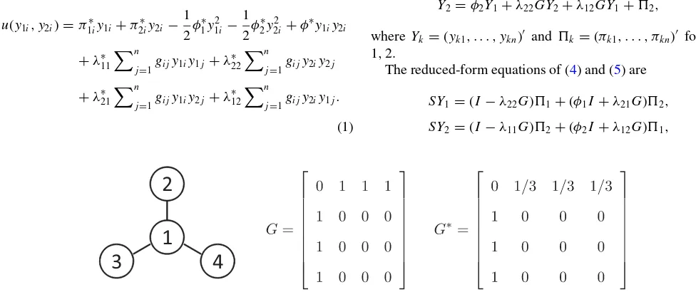
Suppose there is a finite set of agentsN _{= {}1, . . . , n_}in a network. We keep track of social connections in the network through its adjacency matrixG₌[gij]. If the network is

undi-rected, thenGis symmetric withgij =1 ifiandjare connected

andgij =0 otherwise. If the network is directed, thenGmay

be asymmetric withgij =1 if an arc is directed fromitojand gij =0 otherwise. Note that the undirected network can be

con-sidered as a special case of the directed network. LetG∗₌[g_ij∗] , withg_ij∗ ₌gij/

n

j=1gij, denote the row-normalized adjacency

matrix such that each row ofG∗_{adds up to 1.}_{Figure 1}_{gives an}

example ofGandG∗_{for an undirected star-shaped network.}

Given the network structure represented byG, agentichooses

y1i andy2i, the respective efforts of two related activities, to

maximize the following linear quadratic utility function:

u(y1i, y2i)=π1∗iy1i+π2∗iy2i−

1 2φ

∗ 1y

2 1i−

1 2φ

∗ 2y

2

2i+φ∗y1iy2i

+λ∗₁₁n

j=1gijy1iy1j +λ ∗ 22

n

j=1gijy2iy2j

+λ∗₂₁n

j=1gijy1iy2j +λ ∗ 12

n

j=1gijy2iy1j.

(1)

As in the standard linear-quadratic utility for a single activity model (Ballester, Calv´o-Armengol, and Zenou2006),π∗

1i and

π∗

2i capture ex ante individual heterogeneity. The cross-effects

between own efforts for different activities are given by

∂2u(y1i, y2i)

∂y1i∂y2i =

φ∗.

The cross-effects between own and peer efforts for the same activity are

∂2_u₍_y 1i, y2i)

∂y1i∂y1j =

λ∗₁₁gij and

∂2_u₍_y 1i, y2i)

∂y2i∂y2j =

λ∗₂₂gij,

which may indicate strategic substitutability or complementarity depending on the signs ofλ∗₁₁andλ∗₂₂. The cross-effects between own and peer efforts for different activities are given by

∂2_u₍_y 1i, y2i)

∂y1i∂y2j =

λ∗₂₁gij and

∂2_u₍_y 1i, y2i)

∂y2i∂y1j =

λ∗₁₂gij,

which may indicate strategic substitutability or complementarity depending on the signs ofλ∗₂₁andλ∗₁₂.

From the first-order conditions of utility maximization, we have thebest-response functions:

y1i =φ1y2i+λ11

n

j=1gijy1j +λ21

n

j=1gijy2j +π1i,

(2)

y2i =φ2y1i+λ22

n

j=1gijy2j +λ12

n

j=1gijy1j +π2i,

(3)

whereφ1=φ∗/φ1∗,φ2=φ∗/φ2∗,λ11=λ∗11/φ1∗,λ22=λ∗22/φ2∗,

λ21 =λ∗21/φ∗1, λ12=λ∗12/φ2∗, π1i=π1∗i/φ∗1, π2i =π2∗i/φ2∗. In (2) and (3), agent i’s best-response effort of a certain ac-tivity depends on the aggregate efforts of his/her friends of that activity and a related activity. Therefore, we call this model thelocal-aggregatenetwork game. In matrix form, the best-response functions are

Y1=φ1Y2+λ11GY1+λ21GY2+1, (4)

Y2=φ2Y1+λ22GY2+λ12GY1+2, (5)

where Yk=(yk1, . . . , ykn)′ and k=(πk1, . . . , πkn)′ for k=

1,2.

The reduced-form equations of (4) and (5) are

SY1=(I −λ22G)1+(φ1I +λ21G)2,

SY2=(I −λ11G)2+(φ2I +λ12G)1,

3

4

1

2

Figure 1. An example ofGandG∗_{for an undirected star-shaped network.}

(4)

whereIis a conformable identity matrix and

S ₌(1−φ1φ2)I−(λ11+λ22+φ1λ12+φ2λ21)G

+(λ11λ22−λ12λ21)G2. (6) If S is nonsingular (a sufficient condition for the nonsingu-larity of S is |ϕ1ϕ2| + |λ11+λ22+ϕ1λ12+ϕ2λ21| · ||G||∞+ |λ11λ22−λ12λ21| · ||G||2_∞<1, where || · ||∞ is the row-sum

matrix norm), then the local-aggregate network game has a unique Nash equilibrium in pure strategies with the equilibrium efforts given by

Y₁∗₌S−1[(I ₋λ22G)1+(φ1I +λ21G)2], (7)

Y₂∗₌S−1[(I ₋λ11G)2+(φ2I +λ12G)1]. (8)

2.2 Local Aggregate Versus Local Average: Equilibrium

Comparison

In a recent article, Cohen-Cole, Liu, and Zenou (2012) con-sidered a network game with utility function

u(y1i, y2i)=π1∗iy1i+π2∗iy2i−

1 2φ

∗ 1y

2 1i−

1 2φ

∗ 2y

2

2i+φ∗y1iy2i

+λ∗₁₁ n

j=1

g_ij∗y1iy1j +λ∗22

n

j=1

g_ij∗y2iy2j

+λ∗₂₁n j=1g

∗

ijy1iy2j+λ∗12

n

j=1g ∗

ijy2iy1j. (9)

From the first-order conditions of maximizing (9), the best-response functions of the network game are

y1i =φ1y2i+λ11

n

j₌1g ∗

ijy1j+λ21

n

j₌1g ∗

ijy2j +π1i,

y2i =φ2y1i+λ22

n

j=1g ∗

ijy2j+λ12

n

j=1g ∗

ijy1j +π2i,

or, in matrix form,

Y1=φ1Y2+λ11G∗Y1+λ21G∗Y2+1, (10)

Y2=φ2Y1+λ22G∗Y2+λ12G∗Y1+2. (11)

As G∗ is row-normalized, in (10) and (11), agent i’s best-response effort of a certain activity depends on the average

efforts of his/her friends of that activity and a related activity. Therefore, we call this model thelocal-averagenetwork game. Cohen-Cole, Liu, and Zenou (2012) showed that, ifS∗_is

non-singular, where

S∗ ₌(1−φ1φ2)I−(λ11+λ22+φ1λ12+φ2λ21)G∗

+(λ11λ22−λ12λ21)G∗2,

then the network game with payoffs (9) has a unique Nash equilibrium in pure strategies given by

Y₁∗₌S∗−1[(I₋λ22G∗)1+(φ1I+λ21G∗)2], (12)

Y₂∗₌S∗−1[(I₋λ11G∗)2+(φ2I+λ12G∗)1]. (13)

Although the best-response functions of the local-aggregate and local-average network games share similar functional forms, they have different implications. As pointed out by Liu, Patac-chini, and Zenou (2014), in the local-aggregate game, even if agents are ex ante identical in terms of individual attributes

1and2, agents with different positions in the network would have different equilibrium payoffs. On the other hand, the local-averagegame is based on the mechanism of social conformism. Liu, Patacchini, and Zenou (2014) showed that the best-response function of the local-average network game can be derived from a setting where an agent will be punished if he deviates from the “social norm” (the average behavior of his friends). Therefore, if the agents are identical ex ante, they would behave the same in equilibrium.

To illustrate this point, suppose the agents in a network are ex ante identical such that 1=π1ln and2=π2ln, where π1, π2are constant scalars andlnis ann×1 vector of ones. As G∗_l

n=G∗2ln=ln, it follows from (12) and (13) thatY1∗=c1ln

andY∗

2 =c2ln, where

c1 =[(1−λ22)π1+(φ1+λ21)π2]/[(1−φ1φ2)

−(λ11+λ22+φ1λ12+φ2λ21)+(λ11λ22−λ12λ21)],

c2 =[(1−λ11)π2+(φ2+λ12)π1]/[(1−φ1φ2)

−(λ11+λ22+φ1λ12+φ2λ21)+(λ11λ22−λ12λ21)]. Thus, for the local-average network game, the equilibrium ef-forts and payoffs are the same for all agents. On the other hand, for the local-aggregate network game, it follows from (7) and (8) that

Y₁∗ ₌S−1[(I₋λ22G)π1+(φ1I+λ21G)π2]ln, Y₂∗ ₌S−1[(I₋λ11G)π2+(φ2I+λ12G)π1]ln.

Thus, the agents would have different equilibrium efforts and payoffs if Gln is not proportional to ln, that is agents have

different number of friends.

Therefore, the local-aggregate and local-average network games have different equilibrium and policy implications. Un-derstanding the different microfoundations of the two models, including their different equilibrium implications, may help us to understand which model is more appropriate for a cer-tain economic context.2 The following sections show that the econometric model for the local-aggregate network game has some interesting features that requires different identification conditions and estimation methods from those for the local-average model studied by Cohen-Cole, Liu, and Zenou (2012).

3. ECONOMETRIC MODEL

3.1 The Local-Aggregate Simultaneous Equations

Network Model

The econometric network model follows the best-response functions (4) and (5). Suppose thenobservations in the data are partitioned into ¯rnetworks, withnr agents in therth network.

For therth network, let

1,r=Xrβ1+GrXrγ1+α1,rlnr +ǫ1,r,

2,r=Xrβ2+GrXrγ2+α2,rlnr +ǫ2,r.

2_{It may not always be obvious to see whether the local-average or local-aggregate}

model is more appropriate just by economic intuition. Sometimes, a specification test is needed. Liu, Patacchini, and Zenou (2014) extended theJtest to network models.

(5)

whereXris annr×kxmatrix of exogenous variables,Gris the

adjacency matrix of networkr,lnr is annr×1 vector of ones, andǫ1,r, ǫ2,rarenr×1 vectors of disturbances. The

specifica-tion of1,rand2,ris quite common for network models (see,

e.g., Bramoull´e, Djebbari, and Fortin2009; Calv´o-Armengol, Patacchini, and Zenou 2009; Liu and Lee 2010). In spatial econometrics literature, this specification is known as the spatial Durbin model (LeSage and Pace2009). Essentially, this model specification imposes exclusion restrictions such that1,r and 2,r do not depend on the characteristics of indirect

connec-tions. It follows by (4) and (5) that Y1,r andY2,r, which are nr×1 vectors of observed choices of two related activities for

the agents in therth network, are given by

Y1,r =φ1Y2,r+λ11GrY1,r+λ21GrY2,r+Xrβ1+GrXrγ1

+α1,rlnr+ǫ1,r,

Y2,r =φ2Y1,r+λ22GrY2,r+λ12GrY1,r+Xrβ2+GrXrγ2

+α2,rlnr+ǫ2,r.

Let diag{As} denote a “generalized” block diagonal

ma-trix with diagonal blocks being ns×ms matrices As’s. For k₌1,2, let Yk =(Yk,′1, . . . , Yk,′r¯)′, X=(X1′, . . . , Xr′¯)′, αk=

(αk,1, . . . , αk,r¯)′, ǫk=(ǫk,′1, . . . , ǫ′k,r¯)′, L=diag{lnr}

¯

r r=1 and

G₌diag{Gr}rr¯=1. Then, for all the ¯rnetworks,

Y1 =φ1Y2+λ11GY1+λ21GY2+Xβ1+GXγ1+Lα1+ǫ1,

(14)

Y2 =φ2Y1+λ22GY2+λ12GY1+Xβ2+GXγ2+Lα2+ǫ2.

(15) For ǫ1=(ǫ11, . . . , ǫ1n)′ and ǫ2=(ǫ21, . . . , ǫ2n)′, we assume

E(ǫ1i)=E(ǫ2i)=0, E(ǫ12i)=σ12, and E(ǫ22i)=σ22. Further-more, we allow the disturbances of the same agent to be correlated across equations by assuming E(ǫ1iǫ2i)=σ12 and E(ǫ1iǫ2j)=0 fori=j. WhenSgiven by (6) is nonsingular, the

reduced-form equations of the model are

Y1 =S−1[X(φ1β2+β1)+GX(λ21β2−λ22β1+φ1γ2+γ1) +G2X(λ21γ2−λ22γ1)+L(φ1α2+α1)

+GL(λ21α2−λ22α1)]+S−1u1, (16)

Y2 =S−1[X(φ2β1+β2)+GX(λ12β1−λ11β2+φ2γ1+γ2) +G2X(λ12γ1−λ11γ2)+L(φ2α1+α2)

+GL(λ12α1−λ11α2)]+S−1u2, (17) where

u1=(I−λ22G)ǫ1+(φ1I +λ21G)ǫ2, (18)

u2=(I−λ11G)ǫ2+(φ2I +λ12G)ǫ1. (19)

In this model, we allow network-specific effectsα1,randα2,r

to depend on X and G by treating α1 and α2 as ¯r×1 vec-tors of unknown parameters (as in a fixed-effect panel data model). When the number of network ¯r is large, we may have the “incidental parameter” problem (Neyman and Scott1948). To avoid this problem, we transform (14) and (15) using a deviation from group mean projector J ₌diag{Jr}rr¯=1 where

Jr =Inr−

1

nrlnrl

′

nr . This transformation is analogous to the “within” transformation for fixed-effect panel data models. As

JL₌0, the transformed equations are

JY1 =φ1JY2+λ11JGY1+λ21JGY2+JXβ1

+JGXγ1+J ǫ1, (20)

JY2 =φ2JY1+λ22JGY2+λ12JGY1+JXβ2

+JGXγ2+J ǫ2. (21)

Our identification results and estimation methods are based on the transformed model.

3.2 Identification Challenges

Analogous to the local-average simultaneous equations net-work model studied by Cohen-Cole, Liu, and Zenou (2012), the local-aggregate simultaneous equations network model given by (14) and (15) incorporates (within-activity) endogenous ef-fects, contextual efef-fects, simultaneity efef-fects, cross-activity peer effects, network-correlated effects, and cross-activity correlated effects. It is the main purpose of this article to establish identifi-cation conditions and propose efficient estimation methods for the various social interaction effects.

3.2.1 Endogenous Effect and Contextual Effect. The en-dogenous effect, where an agent’s choice may depend on choices of his/her friends in the same activity, is captured by the coef-ficients λ11 andλ22. The contextual effect, where an agent’s choice may depend on the exogenous characteristics of his/her friends, is captured byγ1andγ2.

The nonidentification of a social interaction model caused by the coexistence of those two effects is known as the “reflection problem” (Manski 1993). For example, in a linear-in-means model, where an agent is equally affected by all the other agents in the network and by nobody outside the network, the mean of endogenous regressor is perfectly collinear with the exogenous regressors. Hence, endogenous and contextual effects cannot be separately identified.

In reality, an agent may not be evenly influenced by all the other agents in a network. In a network model, it is usually as-sumed that an agent is directly influenced only by his/her friends. Note that, if individualsi, j are friends andj, kare friends, it does not necessarily imply thati, k are also friends. Thus, the intransitivity in network connections provides an exclusion re-striction to identify the model. Bramoull´e, Djebbari, and Fortin (2009) showed that if intransitivities exist in a network so that

I, G∗_{, G}∗2

are linearly independent, then the characteristics of an agent’s second-order (indirect) friendsG∗2Xcan be used as IVs to identify the endogenous effect from the contextual effect in thelocal-averagemodel.3

On the other hand, when Gr does not have constant row

sums, the number of friends represented by the element ofGrlnr varies across agents. For alocal-aggregatemodel, Liu and Lee (2010) showed that the Bonacich (1987) centrality, which has

Grlnr as the leading-order term, can also be used as an IV

3_{A stronger identification condition is needed if the network fixed effect is also}

included in the model.

(6)

for the endogenous effect. For the alocal-aggregateseemingly unrelated regression (SUR) network model with fixed network effect, we show in the following section that identification is possible through the intransitivity in network connections and/or the variation in Bonacich centrality.

3.2.2 Simultaneity Effect and Cross-Activity Peer Effect. The simultaneity effect, where an agent’s choice in an activ-ity may depend on his/her choice in a related activactiv-ity, can be seen in the coefficientsφ1andφ2. The cross-activity peer effect, where an agent’s choice may depend on those of his/her friends in a related activity, is represented by the coefficientsλ21 and

λ12.

For a standard simultaneous equations model without social interaction effects, simultaneity leads to a well-known iden-tification problem and the usual remedy is to impose exclu-sion restrictions on the exogenous variables. Cohen-Cole, Liu, and Zenou (2012) showed that, with the simultaneity effector

the cross-activity peer effect (but not both), thelocal-average

network model can be identified without imposing any exclu-sion restrictions onX, as long asJ, J G∗_{, J G}∗2_{, J G}_∗3

are lin-early independent. In this article, we show that, by exploiting the variation in Bonacich centrality, the local-aggregate net-work model with the simultaneity effect or the cross-activity peer effect (but not both) can be identified under weaker conditions.

However, neither the intransitivity inGnor the variation in Bonacich centrality would be enough to identify the simultane-ous equations network model with both simultaneity and cross-activity peer effects. One possible approach to achieve identifi-cation is to impose exclusion restrictions onX. We show that, with exclusion restrictions onX, the local-aggregatenetwork model with both simultaneity and cross-activity peer effects can be identified under weaker conditions than the local-average

model.

3.2.3 Network Correlated Effect and Cross-Activity Corre-lated Effect. Furthermore, the structure of the simultaneous equations network model is flexible enough to allow us to in-corporate two types of correlated effects.

First, the network fixed effect given by α1,r andα2,r

cap-tures the network correlated effect where agents in the same network may behave similarly as they have similar unobserved individual characteristics or they face similar institutional envi-ronment. Therefore, the network fixed-effect serves as a (partial) remedy for the selection bias that originates from the possible sorting of agents with similar unobserved characteristics into a network.

Second, in the simultaneous equations network model, the error terms of the same agent is allowed to be correlated across equations. The correlation structure of the error term captures

the cross-activity correlated effect so that the choices of the same agent in related activities could be correlated. As our iden-tification results are based on the mean of reduce-form equa-tions, they are not affected by the correlation structure of the error term. However, for estimation efficiency, it is important to take into account the correlation in the disturbances. The estimators proposed in this article extend the generalized spa-tial 3SLS estimator in Kelejian and Prucha (2004) to estimate the simultaneous equations network model in the presence of many IVs.

4. IDENTIFICATION RESULTS

Among the regularity assumptions listed in AppendixA, As-sumption 4 is a sufficient condition for identification of the simultaneous equations network model. LetZ1andZ2denote the matrices of right-hand side (RHS) variables of (14) and (15). For Assumption 4 to hold, E(J Z1) and E(J Z2) need to have full column rank for large enough n. In this section, we provide sufficient conditions for E(J Z1) to have full column rank. The sufficient conditions for E(J Z2) to have full column rank can be analogously derived.

In this article, we focus on the case whereGr does not have

constant row sums for some networkr. WhenGr has constant

column sums for allr, the equilibrium implication of the local-aggregate network game is similar to that of the local-average network game and the identification conditions are analogous to those given in Cohen-Cole, Liu, and Zenou (2012). Henceforth, letρandη(possibly with subscripts) denote some generic con-stant scalars that may take different values for different uses. For ease of presentation, we assumeGandXare nonstochastic. Furthermore, in this section, we assumeXis a column vector.

4.1 Identification of the SUR Network Model

First, we consider the seemingly unrelated regression (SUR) network model whereφ1=φ2=λ21=λ12 =0. Thus, (4) and (5) become

Y1=λ11GY1+Xβ1+GXγ1+Lα1+ǫ1, (22)

Y2=λ22GY2+Xβ2+GXγ2+Lα2+ǫ2. (23)

For the SUR network model, an agent’s choice is still allowed to be correlated with his/her own choices in related activities through the correlation structure of the disturbances. Whenφ1 =

φ2=λ21 =λ12=0, it follows from the reduced-form equation (16) that

E(Y1)=(I−λ11G)−1(Xβ1+GXγ1+Lα1). (24)

For (22), let Z1=[GY1, X, GX]. Identification of (22) re-quires E(J Z1)=[E(J GY1), J X, J GX] to have full column rank. As (I₋λ11G)−1=I+λ11G(I−λ11G)−1 and (I −

λ11G)−1G=G(I −λ11G)−1, it follows from (24) that

E(J GY1)=J GXβ1+J G2(I −λ11G)−1X(λ11β1

+γ1)+J G(I−λ11G)−1Lα1.

Ifλ11β1+γ1=0,J G2(I −λ11G)−1X, with the leading order termJ G2X, can be used as IVs for the endogenous regressor

J GY1. On the other hand, ifGrdoes not have constant row sums

for allr₌1, . . . ,r¯, thenJ G(I₋λ11G)−1L=0. As pointed out by Liu and Lee (2010), the Bonacich centrality given by

G(I₋λ11G)−1L, with the leading order termGL, can be used as additional IVs for identification. The following proposition

(7)

1

2

3

Figure 2. An example where the local-aggregate model can be iden-tified by Proposition 1(ii).

gives a sufficient condition for E(J Z1) to have full column rank.

Proposition 1. Suppose Gr has nonconstant row sums for

some network r. For Equation (22), E(J Z1) has full column rank if

(i)α1,r=0 orλ11β1+γ1=0, andInr, Gr, G

2

r are linearly

independent; or (ii)G2

r =ρ1Inr+ρ2Gr andα1,r(1−ρ2λ11−ρ1λ

2 11)=0. The identification condition for the local-aggregate SUR model given in Proposition 1 is, in general, weaker than that for thelocal-average SUR model. As pointed out by Bramoull´e, Djebbari, and Fortin (2009),4_{identification of the local-average}

model requires the linear independence ofI, G∗_{, G}∗2_{, G}∗3_. Con-sider a dataset with ¯r networks, where all networks in the data are represented by the graph inFigure 1. For the ¯r networks,

G₌diag{Gr}rr¯=1 whereGr is given by the adjacency matrix

inFigure 1. For the row-normalized adjacency matrixG∗, it is easy to see that G∗3 ₌G∗. Therefore, it follows by Proposi-tion 5 of Bramoull´e, Djebbari, and Fortin (2009) that the local-average SUR model is not identified. On the other hand, for the network in Figure 1, Gr has nonconstant row sums and I4, Gr, G2rare linearly independent. Hence, by Proposition 1(i),

the local-aggregate SUR model can be identified ifα1,r =0 or

λ11β1+γ1=0.

Figure 2gives an example where the condition in Proposition 1(ii) is satisfied. For the directed graph inFigure 2, it is easy to see thatG2

r =ρ1I3+ρ2Gr forρ1=ρ2=0. As the row sums ofGrare not constant, by Proposition 1(ii), the local-aggregate

SUR model is identified ifα1,r=0.

The following corollary shows that for a network with sym-metric adjacency matrixGr, the local-aggregate SUR model can

be identified ifGrhas nonconstant row sums.

Corollary 1. Supposeλ11β1+γ1=0 orα1,r=0 for some

networkr. Then, for Equation (22), E(J Z1) has full column rank ifGris symmetric and has nonconstant row sums.

4.2 Identification of the Simultaneous Equations

Network Model

4.2.1 Identification Under the Restrictionsλ21=λ12=0. For the simultaneous equations network model, besides the en-dogenous, contextual, and correlated effects, first we incorporate

4_{As the identification conditions given in Bramoull´e, Djebbari, and Fortin (}₂₀₀₉₎

are based on the mean of reduce-form equations, they are not affected by the correlation structure of the error term. Hence, they can be applied to the SUR model.

the simultaneity effect so that an agent’s choice is allowed to de-pend on his/her own choice in a related activity. However, we as-sume that an agent’s choice is not affected by the friends’ choices in related activities. Under the restrictionsλ21=λ12 =0, (14) and (15) become

Y1=φ1Y2+λ11GY1+Xβ1+GXγ1+Lα1+ǫ1, (25)

Y2=φ2Y1+λ22GY2+Xβ2+GXγ2+Lα2+ǫ2. (26)

For (25), letZ1 =[Y2, GY1, X, GX]. For identification of the simultaneous equations model, E(J Z1) is required to have full column rank for large enoughn. The following proposition gives sufficient conditions for E(J Z1) to have full column rank.

Proposition 2. SupposeGr has nonconstant row sums and Inr, Gr, G

2

r are linearly independent for some networkr.

• When [lnr, Grlnr, G

2

rlnr] has full column rank, E(J Z1) of Equation (25) has full column rank if

(i) Inr, Gr, G

2

r, G3rare linearly independent andD1given by (B.1) has full rank; or

(ii) G3

r =ρ1Inr+ρ2Gr+ρ3G

2

r andD1∗ given by (B.2) has full rank.

• WhenG2_rlnr =η1lnr +η2Grlnr, E(J Z1) of Equation (25) has full column rank if

(iii) Inr, Gr, G

2

r, G3r are linearly independent and D

†

1 given by (B.3) has full rank; or

(iv) G3_r ₌ρ1Inr+ρ2Gr+ρ3G

2

r andD

‡

1 given by (B.4) has full rank.

Cohen-Cole, Liu, and Zenou (2012) showed that a suf-ficient condition to identify the local-average simultaneous equations model under the restrictionsλ21=λ12 =0 requires

that J, J G∗_{, J G}∗2_{, J G}∗3 _{are linearly independent. The}

suf-ficient conditions to identify the restricted local-aggregate

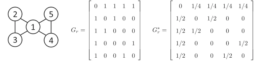
simultaneous equations model given by Proposition 2 are weaker in general. Consider a dataset, where all networks are given by the graph in Figure 3. It is easy to see that, for the row-normalized adjacency matrix G∗₌_diag_{_G∗

r}

¯

r r=1, where G∗

r is given in Figure 3, G∗

3

= −14I+ 1

4G∗+G∗ 2

. Therefore, the condition to identify the local-average model does not hold. On the other hand, for the rth network in the data, G2_rl5=4l5+Gl5. As the row sums of Gr are

not constant and I5, Gr, G2r, G

3

r are linearly independent,

the local-aggregate model can be identified according to Proposition 2(iii).

For another example where identification is possible for the local-aggregate model but not for the local-average model, let us revisit the network given by the graph inFigure 1. For a dataset with ¯rsuch networks, asG∗3

=G∗_{, the condition to identify the}

local-average simultaneous equations model given by Cohen-Cole, Liu, and Zenou (2012) does not hold. On the other hand, for the adjacency matrix without row-normalization,G3

r =3Gr

andG2_rl4=3l4. As the row sums ofGr are not constant and I4, Gr, G2r are linearly independent, the local-aggregate

simul-taneous equations model can be identified according to Propo-sition 2(iv).

(8)

3

5

2

4

1

Figure 3. An example where the local-aggregate model can be identified by Proposition 2(iii).

Figure 4provides an example where the condition in Propo-sition 2(ii) is satisfied. For the directed network in Figure 4,

G3_r ₌0. As [l3, Grl3, G2rl3] has full column rank andI3, Gr, G2r

are linearly independent, the local-aggregate simultaneous equa-tions model can be identified according to Proposition 2(ii).

4.2.2 Identification Under the Restrictions φ1=φ2=0. Next, let us consider the simultaneous equations model where an agent’s choice is allowed to depend on his/her friends’ choices of the same activity and a related activity. This specification incorporates the endogenous, contextual, correlated, and cross-activity peer effects, but excludes the simultaneity effect. Under the restrictionsφ1=φ2=0, (14) and (15) become

Y1=λ11GY1+λ21GY2+Xβ1+GXγ1+Lα1+ǫ1, (27)

Y2=λ22GY2+λ12GY1+Xβ2+GXγ2+Lα2+ǫ2. (28)

For (27), letZ1 =[GY1, GY2, X, GX]. The following proposi-tion gives sufficient condiproposi-tions for E(J Z1) to have full column rank.

Proposition 3. SupposeGr has nonconstant row sums and Inr, Gr, G

2

rare linearly independent for some networkr.

2

(i) Inr, Gr, G

2

r, G

3

rare linearly independent andD2given by (B.5) has full rank; or

(ii) G3_r ₌ρ1Inr+ρ2Gr+ρ3G

2

r andD2∗ given by (B.6) has full rank.

• WhenG2_rlnr =η1lnr+η2Grlnr, E(J Z1) of Equation (27) has full column rank if

(iii) Inr, Gr, G

2

r, G3r are linearly independent and D

†

2 given by (B.7) has full rank; or

(iv) G3

r =ρ1Inr+ρ2Gr+ρ3G

2

r andD

‡

2 given by (B.8) has full rank.

1

2

3

Figure 4. An example where the local-aggregate model can be iden-tified by Proposition 2(ii).

For the local-average simultaneous equations model un-der the restrictionsφ1=φ2=0, Cohen-Cole, Liu, and Zenou (2012) gave a sufficient identification condition that requires

J, J G∗, J G∗2, J G∗3to be linearly independent. The sufficient

identification conditions for thelocal-aggregatemodel given by Proposition 3 are weaker in general. As explained in the preced-ing section, for the network given by the graph in Figures1or 3, the identification condition for the local-average model does not hold. On the other hand, ifGris given byFigure 3, the

local-aggregate model can be identified according to Proposition 3(iii) since the row sums ofGr are not constant,G2rl5=4l5+Gl5, andI5, Gr, G2r, G3r are linearly independent. Similarly, ifGris

given byFigure 1, the local-aggregate model can be identified according to Proposition 3 (iv) since the row sums ofGrare not

constant,G2

rl4=3l4 ,G3r =3Gr, and I4, Gr, G2r are linearly

independent.

4.2.3 Nonidentification of the General Simultaneous Equa-tions Model. For the general simultaneous equations model given by (14) and (15), the various social interaction effects can-not be separately identified through the mean of the RHS vari-ables without imposing any exclusion restrictions. This is be-cause E( ¯Z1) and E( ¯Z2), where ¯Z1=[Y2, GY1, GY2, X, GX, L] and ¯Z2 =[Y2, GY1, GY2, X, GX, L], do not have full column rank as shown in the following proposition.

Proposition 4. For (14) and (15), E( ¯Z1) and E( ¯Z2) do not have full column rank.

Proposition 4 shows that, for the general simultaneous equa-tions model with both simultaneity and cross-activity peer ef-fects, exploiting the intransitivities in social connections and/or variations in Bonacich centrality does not provide enough exclusion restrictions for identification. One way to achieve identification is to impose exclusion restrictions on the exoge-nous variables. Consider the following model

Y1=φ1Y2+λ11GY1+λ21GY2+X1β1+GX1γ1

+Lα1+ǫ1, (29)

Y2=φ2Y1+λ22GY2+λ12GY1+X2β2+GX2γ2

+Lα2+ǫ2, (30)

where, for ease of presentation, we assume X1, X2 are vec-tors and [X1, X2] has full column rank. From the reduced-form

(9)

Equations (16) and (17), we have sufficient conditions for E(J Z1) to have full column rank.

Proposition 5. Suppose Gr has nonconstant row sums for

some networkr.

2

(i) Inr, Gr, G

2

r, G

3

rare linearly independent andD3given by (B.9) has full rank; or

r are linearly independent and D

†

3 given by (B.11) has full rank;

(iv) Inr, Gr, G

2

r are linearly independent,G3r =ρ1Inr +

ρ2Gr+ρ3G2r andD

‡

3given by (B.12) has full rank; or

(v) G2_r ₌η1Inr+η2Gr andD

♯

3given by (B.13) has full rank.

For the generallocal-averagesimultaneous equations model, Cohen-Cole, Liu, and Zenou (2012) provided a sufficient iden-tification condition that requires J, J G∗, J G∗2 to be linearly independent. SupposeG∗ ₌_diag_{_G∗

identification condition for the local-average model does not hold. On the other hand, as Gr given by Figure 1 has

non-constant row sums andI4, Gr, G2r are linearly independent, the

local-aggregate model given by (29) and (30) can be identified according to Proposition 5(iv).

5. ESTIMATION

5.1 The 2SLS Estimator With Many IVs

The general simultaneous equations model given by (29) and (30) can be written more compactly as

Y1=Z1δ1+Lα1+ǫ1 and Y2=Z2δ2+Lα2+ǫ2, (33) respectively (Lee2003). However, bothF1andF2are infeasible as they involve unknown parameters. Hence, we use linear com-binations of feasible IVs to approximateF1andF2as in Kelejian and Prucha (2004) and Liu and Lee (2010). Let ¯G₌φ1φ2I+ approximation error of pj=0G¯j diminishes in a geometric rate as p_{→ ∞}. Sincep_j₌₀G¯j _{can be considered as a}

lin-ear combination of [I, G, . . . , G2p], the best IVs F1 andF2 can be approximated by a linear combination of ann_×K IV matrix

QK =J[X1, GX1, . . . , G2p+3X1, X2, GX2, . . . , G2p+3X2,

GL, . . . , G2p+2L] (35)

with an approximation error diminishing very fast whenK(or

p) goes to infinity, as required by Assumption 5 in Appendix A. Let PK =QK(QK′ QK)−Q′K. The many-instrument 2SLS

estimators forδ1 andδ2are ˆδ1,2sls=(Z1′PKZ1)−1Z1′PKY1and ˆ

δ2,2sls =(Z′2PKZ2)−1Z′2PKY2.5

Let H11=limn→∞1nF1′F1 and H22 =limn→∞1nF2′F2. The following proposition establishes the consistency and asymp-totic normality of the many-instrument 2SLS estimator.

Proposition 6. Under Assumptions 1–5, if K_{→ ∞} and

K/n_→0, then√n( ˆδ1,2sls−δ1−b1,2sls)

From Proposition 6, when the number of IVs K grows at a rate slower than the sample sizen, the 2SLS estimators are consistent and asymptotically normal. However, the asymptotic distribution of the 2SLS estimator may not center around the true parameter value due to the presence of many-instrument bias (see, e.g., Bekker1994). IfK2/n_→0, then√nb1,2sls

→0 and the 2SLS estimators are properly centered.

5_{The finite sample properties of IV-based estimators can be sensitive to the}

number of IVs. In a recent article, Liu and Lee (2013) derived the Nagar-type approximate MSE of the 2SLS estimator for spatial models, which can be minimized to choose the optimal number of IVs as in Donald and Newey (2001) . The approximate MSE can be derived in a similar way for the proposed estimators in the article.

(10)

The condition that K/n_→0 is crucial for the 2SLS es-timator to be consistent. To see this, we look at the first-order conditions of the 2SLS, 1_nZ′

1PK(Y1−Z1δˆ1,2sls)=0 and, thus, the 2SLS estimators may not be consistent, if the number of IVs grows at the same or a faster rate than the sample size.

Note that the submatrixGLin the IV matrixQK given by

(35) has ¯rcolumns, where ¯ris the number of networks. Hence,

K/n_→0 implies ¯r/n₌1/n¯r →0, where ¯nr =n/r¯is the

av-erage network size. So, for the 2SLS estimator with the IV matrix

QKto be consistent, the average network size needs to be large.

On the other hand,K2/n_→0 implies ¯r2/n₌r/¯ n¯r →0. So,

for the 2SLS estimator to be properly centered, the average net-work size needs to be large relative to the number of netnet-works. The many-instrument bias of the 2SLS estimator can be corrected by the estimated leading-order biases b1,2sls and

b2,2sls given in Proposition 6. Let ˜δ1=( ˜φ1,λ˜11,λ˜21,β˜1′,γ˜1′)′ and ˜δ2 =( ˜φ2,λ˜22,λ˜12,β˜2′,γ˜2′)′ be

√

n-consistent preliminary 2SLS estimators based on a fixed number of IVs (e.g.,

Q₌J[X1, GX1, G2X1, X2, GX2, G2X2]). Let ˜ǫ1=J(Y1−

Z1δ˜1) and ˜ǫ2=J(Y2−Z2δ˜2). The leading-order biases can be estimated by ˆb1,2sls=(Z′1PKZ1)−1E(ˆ U1′PKǫ1) and ˆb2,2sls= (Z′

2PKZ2)−1E(ˆ U2′PKǫ2), where ˆE(U1′PKǫ1) and ˆE(U2′PKǫ2) are obtained by replacing the unknown parameters in (36) and (37) by ˜δ1,δ˜2and

˜

σ₁2₌ǫ˜₁′ǫ˜1/(n−r¯), σ˜12=ǫ˜′2ǫ˜2/(n−r¯), σˆ12 =ǫ˜1′ǫ˜2/(n−r¯). (38)

The bias-corrected 2SLS (BC2SLS) estimators are given by ˆ

δ1,bc2sls=δˆ1,2sls−bˆ1,2slsand ˆδ2,bc2sls=δˆ2,2sls−bˆ2,2sls.

Proposition 7. Under Assumptions 1–5, if K_{→ ∞}

and K/n_→0, then √n( ˆδ1,bc2sls−δ1)

lows that the BC2SLS estimators have properly centered asymp-totic normal distributions as long as the average network size ¯nr

is large.

5.2 The 3SLS Estimator With Many IVs

The 2SLS and BC2SLS estimators consider equation-by-equation estimation and are inefficient as they do not make use of the cross-equation correlation in the disturbances. To fully use the information in the system, we extend the 3SLS estimator proposed by Kelejian and Prucha (2004) to estimate the local-aggregate network model in the presence of many IVs.

We stack the equations in the system (33) as

Y ₌Zδ₊(I2⊗L)α+ǫ,

⊗I)F. The following proposition gives the asymptotic distribution of the many-instrument 3SLS estimator.

K/n_→0, then

Similar to the 2SLS estimator, when the number of IVs goes to infinity at a rate slower than the sample size, the 3SLS estimator

(11)

is consistent and asymptotically normal with an asymptotic bias given by√nb3sls. IfK2/n→0, then√nb3sls

p

→0 and the 3SLS estimator is properly centered and efficient as the covariance matrixH−1 _{attains the efficiency lower bound for the class of} IV estimators.

The leading-order asymptotic bias of the 3SLS estimator given in Proposition 8 can be estimated to correct the many-instrument bias. Let the estimated bias be

ˆ

b3sls=[Z′( ˜−1⊗PK)Z]−1E[U′(−1⊗PK)ǫ],

where ˜ is given by (39) andE[U′(−1_⊗PK)ǫ] is obtained

by replacing the unknown parameters in (40) by√n-consistent preliminary 2SLS estimators ˜δ1and ˜δ2. The bias-corrected 3SLS (BC3SLS) estimator is given by ˆδbc3sls =δˆ3sls−bˆ3sls. The fol-lowing proposition shows that the BC3SLS estimator is properly centered and asymptotically efficient if the number of IVs in-creases slower than the sample size.

K/n_→0, then √

n( ˆδbc3sls−δ)

d

→N(0, H−1).

6. MONTE CARLO EXPERIMENTS

To investigate the finite sample performance of the 2SLS and 3SLS estimators, we conduct a limited simulation study based on the following model

Y1 =φ1Y2+λ11GY1+λ21GY2+X1β1+GX1γ1+Lα1+ǫ1,

(41)

Y2 =φ2Y1+λ22GY2+λ12GY1+X2β2+GX2γ2+Lα2+ǫ2.

(42)

For the experiment, we consider four samples with different numbers of networks ¯rand network sizesnr. Samples 1, 2, and

3 have ¯r₌30 equal-sized networks withnr =10,nr =15 and nr =30 respectively. Sample 4 has ¯r=60 equal-sized networks

withnr =15 . For each network, the adjacency matrixGr is

generated in a similar way as in Liu and Lee (2010). First, for theith row of Gr (i=1, . . . , nr), we generate an integer pri

uniformly at random from the set of integers{1,2,3}. Then, if

i₊pri≤nr, we set the (i+1)th, . . . ,(i+pri)th entries of the ith row ofGr to be ones and the other entries in that row to

be zeros; otherwise, the entries of ones will be wrapped around such that the first (i₊pri−nr) entries of the ith row will be

ones. We choose this design to generate Gr as it allows us

to easily control the parameter space and the variance of row sums.

We conduct 500 repetitions for each specification in this Monte Carlo experiment. In each repetition, for j ₌1,2, the

n_×1 vector of exogenous variables Xj is generated from N(0, I), and the ¯r_×1 vector of network fixed-effect coeffi-cientsαjis generated fromN(0, I¯r). The error termǫ=(ǫ1′, ǫ2′)′ is generated fromN(0, _⊗I), whereis given by (39). In the data-generating process (DGP), we setσ2

1 =σ 2

2 =1 and letσ12 vary in the experiment. For the other parameters in the model,

we set φ1=φ2=0.2 and λ11=λ22=λ12 =λ21=0.1. We consider different values forβandγin the experiment.

We consider the following estimators in the simulation ex-periment: (i) 2SLS-1 and 3SLS-1 with the IV matrix Q1=

J[X1, GX1, G2X1, X2, GX2, G2X2]; (ii) 2SLS-2 and 3SLS-2 with the IV matrix Q2=[Q1, J GL]; and (iii) BC2SLS and BC3SLS. The IV matrix Q1 is based on the exogenous at-tributes of direct and indirect friends. The IV matrix Q2 also uses the numbers of friends given byGLas additional IVs to improve estimation efficiency. Note that GL has ¯r columns. So, the number of IVs in Q2 increases with the number of networks.

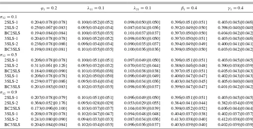
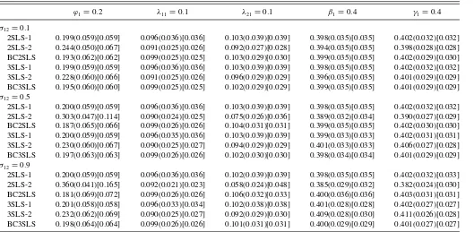
The estimation results of Equation (41) are reported in Tables 1–8. We report the mean and standard deviation (SD) of the empirical distributions of the estimates. To facilitate the com-parison of different estimators, we also report their root mean square errors (RMSE). The main observations from the experi-ment are summarized as follows.

(a) The additional IVs based on the numbers of friends in

Q2 reduce SDs of 2SLS and 3SLS estimators. When the IVs inQ1are strong (i.e.,β1=β2=γ1 =γ2=0.8 as in Tables 1–4) and the correlation across equations is weak (σ12=0.1), for the sample with nr=10 and

¯

r₌30 inTable 1, SD reductions of 2SLS-2 estimators of φ1, λ11, λ21, β1, γ1 (relative to 2SLS-1) are, respec-tively, about 3.9%, 17.1%, 14.7%, 1.5%, and 5.4%. As the correlation across equations increases, the SD re-duction also increases. Whenσ12=0.9 (see the bottom panel ofTable 1), SD reductions of 2SLS-2 estimators of

φ1, λ11, λ21, β1, γ1are, respectively, about 13.7%, 22.9%, 20.6%, 10.6%, and 10.9%. Furthermore, the SD reduc-tion is more significant when the IVs inQ1are less in-formative (i.e.,β1=β2=γ1=γ2=0.4 as in Tables5– 8). Whenσ12 =0.1 (see the top panel ofTable 5), SD reductions of 2SLS-2 estimators of φ1, λ11, λ21, β1, γ1 are, respectively, about 18.1%, 37.5%, 33.8%, 6.0%, and 12.3%. The SD reduction of the 3SLS estimator withQ2 follows a similar pattern.

(b) The additional IVs in Q2 introduce biases into 2SLS and 3SLS estimators. The size of the bias increases as the correlation across equationsσ12increases and as the IVs in Q1 becomes less informative (i.e., β1, β2, γ1, γ2 become smaller). The size of the bias reduces as the network size increases. The impact of the number of networks on the bias is less obvious.

(c) The proposed bias-correction procedure substantially re-duces the many-instrument bias for both the 2SLS and 3SLS estimators. For example, inTable 1, bias reductions of BC3SLS estimators ofφ1, λ11, λ21(relative to 3SLS-2) are, respectively, 100.0%, 100.0%, and 66.7%, when

σ12=0.1.

(d) The 3SLS estimator improves the efficiency upon the 2SLS estimator. The improvement is more prominent when the correlation across equations is strong. InTable 1, whenσ12 =0.9, SD reductions of BC3SLS estimators ofφ1, λ11, λ21, β1, γ1 (relative to BC2SLS) are, respec-tively, about 8.5%, 9.7%, 3.2%, 25.4%, and 14.5%.

(12)

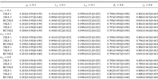
Table 1. 2SLS and 3SLS estimation (nr=10, r¯=30)

ϕ1=0.2 λ11=0.1 λ21=0.1 β1=0.8 γ1=0.8

σ12=0.1

2SLS-1 0.202(0.051)[0.051] 0.100(0.035)[0.035] 0.100(0.034)[0.034] 0.806(0.066)[0.067] 0.803(0.056)[0.056] 2SLS-2 0.223(0.049)[0.054] 0.093(0.029)[0.030] 0.095(0.029)[0.029] 0.799(0.065)[0.065] 0.802(0.053)[0.053] BC2SLS 0.198(0.055)[0.055] 0.100(0.030)[0.030] 0.101(0.030)[0.030] 0.806(0.066)[0.066] 0.803(0.054)[0.054] 3SLS-1 0.202(0.051)[0.051] 0.100(0.035)[0.035] 0.100(0.034)[0.034] 0.806(0.066)[0.066] 0.804(0.056)[0.056] 3SLS-2 0.216(0.053)[0.056] 0.093(0.029)[0.030] 0.097(0.030)[0.030] 0.800(0.065)[0.065] 0.805(0.053)[0.053] BC3SLS 0.200(0.054)[0.054] 0.100(0.030)[0.030] 0.101(0.030)[0.030] 0.806(0.066)[0.066] 0.803(0.054)[0.054]

σ12=0.5

σ12=0.9

NOTE: Mean(SD)[RMSE].

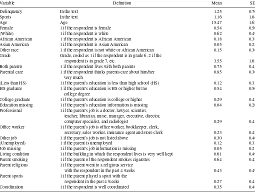
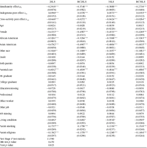
7. EMPIRICAL EXAMPLE

To illustrate the proposed estimators, we study the peer effect of sporting activities on juvenile delinquency using a unique and now widely used dataset provided by the National Lon-gitudinal Study of Adolescent Health (Add Health). The Add Health data provides national representative information on 7th– 12th graders in the United States. The in-school survey was

conducted during the 1994–1995 year with four follow-up in-home interviews. Here we only use the first wave of Add Health data.

In this empirical example, we consider the estimation of (29) and (30) whereY1 andY2are indices of participation in delin-quent conducts and sporting activities respectively. To be more specific, the Add Health survey reports the frequency of the

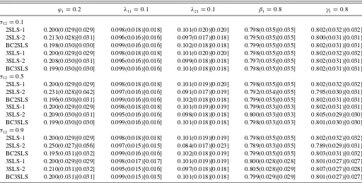
Table 2. 2SLS and 3SLS estimation (nr₌15, r¯₌30)

ϕ1=0.2 λ11=0.1 λ21=0.1 β1=0.8 γ1=0.8

σ12=0.1

σ12=0.5

σ12=0.9

(13)

Table 3. 2SLS and 3SLS estimation (nr =30, r¯=30)

ϕ1=0.2 λ11=0.1 λ21=0.1 β1=0.8 γ1=0.8

σ12=0.1

σ12=0.5

σ12=0.9

following delinquent behaviors in the past 12 months, namely, smoking cigarettes; drinking beer, wine, or liquor; getting drunk; racing on a bike, on a skateboard or roller blades, or in a boat or car; doing something dangerous due to dare; lying to parents or guardians; and skipping school without an excuse, coded us-ing an ordinal scale as 0 (never), 1 (once or twice), 2 (once

a month or less), 3 (2 or 3 days a month), 4 (once or twice a week), 5 (3–5 days a week), and 6 (nearly everyday).Y1 is given by the average frequency of the above delinquent behav-iors. In the sample considered, less than 5% of the students claimed they never committed the above delinquent conducts in the past 12 months.Y2corresponds to the average frequency of

Table 4. 2SLS and 3SLS estimation (nr ₌15, r¯₌60)

ϕ1=0.2 λ11=0.1 λ21=0.1 β1=0.8 γ1=0.8

σ12=0.1

σ12=0.5

σ12=0.9

(14)

ϕ1=0.2 λ11=0.1 λ21=0.1 β1=0.4 γ1=0.4

σ12=0.1

σ12=0.5

σ12=0.9

participating the following sporting activities in the past week, including going roller-blading, roller-skating, skate-boarding, or bicycling; playing an active sport, such as baseball, softball, basketball, soccer, swimming, or football; and doing exercise, such as jogging, walking, karate, jumping rope, gymnastics or dancing, coded as 0 (not at all), 1 (1 or 2 times), 2 (3 or 4 times), and 3 (5 or more times).

The adjacency matrixG₌[gij] is constructed based on the

friend-nomination information in the Add Health data. In the survey, the respondent is asked to nominate his/her best friends (up to 5 male friends and 5 female friends) from a school roster. Less than 1% of the students in the sample nominated 10 friends and thus the bound on the number of friend-nominations is not binding. We assume friendship is reciprocal. Thus, for students

ϕ1=0.2 λ11=0.1 λ21=0.1 β1=0.4 γ1=0.4

σ12=0.1

σ12=0.5

σ12=0.9

(15)

Table 7. 2SLS and 3SLS estimation (nr =30, r¯=30)

ϕ1=0.2 λ11=0.1 λ21=0.1 β1=0.4 γ1=0.4

σ12=0.1

σ12=0.5

σ12=0.9

Table 8. 2SLS and 3SLS estimation (nr ₌15, r¯₌60)

ϕ1=0.2 λ11=0.1 λ21=0.1 β1=0.4 γ1=0.4

σ12=0.1

σ12=0.5

σ12=0.9

iandj,gij =1 if eitherinominatesjorjnominatesias a friend

and gij =0 otherwise. After removing isolated students and

pairs (i.e., network with only two students), the sample consists of 8236 students distributed over 515 networks6_{, with network}

6_{Here, a network is defined as the largest set of students who are directly or}

indirectly connected through friend-nomination. By this definition, students from two different networks cannot be friends.

size ranging from 3 to 949. Because the strength of peer effect may vary with network sizes (Calv´o-Armengol, Patacchini, and Zenou 2009), we exclude networks larger than the 99th per-centile of the network size distribution. Our selected sample consists of 5,947 students distributed over 509 networks, with network sizes ranging from 3 to 140. The mean and the standard deviation of network size are 11.68 and 22.62. Furthermore, in our sample, the average number of friends of a student is 2.74