Full Terms & Conditions of access and use can be found at
http://www.tandfonline.com/action/journalInformation?journalCode=ubes20
Download by: [Universitas Maritim Raja Ali Haji] Date: 11 January 2016, At: 23:00
Journal of Business & Economic Statistics
ISSN: 0735-0015 (Print) 1537-2707 (Online) Journal homepage: http://www.tandfonline.com/loi/ubes20
Cointegration and Long-Run Asset Allocation
Ravi Bansal & Dana Kiku
To cite this article: Ravi Bansal & Dana Kiku (2011) Cointegration and Long-Run Asset Allocation, Journal of Business & Economic Statistics, 29:1, 161-173, DOI: 10.1198/ jbes.2010.08062
To link to this article: http://dx.doi.org/10.1198/jbes.2010.08062
Published online: 01 Jan 2012.
Submit your article to this journal
Article views: 168
Cointegration and Long-Run Asset Allocation
Ravi B
ANSALFuqua School of Business, Duke University, Durham, NC 27708 and NBER (ravi.bansal@duke.edu)
Dana K
IKUWharton School, University of Pennsylvania, Philadelphia, PA 19104 (kiku@wharton.upenn.edu)
We show that economic restrictions of cointegration between asset cash flows and aggregate consumption have important implications for return dynamics and optimal portfolio rules, particularly at long invest-ment horizons. When cash flows and consumption share a common stochastic trend (i.e., are cointegrated), temporary deviations between their levels forecast long-horizon dividend growth rates and returns, and consequently, alter the term profile of risks and expected returns. We show that the optimal asset allo-cation based on the error-correction vector autoregression (EC-VAR) specifiallo-cation can be quite different relative to a traditional VAR that ignores the cointegrating relation. Unlike the EC-VAR, the commonly used VAR approach to model expected returns focuses on short-run forecasts and can considerably miss on long-horizon return dynamics, and hence, the optimal portfolio mix in the presence of cointegration. We develop and implement methods to account for parameter uncertainty in the EC-VAR setup and high-light the importance of the error-correction channel for optimal portfolio decisions at various investment horizons.
KEY WORDS: Asset allocation; Cointegration; Long-run risks.
1. INTRODUCTION
Risks facing a short-run and long-run investor can be quite different. While at very short horizons, the contribution of cash-flow news to the variance of return may be small, as the in-vestment horizon increases, cash-flow fluctuations become the dominant source of return variability. Hence, understanding and modeling the behavior of asset returns, especially at long hori-zons, depend critically on understanding and modeling the dy-namics of their cash flows. In this article we argue that de-viations between cash-flow levels and aggregate consumption (the error-correction term) contain important information about means and variances of future cash-flow growth rates, and con-sequently, returns. Incorporating this cointegration restriction in return dynamics yields interesting implications for the term-structure of expected returns and risks, and hence, asset allo-cations at various investment horizons. In particular, we show that the error-correction mechanism significantly alters the risk-return tradeoff and the shape of optimal portfolio rules implied by models where the long-run adjustment of cash flows is ig-nored.
Our motivation for including the error-correction mechanism is based on the ideas of long-run risks developed inBansal and Yaron(2004),Hansen, Heaton, and Li(2005),Bansal, Dittmar, and Lundblad(2005), and Bansal, Dittmar, and Kiku(2009). These articles, both theoretically and empirically, highlight the importance of the long-run relation between cash flows and ag-gregate consumption for understanding the magnitude of the risk premium and its cross-sectional variation. Built on this ev-idence, our article aims to explore the effect of long-run prop-erties of asset cash flows on the optimal portfolio mix at var-ious investment horizons. Intuitively, if the long-run dynamics of asset dividends are described by a cointegrating relation with aggregate consumption, then current deviations between their levels should forecast future dividend growth rates (seeEngle and Granger 1987). Further, as risks in long-horizon returns are
dominated by cash-flow news, the predictability of asset divi-dends emanating from the error-correction mechanism may sig-nificantly alter the future dynamics of multihorizon returns and their volatilities. This suggests that the error-correction chan-nel may be very important for determining the optimal asset al-location at intermediate and long investment horizons. Earlier portfolio choice literature, including Kandel and Stambaugh (1996),Barberis(2000),Chan, Campbell, and Viceira(2003), andJurek and Viceira(2005), model asset returns via a standard vector-autoregression, and hence, ignore the consequences of the long-run dividend dynamics for the risk-return tradeoff and allocation decisions.
We measure the long-run relation between asset dividends and aggregate consumption via a stochastic cointegration. Based on the implications of the cointegrating relation, we model dividend growth rates, price-dividend ratios, and returns using an error-correction specification of a vector autoregres-sion (EC-VAR) model. Our time-series specification allows us to compute the term profile of conditional and unconditional means and the variance–covariance structure of asset returns, which we subsequently use to derive the optimal conditional and unconditional portfolio rules. To highlight the importance of the error-correction dynamics in dividends, we compare the resulting allocations with those impled by a standard VAR model, which excludes the error-correction variable from in-vestors’ information set.
We solve the portfolio choice problem for buy-and-hold mean-variance investors with different investment horizons, ranging from 1 to 15 years, and different levels of risk aver-sion. To emphasize the implications of long-run cash-flow dy-namics for the risk-return tradeoff and optimal portfolio mix, we focus on equities that are known to display large disper-sion in average returns and opposite long-run (cointegrating)
© 2011American Statistical Association Journal of Business & Economic Statistics
January 2011, Vol. 29, No. 1 DOI:10.1198/jbes.2010.08062
161
characteristics. In particular, we consider investors who allocate their wealth across value and growth (i.e., high and low book-to-market) stocks and the one-year Treasury bond. We distin-guish between conditional and unconditional portfolio choice problems and highlight the differences between the two.
To keep the analysis simple and transparent, we abstract from any types of dynamic rebalancing and focus on the first-order effect of the error-correction mechanism captured by the solu-tion to the mean-variance problem. As shown inJurek and Vi-ceira(2005), regardless of investors’ risk aversion, the intertem-poral hedging demand contributes a very small portion (less than 5%) to the variation of the overall portfolio weights across time. Thus, the volatility of the optimal portfolio is largely dominated by its myopic component, which our approach cap-tures. Considering reasonable alternative preference specifica-tions, while straightforward, is unlikely to materially alter our evidence.
We establish several interesting results. Consistent with Bansal, Dittmar, and Lundblad (2001),Hansen, Heaton, and Li (2005), and Bansal, Dittmar, and Kiku (2009), we find that value and growth stocks significantly differ in their ex-posures to long-run consumption risks. While cash flows of value firms respond positively to low-frequency consumption fluctuations, growth firms display a negative response in the long run. Importantly, we find that current deviations in the dividend-consumption pair (the cointegrating residual) contain distinct information about future dynamics of both cash flows and multihorizon returns, which is missing in the VAR setup. In particular, if the error-correction dynamics are ignored and returns are modeled via the standard VAR, one is able to ac-count for about 11% and 52% of the variation in growth and value returns at the 10-year horizon. With the cointegration-based specification, the long-run predictability of growth and value returns rises to striking 42% and 65%, respectively.
The forecasting ability of the error-correction term signifi-cantly alters variances (and covariances) of asset returns rel-ative to the growth rates-based VAR, especially at intermedi-ate and long horizons. As expected, the EC-VAR model gener-ates a declining pattern in the term structure of unconditional volatilities of both value and growth stocks. The standard de-viation of value returns in the VAR specification, on the other hand, is slightly increasing with the horizon. Hence, the EC-VAR model potentially is able to capture much larger benefits of time-diversification relative to the traditional VAR approach. Indeed, if the error-correction channel is ignored, the uncondi-tional allocation to value stocks steadily declines: the VAR in-vestors reduce their holdings of value stocks from 66% to about 52% as the investment horizon changes from 1 to 10 years. This pattern is consistent with the VAR-based evidence ofJurek and Viceira(2005). In contrast, relying on the cointegration-based specification, investors tend to allocate a much larger fraction of their wealth to value stocks as the investment horizon length-ens. In particular, the holding of value firms increases from 76% at the one-year horizon to about 96% for the 10-year invest-ment. Thus, optimal portfolio prescriptions based on the stan-dard VAR and EC-VAR models can be very different—these differences are a reflection of the error-correction mechanism between asset cash flows and aggregate consumption and the ensuing time-diversification effect. Given a strong economic
appeal of cointegration in dividend-consumption relation, our evidence suggests that investors should rely on the optimal port-folio mix based on the EC-VAR model.
It is well recognized in the literature that asset allocation de-cisions may be quite sensitive to parameter uncertainty. To en-sure that our results are robust to estimation errors, we sup-plement our evidence by deriving optimal allocations of a Bayesian-type investor who recognizes and accounts for uncer-tainty about model parameters. The impact of parameter un-certainty in a standard VAR framework was earlier analyzed in Kandel and Stambaugh(1996) andBarberis(2000). We extend their approach and develop a method that allows us to handle parameter uncertainty in the cointegration setup. We find the Bayesian-based evidence to be qualitatively similar to the no-uncertainty case. To be specific, even after accounting for un-certainty in model parameters, the EC-VAR and VAR specifi-cations deliver quite different portfolio rules, particularly in the intermediate and long run. As the horizon increases, the allo-cation to value continues to rise within the EC-VAR specifica-tion (from about 47% to 64% at the horizon extends from 1 to 10 years) and keeps on falling in the growth rates VAR framework (from 43% to 24%, respectively). Further, similar to Barberis(2000), we find that investors that doubt reliability of the estimated model parameters tend to shift their wealth away from equities toward safer securities. Depending on the hori-zon, the allocation to the Treasury bond increases by 20% to 40% compared to the no-uncertainty case. Taken together, our evidence suggests that parameter uncertainty affects the scale but not the shape of optimal asset allocations.
The rest of the article is structured as follows. Section2 de-scribes the evolution of risks across different investment hori-zons and points toward the importance of long-run dynamics of dividend growth rates for optimal decision rules. Section3 outlines the portfolio choice problem, highlights implications of cointegration, and describes the dynamic model for asset re-turns. Our empirical results and their discussion are presented in Section4. Finally, Section5concludes.
2. SOURCES OF RISKS AT DIFFERENT HORIZONS
Our motivation for incorporating long-run (cointegration) restrictions is the changing nature of risks across investment horizons. Although short and long-horizon investors are con-fronted by both risks in dividend growth rates and risks in price-dividend ratios, their concerns about the two are likely to be quite different since the relative contribution of dividend and price news to the overall return variation changes considerably with the horizon. While at short horizons, price risks are very important, their impact gradually diminishes due to stationar-ity of the price-dividend ratio. Consequently, at long investment horizons, variation in returns is dominated by risks in dividends. To formalize this intuition, we perform a variance decom-position of returns using a first-order VAR model for dividend growth rates and log price-dividend ratios. Specifically, we project dividend growth of an asset on its own lag and regress the price-dividend ratio on one lag of the dividend growth, as well as its own lag. To provide a clean interpretation of the role of price shocks versus dividend shocks we orthogonalize the VAR innovations by assuming that dividend news leads to price
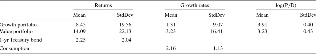
Table 1. Data summary
Returns Growth rates log(P/D)
Mean StdDev Mean StdDev Mean StdDev
Growth portfolio 8.45 19.56 1.31 9.07 3.91 0.40 Value portfolio 14.09 22.13 3.23 16.41 3.23 0.43
1-yr Treasury bond 2.25 2.04
Consumption 2.16 1.13
NOTE: This table presents descriptive statistics for returns, dividend growth rates and logarithms of price/dividend ratios of value and growth firms, the return on the one-year Treasury bond and consumption growth. Value firms represent companies in the highest book-to-market quintile of all NYSE, AMEX, and NASDAQ firms. Growth firms correspond to the lowest book-to-market quintile. Portfolios are constructed as inFama and French(1993). Returns are value-weighted, price/dividend ratios are constructed by dividing the end-of-year price by the annual per-share dividend, growth rates are constructed by taking the first difference of the logarithm of per-share dividend series. Time-series for the Treasury bond are taken from the CRSP Fama-Bliss Discount Bonds files. Data on the per-capita consumption of nondurables and services come from the NIPA tables available from the Bureau of Economic Analysis. All data are sampled on at the annual frequency, converted to real using personal consumption deflator, and cover the period from 1954 to 2003.
movements, but price innovations do not lead to contempora-neous responses in dividends. We implement variance decom-position for two equity portfolios: growth and value stocks that we subsequently use in our asset allocation analysis. Growth and value stocks represent the lowest and the highest quintile of book-to-market sorted portfolios, respectively. The construc-tion of portfolios and their dynamics are presented in Table1.
We find that the contribution of dividends and price-dividend ratios to return variation changes significantly with the hori-zon. In the short run, price risks dominate—for both portfo-lios, about 98% of return variation over the one-year horizon is attributed to price news. However, as the holding interval in-creases, risks in returns shift toward risks in dividends. By the 10-year horizon, more than half of return variation is due to div-idend shocks. As the horizon reaches 20 years, divdiv-idend growth risks account for 75% of variation in growth returns and more that 90% of risks in value returns. This evidence suggests that asset allocations at long investment horizons are mostly about managing dividend risks. Thus, understanding low-frequency dynamics of asset dividends and integrating them into a model for the risk-return tradeoff is critical in designing optimal al-locations for long-horizon investors. In this article, we model the dynamics of asset dividends via a cointegrating relation with aggregate consumption and show that the ensuing error-correction channel has important implications for optimal port-folio rules at intermediate and long investment horizons. In the next section, we set out the portfolio choice problem and de-scribe the dynamics of asset returns that account for long-run consumption risks in dividends.
3. ASSET ALLOCATION FRAMEWORK
3.1 Portfolio Choice Problem
We consider investors with constant relative risk aversion preferences (CRRA) preferences who follow a buy-and-hold strategy over different holding horizons. At timet, an investor chooses an allocation that maximizes her expected end-of-period utility and is locked into the chosen portfolio till the end of her investment horizon. Specifically, the s-period investor solves
max
αs,t
Et[Ut+s] =max
αs,t
Et W1−γ
t+s 1−γ
, (1)
whereαs,t is the vector of portfolio weights, Wt+s is the ter-minal wealth, and γ is the coefficient of risk aversion (RA). LettingRpt+1→t+sdenote the (gross) return on the portfolio held by the investor,
Rpt+1→t+s=αs′,tRt+1→t+s, (2) whereRt+1→t+sis the vector of compounded asset returns, the evolution of wealth is described by
Wt+s=Wt∗Rpt+1→t+s. (3) We distinguish between the conditional and unconditional stock allocation problems. The conditional problem is stated above and uses the conditional distribution of future returns. The un-conditional asset allocation relies on the unun-conditional distrib-ution of asset returns to maximize expected utility.
To make the problem tractable, we will assume throughout that gross asset returns are lognormally distributed. As shown inCampbell and Viceira(2002), the investor’ objective function in this case can be written as
max αs,t
Et[r p
t+1→t+s] + 1 2Vart(r
p t+1→t+s)
−γ
2 Vart(r p t+1→t+s)
, (4)
whererpt+1→t+sis the log return on a portfolio bought at timet
and held up tot+s. The unconditional problem can be restated analogously by dropping the time subscripts in the expression above. We will refer toEt[rpt+1→t+s]as the expected log return andEt[rtp+1→t+s] +
1 2Vart(r
p
t+1→t+s)as the arithmetic mean re-turn. In the empirical section, the reported mean returns corre-spond to arithmetic means. To enhance the comparison across different holding periods, we measure and express all asset re-turn moments per unit of time, that is, we scale both means and variances by the investment horizon.
There are three assets available to investors: in addition to the one-year Treasury bond, they allocate their wealth between growth and value stocks. We focus on stocks with opposite book-to-market characteristics that, historically, are known to display large dispersion in average returns (as shown in Ta-ble1). The data employed in our empirical work are sampled on the annual frequency, thus, a single investment period corre-sponds to one year. We set risk aversion at five in our bench-mark case; in addition, we highlight the implications of in-vestors’ preferences by entertaining a higher risk aversion level of 10.
3.2 Modeling Asset Returns
3.2.1 Cointegration Specification. We describe the long-run dynamics of dividends and consumption via a cointegrating relation,
dt=τ0+τ1t+δct+ǫd,t, (5) wheredt is the log level of an asset’s dividend, ct is the log level of aggregate consumption, andǫd,t ∼I(0)is the cointe-grating residual or the error-correction term. It follows from Equation (5) that dividend growth evolves asdt≡τ1+δct+ ǫd,t. Hence, a time-series model forǫd,t andctis sufficient to model the dynamics of cash-flow growth rates.
Our specification implies that dividends and consumption share a common stochastic trend. The two, however, may ex-hibit different exposures to the underlying long-run risks as we do not impose a unit restriction on the cointegration parame-ter,δ. In addition, by including the time-trend in Equation (5), we allow for differences in deterministic trends in asset divi-dends and aggregate consumption. As we argue, imposing re-strictions on eitherτ or δmay not be appropriate for the divi-dend series we rely on.
Following the existing asset pricing literature, we focus on dividends constructed on the per-share basis. These dividends correspond to a trading strategy of holding one share of a firm’s stock at each point in time. An investor following the one-share strategy will consume all the dividends and reinvests only cap-ital gains. Consider, alternatively, an investor who plows a por-tion of the received cash back into the firm. If the amount of reinvested income matches the net share issuance, such an in-vestor will hold a claim to the total equity capital of the firm. Consequently, payout series associated with this alternative in-vestment, which we refer to as aggregate dividends, are propor-tional to the firm’s market capitalization. Notice the difference between the two measures—while the per-share series account for the growth of the share price, aggregate dividends reflect the appreciation of the firm’s equity capital.
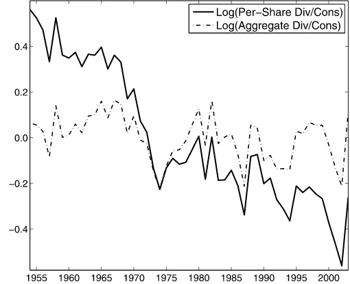
It may be theoretically appealing to omit the time trend and restrict the cointegration parameter of aggregate dividends on the market (or a particular sector of the economy) to one, as it will yield balanced growth paths of aggregate payouts and ag-gregate consumption. There is, however, no economic rationale for such restrictions for dividends per share. In order to illus-trate and reinforce this important point, Figure1plots the log of the stock market dividend to consumption ratio for the two dividend measures. While the ratio of aggregate dividends to consumption appear to be stationary, the ratio of per-share div-idends to consumption displays a dramatic decline over time. The reason per-share dividends fail to catch up with the level of aggregate consumption is due to the fact that per-share se-ries, by construction, do not account for capital inflow in equity markets.Bansal and Yaron(2006) provided further discussion of the difference between the two trading strategies and implied dividend series.
From an econometric perspective, the distinction between aggregate and per-share dividends has important implications for modeling the dynamics of asset returns. As Figure1shows, per-share dividends and aggregate consumption tend to drift apart over time and the cointegrating relation between the two
Figure 1. Dividend to consumption ratio. This figure plots the logarithm of per-share dividends to aggregate consumption ratio (solid line), and the log ratio of aggregate dividends to consumption (dash-dotted line). Dividend series represent cash flows of the aggre-gate stock market portfolio. Per-share dividend series are constructed asDt+1=Yt+1Pt, whereYandPare the dividend yield and the price
index respectively; the latter evolves according toPt+1=Ht+1Pt,P0 is normalized to 1, andHis the price gain. Aggregate dividend series are constructed asDaggt+1=Yt+1Kt, whereKis the market
capitaliza-tion. The data are real and span the period from 1954 to 2003.
cannot be established under the{δ=1 &τ =0}restriction as confirmed by the augmented Dickey–Fuller test. Hence, omit-ting the time trend and imposing the{δ=1 &τ =0} restric-tion in the data leads to explosive/nonstarestric-tionary return dynam-ics. This issue is also discussed inBansal, Dittmar, and Kiku (2009).
The asset pricing literature typically focuses on the per-share dividends as their present value corresponds to the price of the asset, which is not true for aggregate dividend series. We follow this tradition and use series constructed on the per-share basis. Given the earlier discussion, we do not impose any restrictions on parameters that govern their long-run dynamics, letting the data decide on the underlying cointegrating relation between per-share dividends and aggregate consumption.
3.2.2 Return Dynamics. To describe the distribution of asset returns at various investment horizons, we model the dy-namics of single-period returns and state variables jointly via the following EC-VAR,
That is, we project log bond return, bt, and consumption growth, ct, on their own lags, and regress the
ing residual,ǫd,t, log price-dividend ratio,zt, and log return,
rt, on their lags (excluding lagged return) and past consump-tion growth. DenotingX′t=(bt ct ǫd,t zt rt), we can rewrite the EC-VAR in a compact matrix form,
Xt+1=a+AXt+ut+1, (7)
whereais the vector of intercepts, the matrixAis defined ear-lier, anduis a(5×1)-matrix of shocks that follow a normal dis-tribution with zero mean and variance–covariance matrixu. For expositional purposes, we focus of the first-order EC-VAR. It is easy to allow for higher-order dynamics as they always can be mapped into the first-order representation.
The error-correction specification is the key dimension that differentiates our article from the existing portfolio choice lit-erature. The latter typically models asset returns via a simple VAR that incorporates information on the price-dividend ratio (seeKandel and Stambaugh 1996;Barberis 2000;Chan, Camp-bell, and Viceira 2003; andJurek and Viceira 2005among oth-ers). In contrast to the traditional VAR approach, we describe the dynamics of asset returns using the error-correction frame-work that exploits the implications of long-run relation between dividends and consumption.
The conceptual difference between a standard VAR and the EC-VAR specifications is summarized by the error-correction variable,ǫd,t. To see its implications for returns consider a Tay-lor series approximation of log returns (as in Campbell and Shiller 1988),
rt+1=κ0+dt+1+κ1zt+1−zt, (8) whereκ’s are constants of linearization. As long-horizon re-turns can be computed via summing up both sides of Equa-tion (8), multiperiod returns will depend on the dynamics of long-horizon dividend growth rates. Thus, long-run predictable variation in dividend growth via the cointegrating residual (Engle and Granger 1987) might alter predictability, and hence, distribution of multiperiod returns. In fact, cointegration be-tween dividends and consumption has potentially the same eco-nomic consequences for returns as the unit cointegration restric-tion between prices and dividends. While price-dividend ratios are commonly used to forecast long-horizon returns, we argue that the error-correction residual, ǫd,t, may be equally (if not more) important for predicting future returns; as such, it may significantly affect volatilities and correlations of multiperiod returns. Consequently, including the error-correction variable in the return dynamics may alter our views of the optimal long-run allocations.
To highlight the importance of the error-correction mech-anism in cash flows for the risk-return tradeoff and optimal portfolio decisions, we will compare the implications of the cointegration-based EC-VAR to those implied by the tradi-tional VAR specification. In the VAR setup, the error correction variable in Equation (6),ǫd,t, is simply replaced by dividend growth,dt.
Notice that instead of estimating the dynamics of asset re-turns directly as in Equation (6), one can infer them from the joint dynamics of price-dividend ratio and dividend growth according to the log-linear approximation in Equation (8). As shown inCampbell and Shiller(1988), the approximation works well at relatively short investment horizons. However,
once compounded, the approximation error can lead to sizable distortions in multihorizon return moments, and hence, long-horizon asset allocations. Quantitatively, we find that at hori-zons of 10 to 15 years, the volatility of approximate returns is likely to over or understate the true return volatility by 2% to 4%, or 15% to 20% in relative terms (see theAppendixfor details). Although our empirical evidence will not materially change if we rely on log-linearization of asset returns, by mod-eling the dynamics of asset returns explicitly we are able to purge the effect of log-linearization and derive allocations that are not subject to the approximation error.
3.3 Term Structure of Expected Returns and Risks
The solution to the portfolio choice problem in Equation (4) hinges on the distribution of multiperiod returns, in particular, its first two moments. The required term-profile of expected re-turns and risks can be easily computed by exploiting the recur-sive structure of the EC-VAR as we outline in the following.
3.3.1 Unconditional Analysis. The solution to the uncon-ditional problem is derived by fixing expected log returns on individual assets at their sample means, i.e.,
E[rt+1→t+s] =
To compute the unconditional variance of asset returns at vari-ous investment horizons, we exploit the stationarity property of EC-VAR variables and present the original specification as an infinite-order moving average,
It follows, then, that the unconditional variance ofXtis
∗0=
and the variance of the sum ofsconsecutiveX’s is given by
∗s=s0+
s , the unconditional vari-ance of multiperiod returns (expressed per-unit time) can be ex-tracted via,
Var(rt+1→t+s)=ι′rsιr, (13) where ιr is a (5×1)-indicator vector with the last element (corresponding to return) set equal to 1. As pointed out ear-lier, while the expected log returns E[rt+1→t+s] are constant across horizons, the unconditional variances may change with the horizon. Thus, although the unconditional problem does not accommodate market timing, it does exploit return predictabil-ity via horizon-dependent variances and correlations.
3.3.2 Conditional Analysis. In the conditional problem, we rely on the above EC-VAR to measure both expected values and variance–covariance structure of asset returns. Specifically, the mean of the continuously compounded return is computed as
for a given horizons≥1, the innovation in the sum ofs con-secutiveX’s can be extracted as follows:
s
Exploiting the fact that errors are identically distributed and se-rially uncorrelated, the covariance matrix ofζt,t+sfor any given horizonsis
s , that is, the covariance ma-trix ofζt,t+sscaled by the horizon. GivenuandGs, the
evo-The term structure of risks in returns can now be extracted by taking the corresponding element of thes-horizon matrix,
Vart(rt+1→t+s)=ι′rsιr. (17) The arithmetic mean return can be constructed by adding half the variance to the expected log return given by Equation (14). The covariance between assets returns is calculated by stack-ing individual EC-VAR models and applystack-ing the same recursive procedure to the augmented system.
The solution to the conditional problem incorporates both horizon and time dimensions, allowing us to trace the impact of time-diversification as well as time-varying economic con-ditions on optimal allocations. Investors, in this case, are said to time the market by choosing their portfolios according to the current level of state variables.
3.4 Incorporating Parameter Uncertainty
Despite the growing evidence of time-variation in expected returns, it is well recognized that the true predictability of asset returns is highly uncertain. Furthermore, the predictive power of popular forecasting instruments, such as dividend yields, price-earning ratios or interest rates, is highly unstable across sample periods and sampling frequencies (Stambaugh 1999; Goyal and Welch 2003). This may raise concerns as to what
extent investors incorporate the data evidence on return pre-dictability in their investment decisions. We address this is-sue in a Bayesian framework similar toKandel and Stambaugh (1996) andBarberis(2000).
The difference between a frequentist and a Bayesian ap-proaches lies in the probability distribution of asset returns that they rely on. In the former case, the term-structure of the risk-return relation is measured using the distribution conditioned on both the data and the point estimates. The Bayesian analysis, on the other hand, relies on the so-called predictive distribution of future returns conditioned only on the observed sample. To in-tegrate out parameter uncertainty we use the standard Bayesian technique summarized in theAppendix.
Our analysis differs fromKandel and Stambaugh(1996) and Barberis(2000) as they designed optimal allocations using the standard VAR approach, and thus, do not entertain parameter uncertainty emanating from estimating cointegration parame-ters. Incorporating uncertainty in our EC-VAR setup leads to two layers of estimation risk. The first is induced by the un-certainty in the cointegrating relation, the second arises from the uncertainty about the EC-VAR parameters. Following the literature, we impose a flat prior on the EC-VAR model para-meters, but consider an informative prior on the cointegrating relation between asset dividends and aggregate consumption. In particular, we assume that the prior distribution of the coin-tegration parameter is normal and centered at 1. To highlight the sensitivity of optimal asset allocations to prior uncertainty about the cointegration parameter, we allow for various degrees of invertors’ confidence. In the first case, which we refer to as the “tight” prior, we assume that 95% of the probability mass of the distribution of the cointegration parameter lies in the 0.5 to 1.5 range. In the second, “loose” prior case, we expand the confidence interval from −1 to 3. In the case of the standard VAR we assume a noninformative prior.
4. EMPIRICAL RESULTS
4.1 Return Dynamics
In this section we discuss the dynamics of the state vari-ables and returns across various investment horizons implied by our EC-VAR specification. Our benchmark results are based on parsimonious first-order dynamics. We subsequently highlight the robustness of our evidence to the inclusion of higher-order terms. We start by presenting empirical evidence on cointegra-tion and analyzing the ability of the error-correccointegra-tion variable to predict future dividend growth rates and returns. Our con-sumption and financial data are standard and described in the footnote to Table1.
4.1.1 Cointegration Evidence. We estimate cointegration parameters via ordinary least squares (OLS) by regressing log dividends on log consumption and a time trend. For both growth and value stocks, the sample autocorrelations of the resulting cointegrating residuals exhibit a rapid decline, from about 0.8 at the first lag to around−0.2 at the fifth lag. Formally, the aug-mented Dickey–Fuller test rejects the unit root null in the error-correction term at the 5% level for growth stocks and about 10% to 15% for value portfolio. This supports our assumption that the dynamics of the portfolios’ dividends and aggregate consumption are tied together in the long run.
Long-run risk properties of value and growth firms, however, are very different. While cash flows of value firms respond pos-itively to persistent shocks in aggregate consumption, growth firms’ dividends exhibit an opposite, negative exposure to low-frequency consumption fluctuations. In particular, the parame-ter of cointegration is estimated at 1.94 (SE=2.30) for high book-to-market firms and −4.84 (SE =0.97) for low book-to-market firms. Similar estimates are obtained in the dynamic OLS framework ofStock and Watson(1993). The dynamic or-dinary least squares (DOLS) estimate of the long-run exposure of asset dividends to consumption is equal to 1.58 (SE=2.11) and−5.41 (SE =1.01) for value and growth stocks, respec-tively. Our evidence is consistent with the cross-sectional pat-tern in long-run dividend betas documented inBansal, Dittmar, and Lundblad (2001), Hansen, Heaton, and Li (2005), and Bansal, Dittmar, and Kiku(2009).
The implications of cointegration for future growth rates can intuitively be explained via the error-correction mechanism. Assume that dividends are unusually high today. Since the coin-tegrating residual is stationary, dividend growth rates are ex-pected to fall since dividends have to adjust back to their long-run equilibrium with consumption. Thus, variation in future dividend growth rates should be accounted for by variation in the error-correction variable. Further, the slower the adjustment of dividends to the consumption level, the longer the effect of the cointegrating residual on future growth rates. Given that dividend growth is a key input in thinking about multihorizon returns, predictability of dividends emanating from the coin-tegrating relation may have important consequences for pre-dictability and volatility of future returns.
4.1.2 Predictability Evidence. In this section, we exam-ine the ability of the cointegrating residual to forecast asset re-turns at various horizons. To highlight the importance of the cointegrating relation, we compareR2’s for return projections implied by the EC-VAR model with the corresponding R2’s from the growth-rates-based VAR. The predictive state vari-ables in the EC-VAR are consumption growth, price-dividend ratio, and cointegrating residual of the asset. In the VAR speci-fication, we replace the asset’s error-correction term (ǫd,t) with dividend growth (dt). Hence, in both cases we have three vari-ables that forecast future equity returns. Note that we do not in-corporate past prices and dividends of one asset when describ-ing the dynamics of the other asset return as those brdescrib-ing vir-tually no additional predictive information. Statistically, once asset’s own lagged attributes are included, the other asset does not improve the predictive capacity of the forecasting regres-sions.
Table2presentsR2’s implied by the EC-VAR and the alterna-tive, growth rates model. As inHodrick(1992), long-horizons
R2’s are calculated as one minus the ratio of the innovation vari-ance in the return compounded over a given horizon sto the total variance ofs-period returns, i.e.,
R2s=1−ι
′ rsιr
ι′ rsιr
, (18)
wheresandsare defined previously. The numbers reported in parentheses are the 2.5% and 97.5% percentiles of the cor-responding bootstrap distributions. First, notice that return pre-dictability implied by our EC-VAR specification improves con-siderably with the horizon. As Panel A shows, the EC-VAR
Table 2. Return predictability
Horizon Growth Value
Panel A: Error-correction VAR
1 0.12 (0.07, 0.33) 0.17 (0.10, 0.39) 2 0.16 (0.11, 0.39) 0.26 (0.17, 0.45) 5 0.28 (0.17, 0.52) 0.46 (0.31, 0.62) 10 0.42 (0.22, 0.58) 0.65 (0.43, 0.73) 15 0.48 (0.23, 0.61) 0.73 (0.43, 0.79)
Panel B: Growth-rates VAR
1 0.11 (0.07, 0.43) 0.18 (0.11, 0.44) 2 0.12 (0.07, 0.46) 0.27 (0.15, 0.57) 5 0.12 (0.05, 0.51) 0.45 (0.19, 0.75) 10 0.11 (0.03, 0.51) 0.52 (0.13, 0.70) 15 0.10 (0.02, 0.50) 0.47 (0.10, 0.60)
NOTE: This table presents returnR2’s implied by the EC-VAR specification (Panel A) and the alternative growth rates-based VAR model (Panel B). The latter ignores the implica-tions of cointegration between asset cash flows and consumption. The entries are reported for value and growth portfolios across various holding horizons. Numbers in parentheses are the lower and upper bounds of the corresponding 95% bootstrap confidence intervals.
model accounts for only about 12% to 17% of the one-period return variation. However, by the 10-year horizon its predictive ability increases to striking 42% and 65% for growth and value stocks, respectively. Second, while none of the models seems to outperform the other in the short run, the growth rates VAR is noticeably dominated by the error-correction specification at longer horizons. This evidence suggests that the cointegrating residual incorporated in the EC-VAR specification contains dis-tinct and important information about return dynamics, espe-cially in the long run. To ensure robustness, we also considered direct projections of multiperiod returns on the EC-VAR and VAR predictive variables. TheR2’s from these regressions are very similar to those reported in Table2.
As discussed earlier, dividend risks are an important com-ponent of return variation, especially at long horizons. Thus, predictability of multihorizon returns is largely driven by pre-dictability of cash-flow growth rates. In the presence of cointe-gration, the error-correction specification should forecast div-idend risks much better than the standard VAR. Indeed, we find a sizable improvement in predicting long-horizon dividend growth rates with the EC-VAR model. For example, in the VAR specification, the adjusted R2 for predicting dividend growth rates at the five year horizon is about 22% for growth, and only 4% for value firms. In the EC-VAR, the corresponding numbers increase to 39% for growth and 18% for value stocks.
4.1.3 Term Profile of Means and Variances. Our pre-dictability evidence suggests that the error-correction mecha-nism may have an important bearing on the evolution of the expected return-risk relation across investment horizons, which we now explore in details. The profile of arithmetic means and unconditional volatilities of asset returns is presented in Table3. To emphasize the differences between the EC-VAR and the al-ternative VAR setup we display return moments for both mod-els. As Panel A shows, the term structure of arithmetic mean returns on low and high book-to-market firms is declining with the horizon for the EC-VAR specification. In contrast, there is almost no decline in mean returns of value stocks in the VAR
Table 3. Term structure of expected returns and risks
Expected return Volatility
Horizon Growth Value Bond Growth Value Bond
Panel A: Error-correction VAR
1 0.082 (0.014) 0.133 (0.019) 0.022 (0.000) 0.186 (0.019) 0.203 (0.021) 0.000 (0.000) 2 0.081 (0.014) 0.131 (0.019) 0.022 (0.005) 0.181 (0.017) 0.193 (0.019) 0.022 (0.004) 5 0.078 (0.014) 0.128 (0.019) 0.023 (0.006) 0.168 (0.018) 0.175 (0.023) 0.030 (0.006) 10 0.076 (0.014) 0.126 (0.020) 0.023 (0.006) 0.153 (0.020) 0.161 (0.030) 0.034 (0.007) 15 0.074 (0.014) 0.125 (0.021) 0.023 (0.006) 0.141 (0.021) 0.155 (0.035) 0.036 (0.008)
Panel B: Growth-rates VAR
1 0.080 (0.023) 0.132 (0.029) 0.022 (0.000) 0.179 (0.017) 0.198 (0.021) 0.000 (0.000) 2 0.080 (0.023) 0.132 (0.029) 0.022 (0.005) 0.176 (0.017) 0.195 (0.020) 0.022 (0.004) 5 0.078 (0.024) 0.132 (0.031) 0.023 (0.006) 0.168 (0.021) 0.195 (0.026) 0.030 (0.006) 10 0.077 (0.025) 0.133 (0.033) 0.023 (0.006) 0.159 (0.027) 0.199 (0.037) 0.034 (0.007) 15 0.076 (0.026) 0.133 (0.034) 0.023 (0.006) 0.153 (0.031) 0.203 (0.042) 0.036 (0.008)
NOTE: This table reports the profile of mean returns and volatilities by horizon. Expected returns and risks are presented for the EC-VAR specification (Panel A) and the alternative growth rates-based VAR model (Panel B). The latter ignores the implications of cointegration between asset cash flows and consumption. Bootstrap standard errors are reported in parentheses.
specification (see Panel B). Recall that in the unconditional case, the arithmetic mean return for a given horizon is defined as the mean log return plus one-half of the scaled variance of the multihorizon return. Clearly, the first component is the same in both the EC-VAR and VAR specifications, as it is simply de-termined by the historical average of log asset returns. The vari-ance component, however, depends on the time-series dynam-ics and predictability of long-horizon returns, and consequently, may significantly differ between the competing models.
Indeed, we find that volatilities of asset returns at vari-ous horizons are quite different across the two specifications. As expected, the standard deviation of long-run returns is re-duced within the error-correction framework for both value and growth stocks. The volatility of returns implied by the alter-native VAR specification similarly decreases for growth firms, but displays a generally flat (slightly increasing) pattern for value firms. In particular, the standard deviation of value re-turns declines from 20% at the one-year horizon to about 15% at the long horizon for the EC-VAR specification, but stays at the initial 20% for the VAR model. Thus, the EC-VAR spec-ification captures considerable time-diversspec-ification benefits in value returns that are overlooked by the VAR model.
Differences between the error-correction and growth rates specifications are pronounced not only for volatilities but also correlations of asset returns. In particular, in the EC-VAR the correlations of returns are much higher than in the VAR model. In the latter setup, the correlations decline from 0.63 to about 0.30 from the one to 15-year horizon. In contrast, for the EC-VAR, the correlation starts at 0.75 and gradually decreases to about 0.52. We should emphasize that these differences are not solely driven by the differences in returns’ variances across the two models—the EC-VAR and VAR-implied covariances like-wise significantly deviate from each other. This evidence im-plies that from the VAR perspective, diversification across as-sets can be quite important—growth asset can be valuable at long horizons despite its lower mean for purposes of reduc-ing the overall volatility of the optimal portfolio. The cross-sectional diversification seems to be less valuable from the EC-VAR perspective.
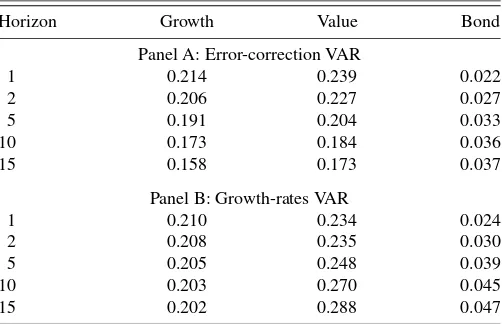
To investigate the impact of the estimation error on return moments, in Table4we report return volatilities after account-ing for parameter uncertainty. Mean returns are not reported for brevity—across all horizons, they are about 1% lower than their counterparts in the case when parameter uncertainty is ignored. Not surprisingly, the volatility of asset returns is higher when estimation errors are taken into account. However, the general pattern is similar to the case when parameter uncertainty is ig-nored.
To summarize, the empirical evidence presented in this sec-tion underscores the importance of the cointegrasec-tion specifica-tion for risks and expected returns. Temporary deviaspecifica-tions of cash flows from the permanent component in consumption con-tain important information about future dynamics of asset re-turns, and consequently, the term structure of the risk-return tradeoff. Furthermore, cointegration alters risk diversification properties of value and growth assets relative to the standard VAR model that, we expect, may significantly affect wealth al-location across the two stocks.
Table 4. Term structure of return volatilities with parameter uncertainty
Horizon Growth Value Bond
Panel A: Error-correction VAR
1 0.214 0.239 0.022 2 0.206 0.227 0.027 5 0.191 0.204 0.033 10 0.173 0.184 0.036 15 0.158 0.173 0.037
Panel B: Growth-rates VAR
1 0.210 0.234 0.024 2 0.208 0.235 0.030 5 0.205 0.248 0.039 10 0.203 0.270 0.045 15 0.202 0.288 0.047
NOTE: This table reports standard deviations of the predictive distribution of multi-period returns. The term profile of asset risks is presented for the EC-VAR specification (Panel A) and the alternative growth rates-based VAR model (Panel B). Panel A is con-structed imposing “tight” prior on the cointegration vector, centered around one.
4.2 Asset Allocation Decisions
Using the profile of constructed return moments, we solve for the optimal allocations of investors with different holding inter-vals. For brevity, in the benchmark case of no-parameter uncer-tainty, we report allocations for the risk aversion level of 5. The impact of investors’ preferences is illustrated later on, for the case that incorporates estimation uncertainty in model parame-ters. In there we consider two values of risk aversion, 5 and 10, and two levels of prior confidence, “loose” and “tight,” defined earlier. For simplicity, we ignore short selling constraints; the essential message is similar if one were to impose these restric-tions.
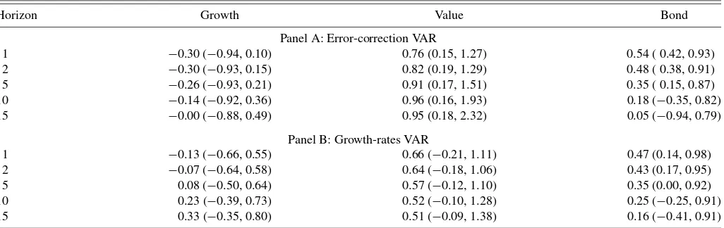
4.2.1 Unconditional Analysis. Asset allocations of the EC-VAR-based investors are reported in Panel A of Table5. We find that their investment strategy is considerably tilted to-ward value stocks at both short and long horizons. In particular, the allocation to value firms starts at about 76% at the one-year horizon, increasing to 95% at the 15-year horizon. The allo-cation to growth increases as well but it starts with a negative position. In addition, the level of growth investment is signifi-cantly lower than the allocation to value stocks at any horizon.
The horizon effect has an opposite pattern for the alternative VAR specification, as suggested by the entries in Panel B. At the very short horizon, the VAR-based investors still allocate more to value than to growth stocks. Their preferences toward the two assets, however, reverse as the holding period lengthens— as the horizon increases, the allocation to value declines and that to growth increases. This is consistent with the evidence inJurek and Viceira(2005). In a similar VAR setup, they also found that long-run investors gradually shift their wealth away from value stocks.
The documented differences in the optimal portfolio mix across the two models arise due to different patterns in return volatilities and their correlations. The VAR-based investors per-ceive value stocks as quite risky, especially in the long run, thus, steadily reducing their allocations to high book-to-market firms. In contrast, the EC-VAR investors recognize that, via the error-correction mechanism, the relative riskiness of value in-vestment shrinks over time. At short horizons, transitory risks in
dividends and prices make value stocks look quite risky. In the long run, transitory fluctuations are washed away and all risks in value returns come from permanent risks in their dividends. Im-portantly, the adjustment of value dividends, and thus, value re-turns to their long-run equilibrium relation with aggregate con-sumption is strongly predicted by the error-correction variable. This long-run predictability reduces the volatility of multihori-zon returns making value firms more attractive for long-horimultihori-zon investments. Further, while in the VAR, the cross-sectional di-versification via growth returns increases, its benefits are sig-nificantly reduced in the cointegration-based framework. Thus, the EC-VAR-based investors do not view growth stocks as good substitutes for value.
We find that across all horizons, investors are better off by following the cointegration-based allocation strategy rather than that prescribed by the standard VAR. Utility gain asso-ciated with the EC-VAR specification is increasing with the horizon when predictability coming from the error-correction mechanism takes stronger effect. For example, at the one-year investment horizon, the EC-VAR and VAR specifications yield about 0.050 and 0.049 utilities, respectively. By the five-year horizon, the difference in utilities is about 20%. At the 15-year horizon, the error-correction implied utility is about 0.065, while the VAR-based allocation guarantees only about 0.050, which amounts to more than 30% difference.
Our evidence is quite robust with respect to the order of the EC-VAR and VAR dynamics. We find that across various plau-sible specifications, allocation to value stocks is always increas-ing with the horizon in the error-correction case and always declining in the growth rates-based VAR. For example, the EC-VAR(2)-based investor will choose to increase her holdings of value stocks from 0.70 to about 1.04 as the horizon increases from one to five years. Investors that follow VAR(2) strategy, on the other hand, will choose to allocate about 53% of their wealth to value stocks at the one-year horizon, and about 48% at the five-year horizon. Higher-order specifications, as well, do not change the documented patterns in asset allocations and do not alter the magnitudes of portfolio weights in any economi-cally meaningful way.
We now turn the discussion to the portfolio choice in the presence of parameter uncertainty, which is reported in Table6.
Table 5. Optimal allocation strategy
Horizon Growth Value Bond
Panel A: Error-correction VAR
1 −0.30 (−0.94, 0.10) 0.76 (0.15, 1.27) 0.54 ( 0.42, 0.93) 2 −0.30 (−0.93, 0.15) 0.82 (0.19, 1.29) 0.48 ( 0.38, 0.91) 5 −0.26 (−0.93, 0.21) 0.91 (0.17, 1.51) 0.35 ( 0.15, 0.87) 10 −0.14 (−0.92, 0.36) 0.96 (0.16, 1.93) 0.18 (−0.35, 0.82) 15 −0.00 (−0.88, 0.49) 0.95 (0.18, 2.32) 0.05 (−0.94, 0.79)
Panel B: Growth-rates VAR
1 −0.13 (−0.66, 0.55) 0.66 (−0.21, 1.11) 0.47 (0.14, 0.98) 2 −0.07 (−0.64, 0.58) 0.64 (−0.18, 1.06) 0.43 (0.17, 0.95) 5 0.08 (−0.50, 0.64) 0.57 (−0.12, 1.10) 0.35 (0.00, 0.92) 10 0.23 (−0.39, 0.73) 0.52 (−0.10, 1.28) 0.25 (−0.25, 0.91) 15 0.33 (−0.35, 0.80) 0.51 (−0.09, 1.38) 0.16 (−0.41, 0.91)
NOTE: This table reports the optimal allocation across different investment horizons. Portfolio weights are presented for the EC-VAR specification (Panel A) and the alternative growth rates-based VAR model (Panel B). The latter ignores the implications of cointegration between asset cash flows and consumption. Numbers in parentheses are the lower and upper bounds of the corresponding 95% bootstrap confidence intervals.
Table 6. Optimal allocation strategy with parameter uncertainty
Horizon Growth Value Bond
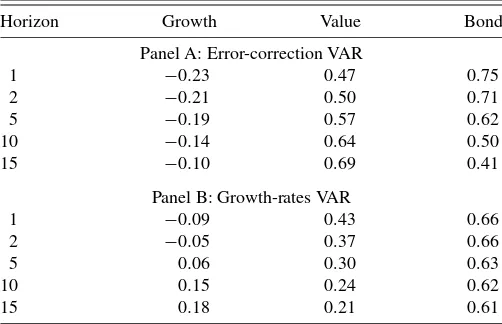
Panel A: Error-correction VAR
1 −0.23 0.47 0.75 2 −0.21 0.50 0.71 5 −0.19 0.57 0.62 10 −0.14 0.64 0.50 15 −0.10 0.69 0.41
Panel B: Growth-rates VAR
1 −0.09 0.43 0.66 2 −0.05 0.37 0.66 5 0.06 0.30 0.63 10 0.15 0.24 0.62 15 0.18 0.21 0.61
NOTE: This table reports the optimal allocation of Bayesian-type investors with different holding periods. Portfolio weights are presented for the EC-VAR specification (Panel A) and the alternative growth rates-based VAR model (Panel B). Panel A is constructed im-posing “tight” prior on the cointegration vector, centered around one.
We maintain risk aversion of 5 and in the cointegration speci-fication we use the “tight” prior centered at 1. First notice that incorporating parameter uncertainty significantly lowers posi-tions in risky assets, which is similar to the findings ofBarberis (2000). In the VAR specification, investors continue to cut down their allocations to value stocks as the horizon increases— starting at 43%, investment in value firms declines to 21% at the 15-year horizon. Similar to the no-parameter uncertainty case, the allocation to growth increases with the horizon due to the cross-sectional diversification effect. With the EC-VAR speci-fication, the allocation to value increases with the investment horizon: from 47% at the one-year horizon to 69% under the 15-year buy-and-hold strategy. Consequently, for both specifi-cations, parameter uncertainty affects the scale of the position, but does not affect the horizon pattern in allocations.
Table7highlights the effect of parameter uncertainty under various assumptions of the prior confidence about the cointe-gration parameter. The optimal portfolio weights are reported for four configurations based on high and low risk aversion,
Table 7. Optimal allocation strategy with parameter uncertainty under various assumptions
Horizon Growth Value Bond Growth Value Bond
RA=5, tight prior RA=5, loose prior
1 −0.23 0.47 0.75 −0.14 0.46 0.68 2 −0.21 0.50 0.71 −0.11 0.47 0.64 5 −0.19 0.57 0.62 −0.05 0.49 0.56 10 −0.14 0.64 0.50 0.04 0.49 0.47 15 −0.10 0.69 0.41 0.11 0.50 0.39
RA=10, tight prior RA=10, loose prior
1 −0.11 0.22 0.88 −0.08 0.23 0.86 2 −0.10 0.25 0.85 −0.07 0.24 0.83 5 −0.09 0.32 0.77 −0.05 0.25 0.79 10 −0.06 0.37 0.69 0.00 0.25 0.75 15 −0.01 0.37 0.64 0.03 0.24 0.73
NOTE: This table reports the optimal allocation of investors who rely on the EC-VAR specification and incorporate parameter uncertainty. Four panels present portfolio weights for different levels of investors’ risk aversion and their confidence that value and growth firms’ dividends exhibit a unit cointegration with aggregate consumption.
and “tight” and “loose” priors about the cointegration parame-ter. As expected, for a given prior, increasing the risk aversion shifts the allocation away from risky assets toward the T-bond. At the same time, both high and low risk aversion investors continue to hold on to value stocks. Although the allocation to growth increases with the horizon, it fails to keep up with the value investment. Further, for a given risk aversion, differ-ent prior beliefs do not dramatically affect portfolio weights at short horizons. The prior uncertainty, however, seems to matter for longer holding periods. With lax beliefs about the cointe-gration parameter, the long-horizon allocation to value stocks scales down relative to a tighter prior.
The key message of the evidence presented above is that the EC-VAR view of return dynamics significantly alters as-set allocations, particularly at long horizons. Specifically, in the long run, value stocks seem to be far more attractive relative to the traditional VAR model for returns. Moreover, this result continues to hold even after accounting for uncertainty about model parameters. In the next section, we discuss the effect of the error-correction channel within the conditional frame-work.
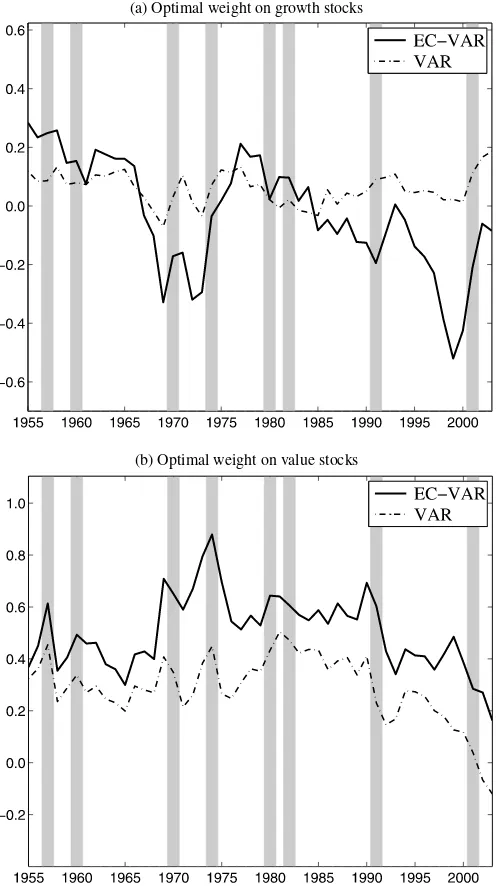
4.2.2 Conditional Analysis. The optimal allocation of a conditional-type investor with the 10-year horizon is presented in Figure 2. We report the evidence for the case where pa-rameter uncertainty about cointegration is incorporated using “loose” prior around unity and risk aversion of 10. The portfo-lio choice problem is solved for each date using the predictive density and the current value of the predictive state variables that are observable to the investor. Portfolio allocation prob-lems that exploit market timing in somewhat different settings are also considered inLynch and Balduzzi(2000),Ferson and Siegel(2001),Brandt and Ait-Sahalia(2001),Ang and Bekaert (2002),Bansal, Dahlquist, and Harvey(2004), andBrandt and Santa-Clara(2006) among others. The importance of condition-ing information and predictability is highlighted in the earlier work ofHansen and Richard(1987).
Figure2suggests a number of interesting observations. The first-order difference between the EC-VAR and the VAR spec-ifications is the difference in level allocations to value and growth firms. Similar to the unconditional analysis, the allo-cation to value is much higher under the EC-VAR specifica-tion. Second, a visual inspection of EC-VAR weights reveals an interesting business-cycle pattern in investment decisions of long-horizon investors. The holding of growth stocks tends to significantly decline at the outset of economic troughs. For ex-ample, the 10-year allocation to growth falls right before the recessions of 1970, 1973, 1990–1991, and 2001. A lag be-tween a decrease in growth weight and an up-coming down-turn measured by the National Bureau for Economic Research (NBER) business cycle indicator is about two to three years. Value holdings, on the other hand, strengthen during recessions. Table 8 summarizes business-cycle properties of conditional allocations by averaging portfolio weights across the NBER-dated expansions and recessions. As the table suggests, the op-timal allocation to value stocks tends to be higher during re-cessions than booms. For example, the mean of the one-year allocation to value is about 50% when the economy is in a low state and only 24% in a high state. This difference, although somewhat less pronounced, is still noticeable at longer
(a) Optimal weight on growth stocks
(b) Optimal weight on value stocks
Figure 2. Portfolio weights. This figure displays time-series of optimal portfolio holdings of growth (a) and value (b) stocks for buy-and-hold investors with the 10-year investment horizons. Thick line corresponds to weights implied by the EC-VAR model, dash-dotted line is derived from the alternative growth rates-based VAR specification. Both allocations incorporate parameter uncertainty and assume risk aversion of 10. The prior of the cointegration parame-ter in the EC-VAR specification is “loose” and cenparame-tered around 1.
zons. Notice also that bond holdings are highly pro-cyclical, increasing during expansions (i.e., when expected returns on equity are low) and declining when the economy moves down (i.e., when risk compensations are expected to rise). The market timing dimension is much less pronounced in the VAR setup. In particular, the correlation between the 10-year allocation to value and consumption growth is−17% in the EC-VAR spec-ification but only −6% in the case of the VAR specification. The corresponding numbers for the five-year horizon are−30% and −15% for the EC-VAR and the standard VAR, respec-tively.
Table 8. Optimal allocations of a Bayesian, conditional-type EC-VAR investor
Horizon Growth Value Bond
Panel A: Average across NBER recessions
1 −0.08 0.50 0.58 5 −0.10 0.54 0.55 10 −0.01 0.60 0.41
Panel B: Average across NBER expansions
1 −0.12 0.24 0.88 5 −0.10 0.39 0.71 10 −0.03 0.48 0.55
NOTE: This table reports optimal allocations of a conditional-type investor who relies on the EC-VAR specification and incorporates parameter uncertainty. Panels A and B report average allocations across economic recessions and expansions as defined by the NBER business cycle indicator over the period from 1954 to 2003. The prior of the cointegration parameter is “loose” and centered around 1, the level of risk aversion is set at 10.
5. CONCLUSION
In this article, we argue that the long-run equilibrium rela-tion measured via a stochastic cointegrarela-tion between aggregate consumption and dividends has significant implications for div-idend growth rates and return dynamics. The error-correction mechanism between dividends and consumption and the ensu-ing EC-VAR provide an alternative specification for describensu-ing the dynamics of equity returns relative to the traditional VAR that ignores the implications of the long-run equilibrium. The recent long-run risks literature (including Bansal and Yaron 2004; Bansal, Dittmar, and Lundblad 2005; Hansen, Heaton, and Li 2005; andBansal, Dittmar, and Kiku 2009) argued that the long-run relation between cash flows and consumption con-tains important information about asset risk premia. Our ap-proach explores the implications of these ideas for optimal port-folio decisions across different investment horizons.
We show that the error-correction channel, incorporated by the EC-VAR representation, significantly alters return fore-casts and the variance–covariance matrix of asset returns and shifts the optimal portfolio mix relative to the traditional VAR. The standard VAR specification captures the short-run return dynamics, but in the presence of cointegration, considerably misses the long-horizon dynamics of asset returns. In contrast, the EC-VAR specification successfully accounts for both short and long-horizon return dynamics. Consequently, as we show, the EC-VAR model is able to capture much larger benefits of time-diversification than the standard VAR framework does.
Incorporating parameter uncertainty in the cointegration-based specification, we highlight the effect of estimation er-rors on long-horizon asset allocations. We show that significant differences in the optimal portfolio decisions between the EC-VAR and EC-VAR specifications persist even after accounting for parameter uncertainty. In sum, our evidence suggests that op-timal allocations derived from the standard VAR may be quite suboptimal for investors with intermediate and long investment horizons.
APPENDIX A: EVALUATING THE ACCURACY OF LOG–LINEARIZATION
To assess the effect of log-linearization (Equation (8)) on the dynamics of multihorizon returns, we perform the following
simulation exercise. Using the point estimates of the EC-VAR specification, we simulate price and dividend levels and con-struct exact asset returns. Innovations are drawn from a normal distribution using the residual variance–covariance matrix. The length of the simulated sample is set at 50 years as in the ac-tual data. Using the simulated sample, we estimate two error-correction specifications: one that directly incorporates the re-turn projection and another one that excludes the rere-turn equa-tion. In the latter case, we use the log-linear approximation to infer the dynamics of asset returns. We iterate on each specifi-cation to compute means and variances of multiperiod returns. Notice that any differences in return moments between the two specifications are driven entirely by the approximation error. Consistent with the evaluation in Campbell and Shiller (1988), we find that differences between exact and approximate returns are tiny at short horizons. However, as the horizon increases, the approximation error is magnified due to compounding and may lead to differences in standard deviations as high as 2% to 4%. For example, at the 15-year horizon, it is quite likely that the volatility of the approximate return on value stocks will over or understate the true return volatility by 3% or 4.2%, respec-tively. For growth stocks, the magnitude of the approximation error can be as large as 2% to 3%. In relative terms, the approx-imation error may lead to up to 15% to 20% distortion in return volatilities at long horizons, which can be significant from an asset allocation perspective. Similar results hold for the VAR specification.
APPENDIX B: INCORPORATING UNCERTAINTY IN THE VAR FRAMEWORK
To obtain the posterior distribution of the VAR parame-ters, we follow Bauwens, Lubrano, and Richard (1999) and re-write the model in the form of seemingly unrelated regres-sions. Specifically, we present the dynamics of each variablei
(i=1, . . . ,n) as
Xi=Ziβi+Ui, (B.1)
whereXiis((T−1)×1)-vector of observations on theith vari-able,Ziis the((T−1)×ki)-matrix of relevant predictors,βi is the (ki×1)-vector of regression coefficients (including the intercept), andUiis the((T−1)×1)-vector of shocks. Stack-ing all the equations together, we can express Equation (B.1) compactly as
x=zβ+u, (B.2)
wherex=(X′1, . . . ,X′n),β=(β1′, . . . ,β′n),u=(U′1, . . . ,U′n), and z=diag(Z1, . . . ,Zn). Alternatively, the EC-VAR model can be cast in the following matrix form:
X=ZB+U, (B.3)
whereX=(X1, . . . ,Xn),Z=(Z1, . . . ,Zn),U=(U1, . . . ,Un), andB=diag(β1, . . . ,βn). To derive the posterior distribution, we assume that investors have no well-defined beliefs about the model parameters, and therefore, use a noninformative prior
ϕ(β,u)∝ |u|−(n+1)/2. (B.4)
As shown inBauwens, Lubrano, and Richard(1999), the pos-terior density of the parameters can be factorizes as
β|u∼Nβˆ,[z′(u−1⊗IT−1)z]−1,
(B.5)
u|β∼IW(Q,T−1), where
ˆ
β= [z′(u−1⊗IT−1)z]−1z′(−u1⊗IT−1)x,
Q=(X−ZB)′(X−ZB).
Although marginal posterior densities of β and u are not available, the posterior analysis can be easily implemented by applying block-Gibbs sampling algorithm to the above condi-tional densities. Specifically, at thejth simulation, we drawβj
conditional on the previousju−1, and close the loop by sam-plingju|βj from the inverse Wishart distribution. The chain is initialized using point estimates of the model parameters. We make two adjustments to the described sampling procedure. We discard the first 500 draws in order to eliminate the influence of the starting values. In addition, to ensure stationarity, we re-move draws if matrixBhas any eigenvalues larger than 0.98.
Our final sample consists of 20,000 draws of parameter values from the posterior, {βj,ju}. We cast them back into the original VAR representation and calculate the means and variance–covariance matrices of multihorizon returns. The cor-responding moments of the predictive distribution of asset re-turns are obtained by taking averages of the constructed quanti-ties. This procedure delivers the term-structure of expected re-turns and risks conditioned only on the observed data, but not the VAR estimates.
APPENDIX C: INCORPORATING UNCERTAINTY IN THE EC–VAR FRAMEWORK
The approach of incorporating uncertainty in the cointegra-tion vector along with the EC-VAR parameters is similar to the one discussed in AppendixB. After observing the sample, in-vestors update their prior to form the posterior distribution of the model parameters. Lettingf0(α)denote the prior density
of the elements of the cointegration vectorα≡(τ0, τ1, δ)′ and
maintaining the noninformative prior for the EC-VAR parame-ters, we can summarize investors’ ex ante beliefs in a composite form,
ϕ(α,β,u)∝f0(α)|u|−(n+1)/2. (C.1) The conditional posterior densities are then given by
β|u,α∼Nβˆ,[z′(−u1⊗IT−1)z]−1,
u|β,α∼IW(Q,T−1), (C.2)
f(α)∝ f0(α)
|α′W0α|l0
|α′W 1α|l1
,
whereβˆ andQare defined as previously and matricesW0,W1
and constantsl0,l1depend on the observed sample (for detailed
formulas seeBauwens and Lubrano 1996). Notice that the an-alytical expression for the conditional density of the cointegra-tion parameter is not available. As suggested inBauwens, Lu-brano, and Richard(1999),f(α), in this case, can be simulated