Climate Change Lines of Evidence

answers to common questions about the science

of climate change

EVIDENCE,

IMPACTS,

AND

CHOICES

CLIMATE

CONTENTS

Part I. Evidence for Human-Caused Climate Change

2

How do we know that Earth has warmed?

3

How do we know that greenhouse gases lead to warming?

4

How do we know that humans are causing greenhouse gases to increase?

6

How much are human activities heating Earth?

9

How do we know the current warming trend isn’t caused by the Sun?

11

How do we know the current warming trend isn’t caused by natural cycles?

12

What other climate changes and impacts have been observed?

15

The Ice Ages

18

Part II. Warming, Climate Changes, and Impacts

in the 21st Century and Beyond

20

How do scientists project future climate change?

21

How will temperatures be affected?

22

How is precipitation expected to change?

23

How will sea ice and snow be affected?

26

How will coastlines be affected?

26

How will ecosystems be affected?

28

How will agriculture and food production be affected?

29

Part III. Making Climate Choices

30

How does science inform emissions choices?

31

What are the choices for reducing greenhouse gas emissions?

32

What are the choices for preparing for the impacts of climate change?

34

Why take action if there are still uncertainties about the risks of climate change?

35

Just what is climate? Climate is commonly thought of as the expected weather conditions

at a given location over time. People know when they go to New York City in winter, they

should take a coat. When they visit the Pacific Northwest, they take an umbrella. Climate

can be measured at many geographic scales—for example, cities, countries, or the

entire globe—by such statistics as average temperatures, average number of rainy days,

and the frequency of droughts. Climate

change

refers to changes in these statistics

over years, decades, or even centuries.

Enormous progress has been made in increasing our understanding of climate change

and its causes, and a clearer picture of current and future impacts is emerging. Research

is also shedding light on actions that might be taken to limit the magnitude of climate

change and adapt to its impacts.

This booklet is intended to help people understand what is known about climate change.

First, it lays out the evidence that human activities, especially the burning of fossil fuels,

are responsible for much of the warming and related changes being observed around

the world. Second, it summarizes projections of future climate changes and impacts

expected in this century and beyond. Finally, the booklet examines how science can help

inform choices about managing and reducing the risks posed by climate change. The

information is based on a number of National Research Council reports (see inside back

cover), each of which represents the consensus of experts who have reviewed hundreds of

studies describing many years of accumulating evidence.

CLIMA

TE CHANGE

But how has this conclusion been reached? Climate science,

like all science, is a process of collective learning that

relies on the careful gathering and analyses of data,

the formulation of hypotheses, the development of

models to study key processes and make testable

predictions, and the combined use of observations

and models to test scientific understanding.

Scientific knowledge builds over time as new

observations and data become available.

Confidence in our understanding grows if multiple

lines of evidence lead to the same conclusions, or

if other explanations can be ruled out. In the case of

climate change, scientists have understood for more

than a century that emissions from the burning of fossil

fuels could lead to increases in the Earth’s average surface

temperature. Decades of research have confirmed and extended this

understanding.

T

he overwhelming

majority of climate

scientists agree that

human activities,

especially the burning

of fossil fuels (coal, oil,

and gas), are responsible

for most of the climate

change currently being

observed.

EVI DE NC E

for Human-Caused

Climate Change

S

cientists have been taking widespread measure-ments of Earth’s surface temperature since around 1880. These data have steadily improved and, today, temperatures are recorded by ther-mometers at many thousands of locations, both on the land and over the oceans. Different research groups, including the NASA Goddard Institute for Space Studies, Britain’s Hadley Centre for Climate Change, the Japan Meteorological Agency, and NOAA’s National Climatic Data Center have used these raw measurements to produce records of long-term global surface temperature change (Figure 1). These groups work carefully to make sure the data aren’t skewed by such things as

changes in the instruments taking the measure-ments or by other factors that affect local tempera-ture, such as additional heat that has come from the gradual growth of cities.

These analyses all show that Earth’s average surface temperature has increased by more than 1.4°F (0.8°C) over the past 100 years, with much of this increase taking place over the past 35 years. A temperature change of 1.4°F may not seem like much if you’re thinking about a daily or seasonal fluctuation, but it is a significant change when you think about a permanent increase averaged across the entire planet. Consider, for example, that 1.4°F is greater than the average annual

FIGURE 2 FIGURE 1

NASA’s Global Surface Temperature Record Esti-mates of global surface temperature change, relative to the average global surface temperature for the period from 1951 to 1980, which is about 14°C (57°F) from NASA Goddard Institute for Space Studies show a warming trend over the 20th century. The esti-mates are based on surface air temperature measure-ments at meteorological stations and on sea surface temperature measurements from ships and satellites. The black curve shows average annual temperatures, and the red curve is a 5-year running average. The green bars indicate the margin of error, which has been reduced over time. Source: National Research Council 2010a

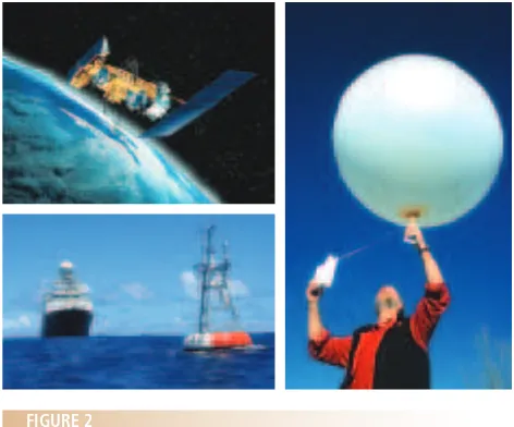
(bottom left) Climate monitoring stations on land and sea, such as the moored buoys of NOAA’s Tropical Atmosphere Ocean (TAO) project, provide real-time data on tempera-ture, humidity, winds, and other atmospheric properties.

Image courtesy of TAO Project Office, NOAA Pacific Marine Environmental Laboratory. (right) Weather balloons, which carry instruments known as radiosondes, provide verti-cal profiles of some of these same properties throughout the lower atmosphere. Image © University Corporation for Atmospheric Research. (top left) The NOAA-N spacecraft, launched in 2005, is the fifteenth in a series of polar-orbiting satellites dating back to 1978. The satellites carry instruments that measure global surface temperature and other climate variables. Image courtesy NASA

E

temperature difference between Washington, D.C., and Charleston, South Carolina, which is more than 450 miles farther south. Consider, too, that a decrease of only 9°F (5°C) in global average temperatures is the estimated difference between today’s climate and an ice age.

In addition to surface temperature, other parts of the climate system are also being monitored carefully (Figure 2). For example, a variety of instruments are used to measure temperature, salinity, and currents beneath the ocean surface. Weather balloons are used to probe the temperature, humidity, and winds in the atmosphere. A key breakthrough in the ability to track global environmental changes began in the 1970s with the dawn of the era of satellite remote sensing. Many different types of sensors, carried on dozens of satellites, have allowed us to build a truly global picture of changes in the temperature

of the atmosphere and of the ocean and land surfaces. Satellite data are also used to study shifts in precipitation and changes in land cover.

Even though satellites measure temperature very differently than instruments on Earth’s surface, and any errors would be of a completely different nature, the two records agree. A number of other indicators of global warming have also been observed (see pp.15-17). For example, heat waves are becoming more frequent, cold snaps are now shorter and milder, snow and ice cover are decreasing in the Northern Hemisphere, glaciers and ice caps around the world are melting, and many plant and animal species are moving to cooler latitudes or higher altitudes because it is too warm to stay where they are. The picture that emerges from all of these data sets is clear and consistent: Earth is warming.

How do we know that greenhouse gases

lead to warming?

A

s early as the 1820s, scientists began to ap-preciate the importance of certain gases in regulating the temperature of the Earth (see Box 1). Greenhouse gases—which include carbon dioxide (CO₂), methane, nitrous oxide, and water vapor— act like a blanket in the atmosphere, keep-ing heat in the lower atmosphere. Although greenhouse gases comprise only a tiny fraction of Earth’s atmosphere, they are critical for keeping the planet warm enough to support life as we know it (Figure 3).

Here’s how the “greenhouse effect” works: as the Sun’s energy hits Earth, some of it is reflected back to space, but most of it is absorbed by the land and oceans. This absorbed

energy is then radiated upward from Earth’s surface in the form of heat. In the absence of greenhouse gases, this heat would simply escape to space, and the planet’s average surface temperature would be well below freezing. But greenhouse

gases absorb and redirect some of this energy downward, keeping

heat near Earth’s surface. As concentrations of

heat-trapping greenhouse gases increase in the

Amplification of the Greenhouse Effect The greenhouse effect is a natural phenomenon that is essential to keeping the Earth’s surface warm. Like a greenhouse window, greenhouse gases allow sunlight to enter and then prevent heat from leaving the atmosphere. These gases include carbon dioxide (CO2), methane (CH4), nitrous oxide (N₂O), and water vapor. Human activities—especially burning fossil fuels—are increasing the concentrations of many of these gases, amplifying the natural greenhouse effect. Image courtesy of the Marian Koshland Science Museum of the National Academy of Sciences

FIGURE 3

E

V

I

DENCE

FOR H

U

MAN-C

AU

SED CLI

MA

TE CHANGE

BOX 1

Early Understanding of Greenhouse Gases

In 1824, French

D

iscerning the human influence on greenhouse gas concentrations is challenging because many greenhouse gases occur naturally in Earth’s atmo-sphere. Carbon dioxide (CO₂)is produced and con-sumed in many natural processes that are part of the carbon cycle (see Figure 4). However, once humans began digging up long-buried forms of carbon such as coal and oil and burning them for energy,

addi-tional CO₂ began to be released into the atmosphere much more rapidly than in the natural carbon cycle. Other human activities, such as cement production and cutting down and burning of forests (deforesta-tion), also add CO₂ to the atmosphere.

Until the 1950s, many scientists thought the oceans would absorb most of the excess CO₂ released by human activities. Then a series of

FIGURE 4

The Carbon Cycle Carbon is continually exchanged between the atmosphere, ocean, biosphere, and land on a variety of timescales. In the short term, CO₂ is exchanged continuously among plants, trees, animals, and the air through respiration and photosynthesis, and between the ocean and the atmosphere through gas exchange. Other parts of the carbon cycle, such as the weathering of rocks and the formation of fossil fuels, are much slower pro-cesses occurring over many centuries. For example, most of the world’s oil reserves were formed when the remains of plants and animals were buried in sediment at the bottom of shallow seas hundreds of millions of years ago, and then exposed to heat and pressure over many millions of years. A small amount of this carbon is released naturally back into the atmosphere each year by volcanoes, completing the long-term carbon cycle. Human activities, espe-cially the digging up and burning of coal, oil, and natural gas for energy, are disrupting the natural carbon cycle by releasing large amounts of “fossil” carbon over a relatively short time period. Source: National Research Council

scientific papers were published that examined the dynamics of carbon dioxide exchange between the ocean and atmosphere, including a paper by oceanographer Roger Revelle and Hans Seuss in 1957 and another by Bert Bolin and Erik Eriksson in 1959. This work led scientists to the hypothesis that the oceans could not absorb all of the CO₂ being emitted. To test this hypothesis, Revelle’s colleague Charles David Keeling began collecting air samples at the Mauna Loa Observatory in Hawaii to track changes in CO₂ concentrations. Today, such measurements are made at many sites around the world. The data reveal a steady increase in atmospheric CO₂ (Figure 5).

To determine how CO₂ concentrations varied prior to such modern measurements, scientists have studied the composition of air bubbles trapped in ice cores extracted from Greenland and Antarctica. These data show that, for at least 2,000 years before

the Industrial Revolution, atmospheric CO₂

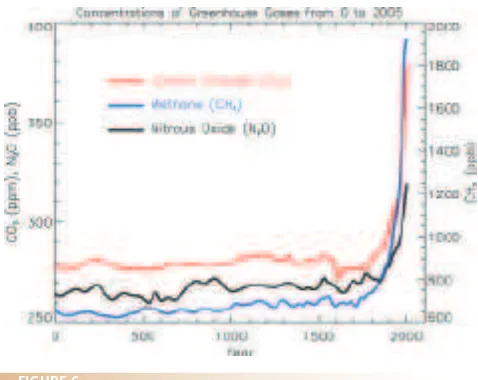
concentrations were steady and then began to rise sharply beginning in the late 1800s (Figure 6). Today, atmospheric CO₂ concentrations exceed 390 parts per million—nearly 40% higher than

preindustrial levels, and, according to ice core data, higher than at any point in the past 800,000 years (see Figure 14, p.18).

Human activities have increased the atmospheric concentrations of other important greenhouse gases as well. Methane, which is produced by the burning of fossil fuels, the raising of livestock, the decay of landfill wastes, the production and transport of natural gas, and other activities, increased sharply through the 1980s before starting to level off at about two-and-a-half times its preindustrial level (Figure 6). Nitrous oxide has increased by roughly 15% since 1750 (Figure 6), mainly as a result of agricultural

E Measurements of Atmospheric Carbon Dioxide

The “Keeling Curve” is a set of careful measurements of atmospheric CO₂ that Charles David Keeling began collecting in 1958. The data show a steady annual increase in CO₂ plus a small up-and-down sawtooth pattern each year that reflects seasonal changes in plant activity (plants take up CO2 during spring and summer in the Northern Hemisphere, where most of the planet’s land mass and land ecosystems reside, and release it in fall and winter).

Source: National Research Council, 2010a

Greenhouse Gas Concentrations for 2,000 Years

fertilizer use, but also from fossil fuel burning and certain industrial processes. Certain industrial chemicals, such as chlorofluorocarbons (CFCs), act as potent greenhouse gases and are long-lived in the atmosphere. Because CFCs do not have natural sources, their increases can be attributed unambiguously to human activities.

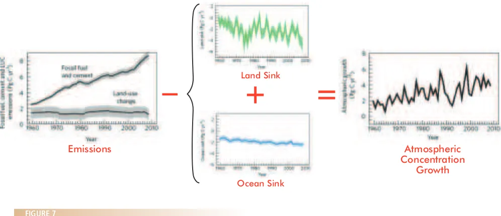
In addition to direct measurements of CO₂ concentrations in the atmosphere, scientists have amassed detailed records of how much coal, oil, and natural gas is burned each year. They also estimate how much CO₂ is being absorbed, on average, by the oceans and the land surface. These

analyses show that about 45% of the CO₂ emitted by human activities remains in the atmosphere. Just as a sink will fill up if water is entering it faster than it can drain, human production of CO₂ is outstripping Earth’s natural ability to remove it from the air. As a result, atmospheric CO₂ levels are increasing (see Figure 7) and will remain elevated for many centuries. Furthermore, a forensic-style analysis of the CO₂ in the atmosphere reveals the chemical “fingerprint” of carbon from fossil fuels (see Box 2). Together, these lines of evidence prove conclusively that the elevated CO₂ concentration in the atmosphere is the result of human activities.

–

+

=

Emissions Atmospheric

Concentration Growth

Land Sink

Ocean Sink

FIGURE 7

Emissions Exceed Nature’s CO₂ Drain Emissions of CO₂ due to fossil fuel burning and cement manufacture are increasing, while the capacity of “sinks” that take up CO2—for example, plants on land and in the ocean—are decreasing. Atmospheric CO₂ is increasing as a result. Source: National Research Council, 2011a

Clues from the “fingerprint” of carbon dioxide.

In a process that takes place over

millions of years, carbon from the decay of plants and animals is stored deep in the Earth’s crust in

the form of coal, oil, and natural gas (see Figure 4). Because this “fossil” carbon is so old, it contains

very little of the radioisotope carbon-14—a form of the carbon that decays naturally over long time

periods. When scientists measure carbon-14 levels in the atmosphere, they find that it is much lower

than the levels in living ecosystems, indicating that there is an abundance of “old” carbon. While a

small fraction of this old carbon can be attributed to volcanic eruptions, the overwhelming majority

comes from the burning of fossil fuels. Average CO

₂

emissions from volcanoes are about 200 million

tons per year, while humans are emitting an estimated 36 billion tons of CO

₂

each year, 80-85% of

which are from fossil fuels.

G

reenhouse gases are referred to as “forcing agents” because of their ability to change the planet’s energy balance. A forcing agent can “push” Earth’s temperature up or down. Greenhouse gases differ in their forcing power. For example, a single methane molecule has about 25 times the warming power of a single CO₂ molecule. However, CO₂ has a much larger overall warming effect than methane because it is much more abundant and stays in the atmosphere for much longer periods of time. Scientists can calculate the forcing power of greenhouse gases based on the changes in their concentrations over time and on physically based calculations of how they transfer energy through the atmosphere.

Some forcing agents push Earth’s energy balance toward cooling, offsetting some of the heating associated with greenhouse gases. For example, some aerosols—which are tiny liquid or solid particles suspended in the atmosphere, such as those that make up most of the visible air pollution—have

a cooling effect because they scatter a portion of incoming sunlight back into

space (see Box 3). Human activities, especially the burning of fossil fuels,

have increased the number of aerosol particles in the atmosphere, especially over and around major urban and industrial areas.

Changes in land use and land cover are another way that human activities are influencing Earth’s climate. Deforestation is responsible for 10% to 20% of the excess CO₂ emitted to the atmosphere each year, and, as has already been discussed, agriculture contributes nitrous oxide and methane. Changes in land use and land cover also modify the reflectivity of Earth’s surface; the more reflective a surface, the more sunlight is sent back into space. Cropland is generally more reflective than an undisturbed forest, while urban areas often reflect less energy than undisturbed land. Globally, human land use changes are estimated to have a slight cooling effect.

When all human and natural forcing agents are considered together, scientists have calculated that the net climate forcing between 1750 and 2005 is

E

How much are human activities

heating Earth?

Warming and Cooling Effects of Aerosols

Aerosols are tiny liquid or solid particles

suspended in the atmosphere that come from a number of human activities, such as fossil fuel

combustion, as well as natural processes, such as dust storms, volcanic eruptions, and sea spray

emissions from the ocean. Most of our visible air pollution is made up of aerosols. Most aerosols

have a cooling effect, because they scatter a portion of incoming sunlight back into space, although

some particles, such as dust and soot, actually absorb some solar energy and thus act as warming

agents. Many aerosols also enhance the reflection of sunlight back to space by making clouds

brighter, which results in additional cooling. Many nations, states, and communities have taken

action to reduce the concentrations of certain air pollutants such as the sulfate aerosols responsible

for acid rain. Unlike most of the greenhouse gases released by human activities, aerosols only

remain in the atmosphere for a short time—typically a few weeks.

pushing Earth toward warming (Figure 8). The extra energy is about 1.6 Watts per square meter of Earth’s surface. When multiplied by the surface area of Earth, this energy represents more than 800 trillion Watts (Terawatts)—on a per year basis, that’s about 50 times the amount of energy people consume from all energy sources combined! This extra energy is being added to Earth’s climate system every second of every day.

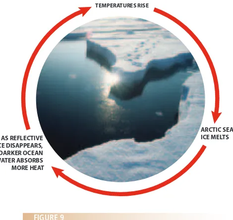
The total amount of warming that will occur in response to a climate forcing is determined by a variety of feedbacks, which either amplify or dampen the initial warming. For example, as Earth warms, polar snow and ice melt, allowing the darker colored land and oceans to absorb more heat—causing Earth to become even warmer, which leads to more snow and ice melt, and so on (see Figure 9). Another impor-tant feedback involves water vapor. The amount of water vapor in the atmosphere increases as the ocean surface and the lower atmosphere warm up; warm-ing of 1°C (1.8°F) increases water vapor by about 7%. Because water vapor is also a greenhouse gas, this increase causes additional warming. Feedbacks that reinforce the initial climate forcing are referred to in the scientific community as positive, or ampli-fying, feedbacks.

There is an inherent time lag in the warming that is caused by a given climate forcing. This lag occurs because it takes time for parts of Earth’s climate systems—especially the massive oceans—to warm or cool. Even if we could hold all human-produced forcing agents at present-day values, Earth would continue to warm well beyond the 1.4°F already ob-served because of human emissions to date.

Warming and Cooling Influences on Earth Since 1750 The warming and cooling influences (measured in Watts per square meter) of various cli-mate forcing agents during the Industrial Age (from about 1750) from human and natural sources has been calculated. Human forcing agents include increases in greenhouse gases and aerosols, and changes in land use. Major volcanic eruptions produce a temporary cooling effect, but the Sun is the only major natural factor with a long-term effect on climate. The net ef-fect of human activities is a strong warming influence of more than 1.6 Watts per square meter. Source: Na-tional Research Council, 2010a (Depiction courtesy U.S. Global Climate Research Program)

Energy (Watts/m2₎

Climate Feedback Loops The amount of warming that occurs because of increased greenhouse gas emissions depends in part on feedback loops. Positive (amplifying) feedback loops increase the net temperature change from a given forcing, while negative (damping) feedbacks offset some of the temperature change associated with a climate forcing. The melting of Arctic sea ice is an example of a positive feedback loop. As the ice melts, less sunlight is reflected back to space and more is absorbed into the dark ocean, causing further warming and further melting of ice. Source: National Research Council, 2011d

A

nother way to test a scientific theory is to in-vestigate alternative explanations. Because the Sun’s output has a strong influence on Earth’s temperature, scientists have examined records of solar activity to determine if changes in solar output might be responsible for the observed global warm-ing trend. The most direct measurements of solar output are satellite readings, which have been avail-able since 1979. These satellite records show that

the Sun’s output has not shown a net increase dur-ing the past 30 years (Figure 10) and thus cannot be responsible for the warming during that period.

Prior to the satellite era, solar energy output had to be estimated by more indirect methods, such as records of the number of sunspots observed each year, which is an indicator of solar activity. These indirect methods suggest there was a slight increase in solar energy reaching Earth during the first few

Measures of the Sun’s Energy

Satellite measurements of the Sun’s energy incident on Earth, available since 1979, show no net increase in solar forcing during the past 30 years. They show only small periodic variations associated with the 11-year solar cycle.

Source: National Research Council, 2010a

Warming Patterns in the Layers of the Atmosphere Data from weather balloons and satellites show a warming trend in the troposphere, the lower layer of the atmosphere, which extends up about 10 miles (lower graph), and a cooling trend in the stratosphere, which is the layer immediately above the troposphere (upper graph). This is exactly the pattern expected from increased greenhouse gases, which trap energy closer to the Earth’s surface.

Source: National Research Council, 2010a

FIGURE 11 FIGURE 10

E

V

I

DENCE

FOR H

U

MAN-C

AU

SED CLI

MA

TE CHANGE

decades of the 20th century. This increase may have contributed to global temperature increases during that period, but does not explain warming in the latter part of the century.

Further evidence that current warming is not a result of solar changes can be found in the temperature trends in the different layers of the atmosphere. These data come from two sources: weather balloons, which have been launched twice daily from hundreds of sites worldwide since the late 1950s, and satellites, which have monitored the temperature of different layers of the

atmosphere since the late 1970s. Both of these data sets have been heavily scrutinized, and both show a warming trend in the lower layer of the atmosphere (the troposphere) and a cooling trend in the upper layer (the stratosphere) (Figure 11). This is exactly the vertical pattern of temperature changes expected from increased greenhouse gases, which trap energy closer to the Earth’s surface. If an increase in solar output were responsible for the recent warming trend, the vertical pattern of warming would be more uniform through the layers of the atmosphere.

How do we know that the current warming

trend is not caused by natural cycles?

D

etecting climate trends is complicated by the fact that there are many natural variations in temperature, precipitation, and other climate variables. These natural variations are caused by many different processes that can occur across a wide range of timescales—from a particularly warm summer or snowy winter to changes over many millions of years.

Among the most well-known short-term cli-matic fluctuations are El Niño and La Niña, which are periods of natural warming and cooling in the tropical Pacific Ocean. Strong El Niño and La Niña events are associated with significant year-to-year changes in temperature and rainfall patterns across many parts of the planet, including the United States. These events have been linked to a number of extreme weather events, such as the 1992 flood-ing in midwestern states and the severe droughts in southeastern states in 2006 and 2007. Globally,

temperatures tend to be higher during El Niño periods, such as

1998, and lower during La Niña years, such as 2008. However, these up-and-down fluctuations are smaller than the 20th cen-tury warming trend; 2008 was still quite a warm year in the long-term record.

strong El Niño and La Niña events, but an overall warming trend is still evident (Figure 12).

In order to put El Niño and La Niña events and other short-term natural fluctuations into perspec-tive, climate scientists examine trends over several decades or longer when assessing the human influ-ence on the climate system. Based on a rigorous as-sessment of available temperature records, climate forcing estimates, and sources of natural climate variability, scientists have concluded that there is a more than 90% chance that most of the observed global warming trend over the past 50 to 60 years can be attributed to emissions from the burning of fossil fuels and other human activities.

Such statements that attribute climate change to human activities also rely on information from

FIGURE 12

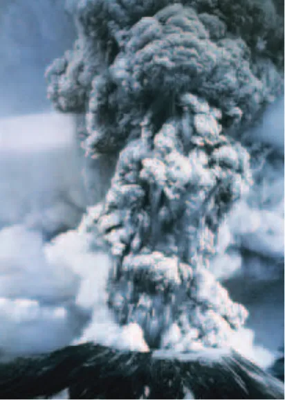
Short-term Temperature Effects of Natural Climate Variations

Natural factors, such as volcanic eruptions and El Niño and La Niña events, can cause average global temperatures to vary from one year to the next, but cannot explain the long-term warming trend over the past 60 years. Image courtesy of the Marian Koshland Science Museum

E

V

I

DENCE

FOR H

U

MAN-C

AU

SED CLI

MA

TE CHANGE

FIGURE 13

climate models (see Box 4). Scientists have used these models to simulate what would have happened if humans had not modified Earth’s climate during the 20th century—that is, how global tempera-tures would have evolved if only natural factors (volcanoes, the Sun, and internal climate variability) were influencing the climate system. These

“undis-turbed Earth” simulations predict that, in the ab-sence of human activities, there would have been negligible warming, or even a slight cooling, over the 20th century. When greenhouse gas emissions and other activities are included in the models, how-ever, the resulting surface temperature changes more closely resemble the observed changes (Figure 13).

What are climate models?

For several decades, scientists have used the world’s most

ad-vanced computers to simulate the Earth’s climate. These models are based on a series of

mathemati-cal equations representing the basic laws of physics—laws that govern the behavior of the

atmo-sphere, the oceans, the land surface, and other parts of the climate system, as well as the interactions

among different parts of the system. Climate models are important tools for understanding past,

present, and future climate change. Climate models are tested against observations so that scientists

can see if the models correctly simulate what actually happened in the recent or distant past.

Image

courtesy Marian Koshland Science Museum

BOX 4

E VA P O R AT I O N C O N D E N S AT I O N &

C O N V E C T I O N

E X C H A N G E O F H E AT & G A S E S B E T W E E N AT M O S P H E R E ,

S E A I C E & O C E A N

G L A C I E R M E LT R A D I AT I V E

E X C H A N G E

T E R R E S T R I A L CA R B O N C Y C L E

O C E A N CA R B O N C Y C L E O C E A N C I R C U L AT I O N WAT E R S T O R A G E

I N I C E & S N O W S U R FA C E R U N - O F F

A I R P O L L U T I O N W I N D

C L O U D S & WAT E R VA P O R

R

ising temperatures due to increasing greenhouse gas concentrations have produced distinct pat-terns of warming on Earth’s surface, with stronger warming over most land areas and in the Arctic. There have also been significant seasonal differences in observed warming. For example, the second half of the 20th century saw intense winter warming across parts of Canada, Alaska, and northern Europe and Asia, while summer warming was particularly strong across the Mediterranean and Middle East and some other places, including parts of the U.S. west (Figure 15). Heat waves and record high tem-peratures have increased across most regions of the world, while cold snaps and record cold tempera-tures have decreased.

Global warming is also having a significant im-pact on snow and ice, especially in response to the strong warming across the Arctic. For example, the average annual extent of Arctic sea ice has dropped by roughly 10% per decade since

satel-lite monitoring began in 1978 (Figure 16). This melting has been especially strong in late summer, leaving large parts of the Arctic Ocean ice-free for weeks at a time and raising questions about effects on ecosystems, commercial shipping routes, oil and gas exploration, and national defense. Many of the world’s glaciers and ice sheets are melting in response to the warming trend, and long-term av-erage winter snowfall and snowpack have declined in many regions as well, such as the Sierra Nevada mountain range in the western United States.

Much of the excess heat caused by human-emit-ted greenhouse gases has warmed the world’s oceans during the past several decades. Water ex-pands when it warms, which leads to sea-level rise. Water from melting glaciers, ice sheets, and ice caps also contributes to rising sea levels. Measurements made with tide gauges and augmented by satellites show that, since 1870, global average sea level has risen by about 8 inches (0.2 meters). It is estimated

E

Patterns of Warming in Winter and Summer Twenty-year average temperatures for 1986-2005 compared to 1955-1974 show a distinct pattern of winter and summer warming. Winter warming has been intense across parts of Canada, Alaska, northern Europe, and Asia, and summers have warmed across the Mediterranean and Middle East and some other places, including parts of the U.S. west. Projections for the 21st century show a similar pattern. Source: National Research Council, 2011a

that roughly one-third of the total sea-level rise over the past four decades can be attributed to ocean expansion, with most of the remainder due to ice melt (Figure 17).

Because CO₂ reacts in seawater to form carbonic acid, the acidification of the world’s oceans is an-other certain outcome of elevated CO₂ concentra-tions in the atmosphere (Figure 18). It is estimated that the oceans have absorbed between one-quarter and one-third of the excess CO₂ from human activi-ties, becoming nearly 30% more acidic than during preindustrial times. Geologically speaking, this large change has happened over a very short timeframe, and mounting evidence indicates it has the poten-tial to radically alter marine ecosystems, as well as the health of coral reefs, shellfish, and fisheries.

Another example of a climate change observed during the past several decades has been changes in

the frequency and distribution of precipitation. Total precipitation in the United States has increased by about 5% over the past 50 years, but this has not been geographically uniform—conditions are gener-ally wetter in the Northeast, drier in the Southeast, and much drier in the Southwest.

Warmer air holds more water vapor, which has led to a measurable increase in the intensity of

precipita-FIGURE 16

Loss of Arctic Sea Ice Satellite-based measurements show a steady decline in the amount of September (end of summer) Arctic sea ice extent from 1979 to 2009 (expressed as a percentage difference from 1979-2000 average sea ice extent, which was 7.0 million square miles). The data show substantial year-to-year variability, but a long-term decline in sea ice of more than 10% per decade is clearly evident, highlighted by the dashed line. Source: National Research Council, 2010a

FIGURE 17

Contributors to Sea-Level Rise

Sea level has risen steadily over the past few decades due to various contributors: thermal expansion in the upper 700 meters of ocean (red) and deeper ocean layers (orange), meltwater from Antarctic and Green-land ice sheets (blue), meltwater from glaciers and ice caps (purple), and water storage on land (green).

tion events. In the United States, for example, the fraction of total precipitation falling in the heaviest 1% of rainstorm increased by about 20% over the past century, with the northeastern states experienc-ing an increase of 54%. This change has increased the risk of flooding and puts additional stress on sewer and stormwater management systems.

As the climate has changed, many species have shifted their range toward the poles and to higher altitudes as they try to stay in areas with the same ambient temperatures. The timing of different seasonal activities is also changing. Several plant species are blooming earlier in Spring, and some birds, mammals, fish, and insects are migrating

earlier, while other species are altering their seasonal breeding patterns. Global analyses show these behaviors occurred an average of 5 days earlier per decade from 1970 to 2000. Such changes can disrupt feeding patterns, pollination, and other vital interactions between species, and they also affect the timing and severity of insects, disease outbreaks, and other disturbances. In the western United States, climate change has increased the population of forest pests such as the pine beetle.

The next section describes how observed climate trends and impacts are predicted to continue if emissions of human-produced greenhouse gases are maintained during the next century and beyond.

E

Evidence of Ocean Acidification With excess CO₂ building up in the atmo-sphere, scientists wanted to know if it was also accumulating in the ocean. Studies that began in the mid-1980s show that the concentration of CO2 in ocean water (in blue, calculated from the partial pressure of CO₂ in seawater) has risen in parallel with the increase in atmospheric CO₂ (in red, part of the Keeling curve). At the same time, the ocean has become more acidic, because the CO₂ reacts with seawater to form carbonic acid. The orange dots are direct measurements of pH in surface seawater (lower pH being more acidic), and the green dots are calculated based on the chemical properties of seawater. Source: National Research Council, 2010d

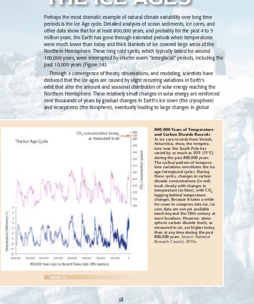
Perhaps the most dramatic example of natural climate variability over long time

periods is the Ice Age cycle. Detailed analyses of ocean sediments, ice cores, and

other data show that for at least 800,000 years, and probably for the past 4 to 5

million years, the Earth has gone through extended periods when temperatures

were much lower than today and thick blankets of ice covered large areas of the

Northern Hemisphere. These long cold spells, which typically lasted for around

100,000 years, were interrupted by shorter warm “interglacial” periods, including the

past 10,000 years (Figure 14).

Through a convergence of theory, observations, and modeling, scientists have

deduced that the ice ages are caused by slight recurring variations in Earth’s

orbit that alter the amount and seasonal distribution of solar energy reaching the

Northern Hemisphere. These relatively small changes in solar energy are reinforced

over thousands of years by gradual changes in Earth’s ice cover (the cryosphere)

and ecosystems (the biosphere), eventually leading to large changes in global

THE ICE AGES

800,000 Years of Temperature and Carbon Dioxide Records

As ice core records from Vostok, Antarctica, show, the tempera-ture near the South Pole has varied by as much as 20°F (11°C) during the past 800,000 years. The cyclical pattern of tempera-ture variations constitutes the ice age/interglacial cycles. During these cycles, changes in carbon dioxide concentrations (in red) track closely with changes in temperature (in blue), with CO2 lagging behind temperature changes. Because it takes a while for snow to compress into ice, ice core data are not yet available much beyond the 18th century at most locations. However, atmo-spheric carbon dioxide levels, as measured in air, are higher today than at any time during the past 800,000 years. Source: National Research Council, 2010a

temperature. The average global

temperature change during an ice age

cycle, which occur over about 100,000

years, is on the order of 9°F ± 2°F (5°C ±

1°C).

The data show that in past ice age

cycles, changes in temperature have

led—that is, started prior to—changes

in CO

₂

. This is because the changes

in temperature induced by changes

in Earth’s orbit around the Sun lead

to gradual changes in the biosphere

and the carbon cycle, and thus CO

₂

,

reinforcing the initial temperature trend.

In contrast, the relatively rapid release of

CO

₂

and other greenhouse gases since

the start of the Industrial Revolution

from the burning of fossil fuel has,

in essence, reversed the pattern: the

additional CO

₂

is acting as a climate

forcing, with temperatures increasing

afterward.

The ice age cycles nicely illustrate

how climate forcing and feedback

effects can alter Earth’s temperature, but

there is also direct evidence from past

climates that large releases of carbon

dioxide have caused global warming.

One of the largest known events of this type is called the Paleocene-Eocene

Thermal Maximum, or PETM, which occurred about 55 million years ago,

when Earth’s climate was much warmer than today. Chemical indicators

point to a huge release of carbon dioxide that warmed Earth by another 9°F

and caused widespread ocean acidification. These climatic changes were

accompanied by massive ecosystem changes, such as the emergence of

many new types of mammals on land and the extinction of many

bottom-dwelling species in the oceans.

The U.S. Geological Survey National Ice Core Lab stores ice cores samples taken from polar ice caps and mountain glaciers. Ice cores provide clues about changes in Earth’s climate and atmosphere going back hundreds of thousands of years.

E

V

I

DENCE

FOR H

U

MAN-C

AU

SED CLI

MA

Fortunately, scientists have made great strides in

predicting the amount of temperature change that

can be expected for different amounts of future

greenhouse gas emissions and in understanding

how increments of globally averaged

temperatures—increases of 1°C, 2°C, 3°C and

so forth—relate to a wide range of impacts.

Many of these projected impacts pose serious

risks to human societies and things people care

about, including water resources, coastlines,

infrastructure, human health, food security, and

land and ocean ecosystems.

Warming, Climate Changes

and

I M PACTS

in the 21st Century and Beyond

Part II

I

n order to respond

T

he biggest factor in determining future global warming is projecting future emissions of CO₂ and other greenhouse gases—which in turn depend on how people will produce and use energy, what national and international policies might be imple-mented to control emissions, and what new tech-nologies might become available. Scientists try to account for these uncertainties by developing differ-ent scenarios of how future emissions—and hence climate forcing—will evolve. Each of these scenarios is based on estimates of how different socioeco-nomic, technological, and policy factors will change over time, including population growth, economic activity, energy-conservation practices, energy tech-nologies, and land use.

Scientists use climate models (see Box 4, p.14) to project how the climate system will respond to different scenarios of future greenhouse gas concen-trations. Typically, many different models are used, each developed by a different modeling team.

Each model uses a slightly different set of mathe-matical equations to represent how the atmosphere, oceans, and other parts of the climate system inter-act with each other and evolve over time. Models are routinely compared with one another and tested against observations to evaluate the accuracy and robustness of model predictions.

The most comprehensive suite of modeling ex-periments to project global climate changes was completed in 2005.1 _{It included 23 different models}

from groups around the world, each of which used the same set of greenhouse gas emissions scenarios. Figure 19 shows projected global temperature changes associated with high, medium-high, and low future emissions (and also the “committed”

FIGURE 19

Projected temperature change for three emissions scenarios Models project global mean temperature change during the 21st century for different scenarios of future emissions—high (red), medium-high (green) and low (blue)— each of which is based on different assumptions of future population growth, economic development, life-style choices, technological change, and avail-ability of energy alternatives. Also shown are the results from “constant concentrations commitment” runs, which assume that atmo-spheric concentrations of greenhouse gases remain constant after the year 2000. Each solid line represents the average of model runs from different modeling using the same scenario, and the shaded areas provide a measure of the spread (one standard devia-tion) between the temperature changes projected by the different models. Source: National Research Council, 2010a

1_{The modeling experiments were part of the World}

Cli-mate Research Programme’s Coupled Model Intercom-parison Project phase 3 (CMIP3) in support of the Inter-governmental Panel on Climate Change (IPPC) Fourth Assessment Report.

warming—warming that will occur as a result of greenhouse gases that have already been emitted). Continued warming is projected for all three future emission scenarios, but sharp differences in global average temperature are clearly evident by the end of the century, with a total temperature increase in

2100, relative to the late 20th century, ranging from less than 2°F (1.1°C) for the low emissions scenario to more than 11°F (6.1°C) for the high emissions scenario. These results show that human decisions can have a very large influence on the magnitude of future climate change.

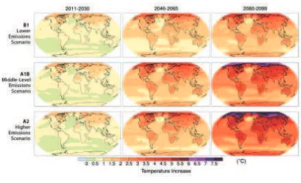
How will temperatures be affected?

L

ocal temperatures vary widely from day to day, week to week, and season to season, but how will they be affected on average? Climate modelers have begun to assess how much of a rise in average temperature might be expected in different regions (Figure 20). The local warmings at each point on the map are first divided by the

correspond-ing amount of global average warmcorrespond-ing and then scaled to show what pattern of warming would be expected. Warming is greatest in the high latitudes of the Northern Hemisphere and is significantly larger over land than over ocean.

As average temperatures continue to rise, the number of days with a heat index above 100°F

FIGURE 20

(the heat index combines temperature and humid-ity to determine how hot it feels) is projected to increase throughout this century (Figure 21). By the end of the century, the center of the United States is expected to experience 60 to 90 ad-ditional days per year in which the heat index is more than 100°F. Heat waves also are expected to last longer as the average global temperature increases. It follows that as global temperatures rise, the risk of heat-related illness and deaths also should rise. Similarly, there is considerable con-fidence that cold extremes will decrease, as will cold-related deaths. The ratio of record high tem-peratures to record low temtem-peratures, currently 2 to 1, is projected to increase to 20 to 1 by mid-century and 50 to 1 by the end of the mid-century for

a mid-range emissions scenario. FIGURE 21

Projections of Hotter Days Model projections sug-gest that, relative to the 1960s and 1970s, the number of days with a heat index above 100°F will increase markedly across the United States. Image courtesy U.S. Global Climate Research Program

How is precipitation expected to change?

G

lobal warming is ex-pected to intensify regional contrasts in precipi-tation that already exist: dry areas are expected to get even drier, and wet areas even wetter. This is because warmer temperatures tend to increase evaporation from oceans, lakes, plants, and

soil, which, according to both theory and observa-tions, will boost the amount of water vapor in the atmosphere by about 7% per 1°C (1.8°F) of warm-ing. Although enhanced evaporation provides more atmospheric moisture for rain and snow in some downwind areas, it also dries out the land surface, which exacerbates the impacts of drought in some regions.

Canada. Most models suggest increased drying in the southwestern United States.

Observations in many parts of the world show a statistically significant increase in the intensity of heavy rainstorms. Computer models indicate that this trend will continue as Earth warms, even in subtropical regions where overall precipitation will decrease. In those regions, the projections show an increase in dry days between rainstorms with the av-erage rainfall over seasons going down. In general, extreme rainstorms are likely to intensify by 5-10% for each 1°C (1.8°F) of global warming, with the greatest intensi-fication in the tropics, where rain is heaviest.

Changes in precipitation will affect annual streamflow, which is roughly equal to the amount of runoff—the water from snow or rain that flows into rivers and creeks. Global climate models indicate that future runoff is likely to decrease

throughout most of the United States, except for parts of the Northwest and Northeast, with particu-larly sharp drops in the Southwest. A decrease in runoff of 5-10% per degree of warming is expected in some river basins, including the Arkansas and the Rio Grande (Figure 23). This decrease would be due mainly to increased evaporation because of higher temperatures, which will not be offset by changes in precipitation. Globally, streamflow in many tem-perate river basins outside Eurasia is likely to de-crease, especially in arid and semiarid regions.

Rising temperatures and increased evaporation and drought can also be

expected to boost the risk of fire in some regions. In general, for-ests that are already fire-prone,

such as the evergreen forests of the western United States and Canada, are likely to become even more vulnerable to fire as temperatures rise. The average area burned by wildfire per year in parts of the western United States is

Precipitation Patterns per Degree Warming Higher temperatures increase evaporation from oceans, lakes, plants, and soil, putting more water vapor in the atmosphere and, in turn, producing more rain and snow in some areas. However, increased evaporation also dries out the land surface, which reduces precipitation in some regions. This figure shows the projected percentage change per 1°C (1.8°F) of global warming for winter (December–Febru-ary, left) and summer (June–August, right). Blue areas show where more precipitation is predicted, and red areas show where less precipitation is predicted. White areas show regions where changes are uncertain at present, be-cause there is not enough agreement among the models used on whether there will be more or less precipitation in those regions. Source: National Research Council, 2011b

expected to increase annually by two to four times per degree of warming (Figure 24). At the same time, areas dominated by shrubs and grasses, such as parts of the Southwest, may experience a reduction in fire over time as warmer temperatures cause shrubs and grasses to die out. In this case, the potential societal benefits of fewer fires would be countered by the loss of existing ecosystems.

FIGURE 24

Increased Risk of Fire Rising temperatures and in-creased evaporation are expected to increase the risk of fire in many regions of the West. This figure shows the percent increase in burned areas in the West for a 1°C increase in global average temperatures relative to the median area burned during 1950-2003. For example, fire damage in the northern Rocky Mountain forests, marked by region B, is expected to more than double annually for each 1°C (1.8°F) increase in global average temperatures. Source: National Research Council, 2011a

W

AR

M

I

NG, CLI

MA

TE CHANGES, AN

D

IMP

A

C

T

S

I

N TH

E 2

1

S

T

CENTU

RY AN

D B

E

Y

ON

D

% change in runoff per degree warming (relative to 1971-2001)

FIGURE 23

A

s global warming continues, the planet’s many forms of ice are decreasing in extent, thickness, and duration. Models indicate that seasonally ice-free condi-tions in the Arctic Ocean are likely to occur before the end of this century and suggest about a 25% loss in Septem-ber sea-ice extent for each 1°C (1.8°F) in global warming.

In contrast to the Arctic, sea ice surrounding Antarctica has, on average, expanded during the past

several decades. This increase may be linked to the stratospheric “ozone hole” over the Antarc-tic, which developed because of the use of ozone-depleting chemicals in refrigerants and spray cans. The ozone hole allows more damaging UV light to get to the lower atmosphere and, in the Antarctic, may have also resulted in lower temperatures as more heat escapes to space. However, this effect is expected to wane as ozone returns to normal levels by later this century, due in part to the success of the Montreal Protocol, an international treaty that

banned the use of ozone-depleting chemicals. Still, Antarctic sea ice may decrease less rapidly than

Arctic ice, in part because the Southern Ocean stores heat

at greater depths than the Arctic Ocean, where the heat can’t melt ice as easily.

In many areas of the globe, snow cover is expect-ed to diminish, with snowpack building later in the cold season and melting earlier in the spring. According to one sensitivity analysis, each 1°C (1.8°F) of local warming may lead to an average 20% reduction in local snowpack in the western United States. Snowpack has impor-tant implications for drinking water supply and hydropower production. In places such as Siberia, parts of Greenland, and Antarctica, where tem-peratures are low enough to support snow over long periods, the amount of snowfall may increase even as the season shortens, because the increased amount of water vapor associated with warmer temperatures may enhance snowfall.

How will sea ice and snow be affected?

How will coastlines be affected?

S

ome of Earth’s most densely populated regions lie at low elevation, making rising sea level a cause for concern. Sea-level rise is projected to continue for centuries in response to human-caused increases in greenhouse gases, with an estimated 0.5-1.0 meter (20-39 inches) of mean sea-level rise by 2100. However, there is evidence that sea-level rise could be greater than expected due to melting of sea ice. Recent studies have shown more rapid than expected melting from glaciers and ice sheets. Observed sea-level rise has been near the top of the range of projections that were made in 1990 (Figure 25).

Quantifying the future threat posed to particular coastlines by rising seas and floods is challeng-ing. Many nonclimatic factors are involved, such as where people choose to build homes, and the risks will vary greatly from one location to the next. Moreover, infrastructure damage is often triggered by extreme events, for example hurricanes and earthquakes, rather than gradual change. However, there are some clear “hot spots,” particularly in large urban areas on coastal deltas, including those of the Mississippi, Nile, Ganges, and Mekong rivers.

affect 5 million to 200 million people worldwide. Up to 4 million people could be permanently displaced, and erosion could claim more than 250,000 square kilometers of wetland and dryland (98,000 square miles, an area the size of Oregon). Relocations are already occurring in towns along the coast of Alaska,

where reductions in sea ice and melting permafrost allow waves to batter and erode the shoreline. Coastal erosion effects at 1.0 meter of sea-level rise would be much greater, threatening many parts of the U.S. coastline (Figure 26).

W

Comparison of Projected and Observed Sea-Level Rise Observed sea-level change since 1990 has been near the top of the range projected by the Intergov-ernmental Panel on Climate Change Third Assessment Report, published in 1990 (gray-shaded area). The red line shows data derived from tide gauges from 1970 to 2003. The blue line shows satellite observations of sea-level change. Source: National Research Council, 2011a

FIGURE 26

Projected Effects of Sea-Level Rise on the U.S. East and Gulf Coasts If sea level were to rise as much as 1 meter (3.3-feet), the areas in pink would be susceptible to coastal flooding. With a 6-me-ter (19.8-foot) rise in sea level, areas shown in red would also be susceptible. The pie charts show the percentage area of some cities that are potentially susceptible at 1-meter and 6-meter sea-level rise.

W

hether marine or terrestrial, all organisms attempt to acclimate to a changing environ-ment or else move to a more favorable location— but climate change threatens to push some species beyond their ability to adapt or move. Special stress is being placed on cold-adapted species on mountain tops and at high latitudes. Shifts in the timing of the seasons and life-cycle events such as blooming, breeding, and hatching are causing mis-matches between species that disrupt patterns of feeding, pollination, and other key aspects of food webs. The ability of species to move and adapt also are hampered by human infrastructural barriers (e.g., roads), land use, and competition or interac-tion with other species.

In the ocean, circulation changes will be a key driver of ecosystem impacts. Satellite data show that warm surface waters are mixing less with cooler, deeper waters, separating near-surface marine life from the nutrients below and ultimately reducing the amount of phytoplankton, which forms the base of the ocean food web (Figure 27). Climate change will exacerbate this problem in the tropics and subtropics. However, in temperate and polar waters, vertical mixing of waters could increase, especially with expected losses in sea ice. At the same time, ocean warming will continue to push the ranges of many marine species toward the poles.

Changing ocean chemistry can result in other impacts—warmer waters could lead to a decline in subsurface oxygen, boosting the risk of “dead zones,” where species high on the food chain are largely absent because of a lack of oxygen. Ocean acidification, brought on as the oceans take in more of the excess CO₂ will threaten many species over time, especially mollusks and coral reefs. But not all life forms will suffer: some types of phytoplankton and other photosynthetic organisms may benefit from increases in CO₂. Ocean acidification will continue to worsen if CO₂ emissions continue un-abated in the decades ahead.

How will ecosystems be affected?

FIGURE 27

Effects on the Ocean Food Web The growth rate of marine phytoplankton, which form the base of the ocean food web, is likely to be reduced over time because of higher ocean surface temperatures. This creates a greater distance between warmer surface waters and cooler deep waters, separating upper ma-rine life from nutrients found in deep water. The figure shows changes in phytoplankton growth (vertically integrated annual mean primary production, or PP), expressed as the percentage difference between 2090-2099 and 1860-1869) per 1°C (1.8°F) of global warm-ing. Source: National Research Council, 2011a

T

he stress of climate change on farming may threaten global food security. Although an increase in the amount of CO₂ in the atmosphere favors the growth of many plants, it does not necessarily translate into more food. Crops tend to grow more quickly in higher temperatures, leading to shorter growing periods

and less time to produce grains. In addition, a changing climate will bring other hazards, including greater water stress and the risk of higher temperature peaks that can quickly damage crops.

Agricultural impacts will vary across regions and by crop. Moderate warming and associated increases in CO₂ and changes in precipitation are expected to benefit crop and pasture lands in middle to high latitudes but decrease yield in seasonally dry and low-latitude areas. In California, where half the nation’s fruit and vegetable crops are grown, climate change is projected to decrease yields of almonds, walnuts, avocados, and table grapes by up to 40 percent by 2050. Regional assessments for other parts of the world consistently conclude that climate change presents serious risk to critical staple crops in sub-Saharan African and in places that rely on

water resources from glacial melt and snowpack.

Modeling indicates that the CO₂-related benefits for some crops will largely be outweighed by negative factors if global tem-perature rises more than 1.0°C (1.8°F) from late 20th-century values (Figure 28), with the following project-ed impacts:

• For each degree of warming, yields of corn in

the United States and Africa, and wheat in India, drop by 5-15%

• Crop pests, weeds, and disease shift in

geographic range and frequency

• If 5°C (9°F ) of global warming were to be

reached, most regions of the world would experience yield losses, and global grain prices would potentially double

Growers in prosperous areas may be able to adapt to these threats, for example by varying the crops which they grow and the times at which they are grown. However, adaptation may be less effective where local warming exceeds 2°C (3.6°F) and will be limited in the tropics, where the growing season is restricted by moisture rather than temperature.

W

Loss of Crop Yields per Degree Warming Yields of corn in the United States and Africa, and wheat in India, are projected to drop by 5-15% per de-gree of global warming. This figure also shows projected changes in yield per degree of warming for U.S. soybeans and Asian rice. The expected impacts on crop yield are from both warming and CO₂ increases, assuming no crop adap-tation. Shaded regions show the likely ranges (67%) of projections. Values of global temperature change are relative to the preindustrial value; current global temperatures are roughly 0.7°C (1.3°F) above that value. Source: National Re-search Council, 2011a

FIGURE 28

As a result, decision makers of all types—including

individuals, businesses, and governments at all levels—

are taking or planning actions to respond to climate

change. Depending on how much emissions are

curtailed, the future could bring a relatively mild

change in climate or it could deliver extreme

changes that could last thousands of years. The

nation’s scientific enterprise can contribute both by

continuing to improve understanding of the causes

and consequences of climate change and by improving

and expanding the options available to limit the magnitude of

climate change and to adapt to its impacts.

Making

Climate

C HOIC ES

Part III

A

s discussed in Part II of this booklet, improve-ments in the ability to predict climate change impacts per degree of warming has made it easier to evaluate the risks of climate change. Policymak-ers are left to address two fundamental questions: (1) at what level of warming are risks acceptable given the cost of limiting them; and (2) what level of emissions will keep Earth within that level of warming? Science cannot answer the first question, because it involves many value judgments outside the realm of science. However, much progress has been made in answering the second.

Even with expected improvements in energy ef-ficiency, if the world continues with “business as usual” in the way it uses and produce energy, CO₂ emissions will continue to accumulate in the atmo-sphere and warm Earth.2 _{As illustrated in Figure 29,}

to keep atmospheric concentrations of CO₂ roughly steady for a few decades at any given level to avoid increasing climate change impacts, global emissions would have to be reduced by 80%.

Another helpful concept is that the amount of warming expected to occur from CO₂ emissions depends on the cumulative amount of carbon emis-sions, not on how quickly or slowly the carbon is added to the atmosphere (Figure 30). Humans have emitted about 500 billion tons (gigatonnes) of car-bon to date. Best estimates indicate that adding about 1,150 billion tons of carbon to the air would lead to a global mean warming of 2°C (3.6°F).

How does science inform

emissions choices?

FIGURE 29

FIGURE 30 Illustrative Example: How Emissions Relate to CO2

Concentrations. Sharp reductions in emissions are needed to stop the rise in atmospheric concentrations of CO₂ and meet any chosen stabilization target. The graphs show how changes in carbon emissions (top panel) are related to changes in atmospheric concen-trations (bottom panel). It would take an 80% reduc-tion in emissions (green line, top panel) to stabilize atmospheric concentrations (green line, bottom panel) for any chosen stabilization target. Stabilizing emis-sions (blue line, top panel) would result in a continued rise in atmospheric concentrations (blue line, bottom panel), but not as steep as a rise if emissions continue to increase (red lines). Source: National Research Council,

2_{Other greenhouse gases are a factor, but CO}

2 is by far

the most important greenhouse gas in terms of long-term climate change effects.