El e c t ro n ic
Jo ur
n a l o
f P
r o
b a b il i t y
Vol. 15 (2010), Paper no. 73, pages 2220–2260. Journal URL
http://www.math.washington.edu/~ejpecp/
Multitype Contact Process on
Z
: Extinction and Interface
Daniel Valesin
1Abstract
We consider a two-type contact process onZin which both types have equal finite range and supercritical infection rate. We show that a given type becomes extinct with probability 1 if and only if, in the initial configuration, it is confined to a finite interval[−L,L]and the other type occupies infinitely many sites both in(−∞,L)and(L,∞). Additionally, we show that if both types are present in finite number in the initial configuration, then there is a positive probability that they are both present for all times. Finally, it is shown that, starting from the configuration in which all sites in(−∞, 0]are occupied by type 1 particles and all sites in(0,∞)are occupied by type 2 particles, the processρt defined by the size of the interface area between the two types at timetis tight.
Key words:Interacting Particle Systems, Interfaces, Multitype Contact Process. AMS 2000 Subject Classification:Primary 60K35.
Submitted to EJP on May 11, 2010, final version accepted November 30, 2010.
1Institut de Mathématiques, Station 8, École Polytechnique Fédérale de Lausanne, CH-1015
Lausanne, Switzerland, [email protected], http://ima.epfl.ch/prst/daniel/index.html
1
Introduction
The contact process onZis the spin system with generator
Ωf(ζ) =X
x
(f(ζx)−f(ζ))c(x,ζ); ζ∈ {0, 1}Z
where
¨
ζx(y) =ζ(y)if x 6= y;
ζx(x) =1−ζ(x); c(x,ζ) =
¨
1 ifζ(x) =1;
λPyζ(y)·p(y−x) ifζ(x) =0;
forλ >0 and p(·) a probability kernel. We take p to be symmetric and to have finite rangeR =
max{x :p(x)>0}.
The contact process is usually taken as a model for the spread of an infection; configuration ζ ∈ {0, 1}Z is the state in which an infection is present at x ∈Zif and only if ζ(x) =1. With this in mind, the dynamics may be interpreted as follows: each infected site waits an exponential time of parameter 1, after which it heals, and additionally each infected site waits an exponential time of parameterλ, after which it chooses, according to the kernelp, some other site to which the infection is transmitted if not already present.
We refer the reader to[13]for a complete account of the contact process. Here we mention only the most fundamental fact. Let ¯ζand0be the configurations identically equal to 1 and 0, respectively,
S(t)the semi-group associated toΩ,Pλ the probability measure under which the process has rateλ
andζ0
t the configuration at timet, started from the configuration where only the origin is infected.
There existsλc, depending onp, such that
• ifλ≤λc, thenPλ(ζ0t 6=0∀t) =0 andδζ¯S(t)→δ0;
• ifλ > λc, thenPλ(ζ0t 6=0∀t)>0 andδζ¯S(t)converges, ast → ∞, to some non-trivial invariant
measure.
Again, see[13]for the proof. Throughout this paper, we fixλ > λc.
The multitype contact process was introduced in[15]as a modification of the above system. Here we consider a two-type contact process, defined as the particle system (ξt)t≥0 with state space
{0, 1, 2}Zand generator
Λf(ξ) = X
x:ξ(x)6=0
(f(ξx,0)−f(ξ))+
X
x:ξ(x)=0
(f(ξx,1)−f(ξ))c1(x,ξ) + (f(ξx,2)−f(ξ))c2(x,ξ)
; ξ∈ {0, 1, 2}Z,
where
¨
ξx,i(y) =ξ(y)if x 6= y;
ξx,i(x) =i,
i=0, 1, 2;
ci(x,ξ) =λPy1{ξ(y)=i}·p(y−x),
i=1, 2.
(1denotes indicator function).
empty regions become occupied at a rate that depends on the number of individuals of each species living in neighboring sites, and this means a new birth. The important point is that occupancy is strong in the sense that, if a site has an individual of, say, type 1, the only way it will later contain an individual of type 2 is if the current individual dies and a new birth occurs originated from a type 2 individual.
Let us point out some properties of the above dynamics. First, it is symmetric for the two species: both die and give birth following the same rules and restrictions. Second, if only one of the two species is present in the initial configuration, then the process evolves exactly like in the one-type contact process. Third, if we only distinguish occupied sites from non-occupied ones, thus ignoring which of the two types is present at each site, again we see the evolution of the one-type contact pro-cess. We also point out that both the contact and the multitype contact processes can be constructed with families of Poisson processes which are interpreted astransmissionsandhealings. These fam-ilies are called graphical constructions, or Harris constructions. Although we will provide formal definitions in the next section, we will implicitly adopt the terminology of Harris constructions in the rest of this Introduction.
The first question we address is: for which initial configurations does a given type (say, type 1) become extinct with probability one? By extinction we mean: for some time t0 (and hence all
t≥t0),ξt0(x)6=1 for allx. We prove
Theorem 1.1. Assume at least one site is occupied by a1inξ0. The1’s become extinct with probability one if and only if there exists L>0such that
(A) ξ0(x)6=1∀x∈/[−L,L]and
(B) #{x ∈(−∞,−L]:ξ0(x) =2}=#{x ∈[L,∞):ξ0(x) =2}=∞.
(# denotes cardinality). This result is a generalization of Theorem 1.1. in[1], which is the exact same statement in the nearest neighbour context (i.e., p(1) = p(−1) =1/2). Although there are some points in common between our proof and the one in that work, our general approach is completely different. Additionally, their methods do not readily apply in our setting, as we now briefly explain. LetL ={ξ∈ {0, 1, 2}Z :ξ(x) = 1,ξ(y) =2=⇒ x < y}. When the range R=1,
ξ0 ∈ L implies ξt ∈ L for all t ≥ 0. In [1], the proof of both directions of the equivalence of
Theorem 1.1 rely on this fact (see for example Corollary 3.1 in that paper), which does not hold for
R>1.
If both types are present in finite number in the initial configuration, there is obviously positive prob-ability that one of them is present for all times, because the process is supercritical. The following theorem says that there is positive probability that they arebothpresent for all times.
Theorem 1.2. Assume that
0<#{x :ξ0(x) =1}, #{x :ξ0(x) =2}<∞.
Then, with positive probability, for all t≥0there exist x,y ∈Zsuch thatξt(x) =1, ξt(y) =2.
Now assume thatR>1. Define the “heaviside” configuration asξh=
1(−∞,0]+2·1(0,∞)and denote
byξt the two-type contact process with initial conditionξ0=ξh. Define
We haveρ0=−1, and at a given timetboth events{ρt>0}and{ρt<0}have positive probability.
Ifρt>0, we call the interval[lt,rt]theinterface area. The question we want to ask is: iftis large,
is it reasonable to expect a large interface? We answer this question negatively.
Theorem 1.3. The law of(ρt)t≥0is tight; that is, for anyε >0, there exists L>0such thatP(|ρt|>
L)< εfor every t≥0.
There are several works concerning interface tightness in one-dimensional particle systems, the first of which is [5], where interface tightness is established for the voter model. Others are[3], [4],
[17]and[2].
In [2], it is shown that interface tightness also occurs on another variant of the contact process, namely the grass-bushes-trees model considered in [8], with both species having same infection rate and non-nearest neighbor interaction. The difference between the grass-bushes- trees model and the multitype contact process considered here is that, in the former, one of the two species, say the 1’s, is privileged in the sense that it is allowed to invade sites occupied by the 2’s. For this reason, from the point of view of the 1’s, the presence of the 2’s is irrelevant. It is thus possible to restrict attention to the evolution of the 1’s, and it is shown that they form barriers that prevent entrance from outside; with this at hand, interface tightness is guaranteed regardless of the evolution of the 2’s. Here, however, we do not have this advantage, since we cannot study the evolution of any of the species while ignoring the other.
Our results depend on a careful examination of the temporal dual process; that is, rather than moving forward in time and following the descendancy of individuals, we move backwards in time and trace ancestries. The dual of the multitype contact process was first studied by Neuhauser in
[15] and may be briefly described as follows. Each site x ∈Z at (primal) time s has a random (and possibly empty)ancestor sequence, which is a list of sites y ∈Zsuch that the presence of an infection in(y, 0)would imply the presence of an infection in(x,s)(in other words, such that there is an infection path connecting(y, 0)and(x,s)). The ancestors on the list are ranked in decreasing order; the idea is that if the first ancestor is not occupied inξ0, then we look at the second, and
so on, until we find the first on the list that is occupied in ξ0, and take its type as the one passed
to x. We denote this sequence(η1,xs,η2,xs, . . .). By moving in time in the opposite direction as that of the original process and using the graphical representation of the contact process for “negative” primal times, we can define theancestry process of x,((η1,xt,η2,xt, . . .))t≥0. The process given by the first element of the sequence,(η1,xt)t≥0, is called thefirst ancestor process. We point out three key properties of the ancestry process:
• First ancestor processes have embedded random walks. In [15]it is proven that, on the event that a site x has a nonempty ancestry at all times t ≥ 0, we can define an increasing sequence of randomrenewal times(τnx)n≥0 with the property that the space-time increments
(η1,xτx n+1−η
x
1,τx n,τ
x n+1−τ
x
n)are independent and identically distributed. This fact enormously
simplifies the study of the first ancestor process, which is not markovian and at first seems very complicated.
which time they coalesce. We give a new approach to formalizing this notion, one that we believe provides a clear understanding of the picture and allows for detailed results.
In order to follow two first ancestor processes simultaneously, we define joint renewals (τnx,y)n≥0 and argue that the law of the processes after a joint renewal only depends on their
initial difference at the instant of the renewal. Thus, the discrete-time process defined by the difference between the two processes at the instants of renewals is a Markov chain onZ. For this chain, zero is an absorbing state and corresponds to coalescence of first ancestors. We also show that, far from the origin, the transition probabilities of the chain become close to a symmetric measure onZ, and from this fact we are able to show that the tail of the distri-bution of the hitting time of 0 for the chain looks like the one associated to a simple random walk onZ. From this construction and estimate we also bound the expected distance between ancestors at a given time.
• Ancestries become sparse with time. Consider the system of coalescing random walks in which each site ofZstarts with one particle at time 0. The density of occupied sites at timet, which is equal to the probability of the origin being occupied, tends to 0 ast → ∞. We prove a similar result for our ancestry sequences. Fix atruncation level N and, at dual time t, mark theN first ancestors of each site at dual time 0 (this gives the set{ηxn,t : 1≤ n≤ N,x ∈Z: the ancestry of x reaches timet}). We show that the density of this random set tends to 0 as
t→ ∞, and estimate the speed of this convergence depending onN.
From this last fact, we can immediately prove Theorem 1.1 under the stronger hypothesis that all sites outside[−L,L]are occupied by 2’s inξ0. To obtain the general case, we then use a structure
called adescendancy barrier, whose existence was established in[2]. Theorem 1.2 is obtained quite easily from Theorem 1.1. The proof of Theorem 1.3 is more intricate, and follows the main steps of
[5], which studies the voter model.
We believe that our results and general approach may prove useful in other questions concerning the multitype contact process, in particular those that relate to almost sure properties of the trajectories
t7→ξt of the process, as opposed to properties of its limit measures.
2
Ancestry process
We will start describing the familiar construction of the one-type contact process from its graphical representation. We will then show how the same representation can be used to construct the mul-titype contact process, present the definition of the ancestry process together with some facts from
[15], and finally prove a simple lemma.
Suppose given a collection of independent Poisson processes on[0,∞):
(Dx)x∈Zwith rate 1, (N(x,y))x,y∈Zwith rateλ·p(y−x).
AHarris construction H is a realization of all such processes. H can thus be understood as a point measure on(Z∪Z2)
×[0,∞). Sometimes we abuse notation and denote the collection of processes itself byH. Given(x,t)∈Z×[0,∞), letθ(x,t)(H)be the Harris construction obtained by shifting
H so that(x,t)becomes the space-time origin. By translation invariance of the space-time construc-tion,θ(x,t)(H)andH have the same distribution. We will also writeH[0,t]to denote the restriction
Given a Harris constructionH and(x,s),(y,t)∈Z×[0,∞)withs< t, we write(x,s)↔(y,t)(in
H) if there exists a piecewise constant, right-continuous functionγ:[s,t]→Zsuch that
•γ(s) =x,γ(t) = y;
•γ(r)6=γ(r−)if and only if r∈N(γ(r−),γ(r));
•∄s≤r≤t withr∈Dγ(r).
One such functionγis called apathdetermined byH. The points in the processes{Dx}are usually calleddeath marks, and the points in{N(x,y)}are calledarrows. Thus, a path can be thought of as a line going up from(x,s)to(y,t)following the arrows and not crossing any death marks.
GivenA⊂Z,(x,t)∈Z×[0,∞)and a Harris constructionH, put
[ζAt(x)](H) =1{For somey∈A,(y,0)↔(x,t)inH}.
Under the law ofH,(ζAt)has the distribution of the contact process with parameterλ, kernelpand initial state1A; see[6]for details. From now on, we omit dependency on the Harris construction
and write (for instance)ζt instead ofζt(H).
Before going into the multitype contact process, we list some properties of the one-type contact process that will be very useful. Fix(x,s) ∈Z×[0,∞) and t >s. Define the time of death and maximal distance traveled until time tfor an infection that starts at(x,s),
T(x,s)=inf{s′>s:∄y:(x,s)↔(y,s′)},
Mt(x,s)=sup{|y−x|:(x,s)↔(y,s′)for somes′∈[s,t]}
(these only depend onH and are thus well-defined regardless ofξs(x)). Whens=0, we omit it and
write Tx,Mtx. IfA⊂Z, we also defineTA=inf{t ≥0 :∄ x ∈A,y ∈Z:(x, 0)↔(y,t)}. We start by observing thatMt(x,s)is stochastically dominated by a multiple of a Poisson random variable, so there existκ,c,C >0 such that
P(Mtx > κt)≤C e−c t ∀x∈Z,t≥0. (2.1)
Remark 2.1. Throughout this paper, letters that denote universal constants whose particular values are irrelevant, such as c,C,κin the above, will have different values in different contexts and will sometimes change from line to line in equations.
Next, since we are takingλ > λc, we haveP(Tx =∞) =P(T0=∞)>0 for allx, and
P(Tx=Ty =∞)≥P(T0=∞)2>0, ∀x,y ∈Z. (2.2)
This follows from the self-duality of the contact process and the fact that its upper invariant measure has positive correlations; see[12]. Our last property is that there existc,C >0 such that, for any
A⊂Zandt>0,
P(t <TA<∞)≤C e−c t. (2.3)
For the case R = 1, this is Theorem 2.30 in [13]. The proof uses a comparison with oriented percolation and can be easily adapted to the caseR>1.
We now turn to our treatment of the multitype contact process and its dual, the ancestry process, through graphical constructions. We will proceed in three steps.
already occupied. This was first done in[15]; there, an algorithmic procedure is provided to find the state of each site at a given time. Here we provide an approach that is formally different but amounts to the same. Fix(x,t)∈Z×[0,∞), a Harris construction H andξ0 ∈ {0, 1, 2}Z. Let Γ1x
be the set of paths γ that connect points of Z× {0} to (x,t) in H. Assume that #Γ1x < ∞; this happens with probability one ifH is sampled from the processes described above. For the moment, also assume that Γx
1 6= ;. Givenγ,γ′ ∈ Γ1x, let us writeγ < γ′ if there exists ¯s ∈(0,t) such that
γ(s) = γ′(s) ∀s ∈[¯s,t] andγ(¯s) 6= γ(¯s−),γ′(¯s) =γ′(¯s−). From the fact that these paths are all piecewise constant, have finitely many jumps and the same endpoint, we deduce that< is a total order onΓx
1. We can then findγ∗1, the maximal path inΓ1x. Now defineΓ2x ={γ∈Γ1x :γ(0)6=γ∗1(0)}
and γ∗2 as the maximal path in Γ2x. Then define Γ3x = {γ ∈Γ2x : γ(0) 6= γ∗2(0)}, and so on, until
ΓNx =;. For 1≤n<N, denoteξˆxn,t=γ∗n(0), and forn≥Nputξˆnx,t=△. We claim that
∀n<N,∀ssuch thatγ∗n(s−)6=γ∗n(s), we haveγ∗n(s)∈/ζ{ξˆ
x n+1,t,...,ξˆ
x N−1,t}
s− (2.4)
(Hereζ·continues to denote the one-type contact process defined fromH). In words, ifγ∗n makes a jump that lands on a space-time point(x,s), then for some positiveεthe set{x} ×[s−ε,s)cannot be reached by paths coming fromξˆnx+1,t, . . . ,ξˆNx−1,t, and so the jump is not obstructed. If this were not the case, we could obtainm<n,s∈[0,t]andγwithγ(0) = ˆξnx,t andγ∗m(s−)=6 γ∗m(s) =γ(s) =
γ(s−). But we could then construct a pathγ′ coinciding withγon[0,s]and withγ∗m on(s,t], and
γ′would contradict the maximality that definedγ∗m.
Ifξ0( ˆξnx,t) =0 for alln<N, put ξt(x) =0. Otherwise, ifk=min{n:ξ0( ˆξxn,t)6=0}, put ξt(x) =
ξ0( ˆξxk,t). In this second case, using (2.4), we see that there is a path connecting ( ˆξkx,t, 0) to(x,t)
which is not obstructed by any of the paths connecting{y 6= ˆξx
k,t:ξ0(y)6=0}×{0}to(x,t). Finally,
ifΓx
1 =;, putξˆxn,t=△for everynand setξt(x) =0. We can proceed similarly for everyx ∈Zand
get a configuration(ξt(x))x∈Z. It now follows that(ξt(x))x∈Zhas the distribution of the multitype
contact process at time t with initial state ξ0. Additionally, by applying this construction to every t >0, we get a trajectory (ξt)t≥0 of the process that is right continuous with left limits. We will
sometimes writeξt(H)to make the dependence on the Harris construction explicit.
Step 2: Ancestry process. This will be our main object of investigation. Fix x ∈Z, t ∈[0,∞)and a Harris construction H. Let Ψx
1 be the set of pathsψconnecting (x, 0) toZ× {t}in H. Assume
for the moment that #Ψ1x > 0. Given ψ,ψ′ ∈Ψ1x, write ψ´ψ′ if there exists ¯s ∈(0,t) such that
ψ(s) =ψ′(s) ∀s ∈[0, ¯s) and ψ(¯s) 6= ψ(¯s−),ψ′(¯s) =ψ′(¯s−). As before, we can check that ´ is a total order onΨx
1. Letψ∗1 be the maximal path, defineΨ2x ={ψ∈Ψ1x :ψ(t)6=ψ∗1(t)}, let ψ∗2 be
the maximal path inΨ2x, and so on, untilΨNx =;. For 1≤n<N, we then defineηnx,t=ψ∗n(t). For
n≥N, we putηnx,t=△. Finally, ifΨ1x =;, we putηnx,t=△for alln.
Applying this construction for everyt >0, we get a(Z∪ {△})∞-valued processt 7→(ηx
1,t,η2,xt, . . .).
We call it the ancestry process of x. ηxn,t is called the nth ancestor of x at time t. Of course, we may also jointly take, for everyx ∈Z, the processes(ηx1,t,η1,xt, . . .)t≥0. Finally, we will writeηnx,t(H)
when we need to make the dependence on the Harris construction explicit.
Given x ∈Zand 0≤ s≤ t, we defineηn(x,t,s) =ηx
n,t−s(θ(0,s)(H))(that is, the nth ancestor in the
graph that grows from(x,s)up to timet). Also, whenn=1, we omit it, writingηxt,η(tx,s)instead of
if we ignore the△state, the process t 7→(η1,xt,η2,xt, . . .) can be seen as a one-type contact process started from1{x} and such that at each time, infected sites have numerical ranks.
Step 3: Joint construction of the multitype contact process and the ancestry process. We now ex-plain the duality relation that connects the two processes described above. Fix t > 0 and let
H= ((Dx),(N(x,y)))be a Harris construction onZ×[0,t](this means that the Poisson processes that constituteHare only defined on[0,t]). LetIt(H)be the Harris construction on[0,t]obtained from
H by inverting the direction of time and of the arrows; formally, It(H) = (( ˆDx),( ˆN(x,y))), where
ˆ
Dx(s) =Dx(t−s), Nˆ(x,y)(s) =N(y,x)(t−s), 0≤s≤t,x,y ∈Z. Two immediate facts are that the laws of H[0,t] andIt(H) are equal and that(x, 0)↔ (y,t) in H if and only if(y, 0)↔ (x,t) in
It(H).
Givenξ0∈ {0, 1, 2}Z, we now take the pair
(ξs(H) )0≤s≤t, (ηnx,s(It(H)) )n∈N, 0≤s≤t,x∈Z.
We thus have a coupling of the contact process started atξ0 and the ancestry process of every site,
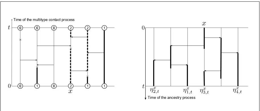
both up to time t. We should think of time for the multitype contact process as running on the opposite direction as time for the ancestry processes. This is illustrated on Figure 1.
0
0 1 00 2 1 1 0
0 00 00 2 2 1
Time of the multitype contact process
Time of the ancestry process
Figure 1: On the left, we have the multitype contact process starting from ξ0 ∈ {0, 1, 2}Z and
following a Harris constructionH. Time is increasing from bottom to top, thick lines represent the evolution of the 1’s and dashed lines represent the evolution of the 2’s. On the right, we have the ancestry process of x ∈Zfollowing It(H). Time is increasing from top to bottom. The facts that
ξ0(η1,xt) =ξ0(η2,xt) =0 andξ0(η3,xt) =2 imply thatξt(x) =2.
We now write our fundamental duality relation: for eachx ∈Z,
ξt(x) = ¨
0, if for eachn, eitherξ0(ηxn,t) =0 orηnx,t=△;
ξ0(ηnx∗(x),t), otherwise,
(2.5)
where n∗(x) =inf{n:ξ0(ηnx,t)6=0}. This can be seen at work in Figure 1. Its formal justification
(Jtγ)(s) =γ((t−s)+);Jtγis thusγran backwards and repaired so that we get a right continuous path. We then haveγ < γ′⇔ Jtγ´Jtγ′, so all maximality properties can be translated from one
space of paths to the other.
The obvious utility of (2.5) is that it allows us to relate properties of the distributions of the multitype contact process and of the ancestry processes at a fixed time. Let us state two such relations. First,
P(∀x,ξt(x)6=1) =P
∀x, eitherη∗x,t=;, or
ξ0 is equal to 0 onη∗x,t, or
ξ0(ηnx∗(x),t) =2
, (2.6)
wheren∗(x)was defined after (2.5). This will be useful for our proof of Theorem 1.1. Second, taking
ξ0=ξh(the heaviside configuration defined in the Introduction) andρtas in the Introduction,
P(|ρt|> L) =P(|sup{x :η1,xt≤0} −inf{x :η x
1,t>0}|>L). (2.7)
This will be useful in our proof of Theorem 1.3. We have now concluded Step 3.
Even though the relations of Step 3 will be extremely useful, our standard point of view will be the one of Step 2. This means that, from now on, unless explicitly stated otherwise, we will have an infinite-time Harris construction H used to jointly define, for every x ∈Z, the ancestry processes
((ηnx,t)n∈N)t≥0. Whenever we mention a function of the Harris construction, such as T(x,s)orMt(x,s), we mean to apply it to the Harris construction used to define the ancestry process.
The following is an easy consequence of the definition of the ancestry process with the ordering of paths ´ defined above.
Lemma 2.2. (i.)Let0<s<t, assume thatηx
s 6=△and T (ηx
s,s)>t. Then,ηx
t =η (ηsx,s)
t . In particular,
if T(ηsx,s)=∞, then for all s′>s we haveηx
s′=η
(ηx s,s)
s′ . (ii.)Let0≤s<t,z1, . . . ,zN∈Zand assume
ηx
i,s6=△, η (ηx
i,s,s)
∗,t =;, 1≤i<n
ηnx,s6=△,(η(η
x n,s,s) 1,t , . . . ,η
(ηx n,s,s)
N,t ) = (z1, . . . ,zN)
(that is, the first n−1ancestors of x at time s do not reach time t, but the n-th one does, with ancestors z1, . . . ,zN at time t). Then, we have(η1,xt, . . . ,ηNx,t) = (z1, . . . ,zN).
Givenx ∈Z, on{Tx=∞}, define
τ1x =inf{t≥1 :T(ηtx,t)=∞},
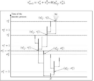
the first time after 1 at which the first ancestor of x lives forever. It is useful to think of τ1x as the result of a sequence of attempts, as we now explain and illustrate on Figure 2. Defineσ1x ≡1 and, forn≥1,
σnx+1=
(
+∞ ifσnx = +∞;
T
ηx σnx,σ
x n
otherwise. (2.8)
σx
n is thought of as the time of the n-th attempt to find a first ancestor of x that lives forever. If
(ηx
σx
1,σ
x
1) = (η1x, 1) lives forever (that is, if T
(ηx
1,1)= ∞), we haveτx
attempt succeeds. Otherwise, we must wait untilσ2x =T(η1x,1)to start the second attempt. This is
because for any t ∈(σ1x,σ2x), we have η
(ηx σx1,σ
x
1)
t = ηxt as a consequence of Lemma 2.2(i.), so in
particular(ησxx
1
, σ1x)↔(ηxt,t)and then T(ηxt,t)≤T (ηx
σ1x,σ x
1)
<∞. Next, if(ησxx
2
,σ2x)lives forever, then the second attempt succeeds and we haveτ1x =σ2x; otherwise we must wait for(ησxx
2
,σ2x)to die, and so on.
On{Tx =∞}, also defineτx
0 ≡0 and, forn≥1,
τnx+1=τnx+τ01◦θ(ητxx n,τ
x n).
Figure 2: Renewal times. We detail the attemptsσix to find the first renewal,τx1. The first ancestor process is given by the thick line. The top of the figure means that(ηxτx
3, τ
x
3)lives forever.
For the sake of readability, we will sometimes write ˜Px(
·) and ˜Ex(
·) instead of P(·|Tx = ∞) and
E(·|Tx =∞). In Proposition 1 in[15], it is shown that under ˜Px, the timesτx
n work as renewal
times for the processηx
t, that is, the (Time length, Trajectory) pairs
(τnx+1−τnx, t∈[0,τnx+1−τnx]7→ητxx n+t−η
x
τx n)
are independent and identically distributed. This follows from an idea of Kuczek ([9]) which has be-come an important tool in the particle systems literature. In our current setting, it can be explained as follows. The probability ˜Px is the original probability for the process conditioned on the event
{(x, 0)lives forever}. But(x, 0)being connected to(ητxx
1
,τ1x)and(ητxx
1
,τ1x)living forever imply that
(x, 0)lives forever, the event of the former conditioning. This and the fact that, underP, restrictions ofH to disjoint time intervals are independent yield that, under ˜Px, the shifted Harris construction
θ(ηx
τx
1,τ
x
We now list the properties of the renewal times that we will need.
Proposition 2.3. (i.)˜P0(τ0n<∞) =1∀n.
(ii.) For n≥0, let
Hn=H[0,τ0
n(H)], Hn+=θ(η 0 τ0
n
,τ0n)(H).
Given an event A on finite-time Harris constructions and an event B on Harris constructions, we have
˜
P0(H
n∈A,Hn+∈B) =P˜0(Hn∈A)·˜P0(H∈B).
(iii.) UnderP˜x, theZ-valued process ηxτx n
n≥0 is a symmetric random walk starting at x and with transitions
P(z,w) =P˜0 η0 τ0
1
=w−z
.
(i v.) There exist c,C >0such that
˜
P0 τ0 1∨M
0 τ1>r
≤C e−c r.
Except for part(ii.), the above proposition is contained in Proposition (1), page 474, of [15]((i.)
and(i v.)are explicitly on the statement of the proposition and(iii.)is a direct consequence of(i.)). Part(ii.)is an adaption of Lemma 7 in[14]to our context; since its proof also uses ideas similar to the ones of Proposition (1) in[15], we omit it.
To conclude this section, we prove some simples properties of the first ancestor process.
Remark 2.4. Every time we write events involving a random variableη that may take the value △, such as{η≤0}, we mean{η6=△,η≤0}. This applies to part(iii)of the following lemma. Also, by convention we putE(f(η)) =E(f(η);η6=△)for every function f :Z→R.
Lemma 2.5. (i.)There exist c,C>0such that, for all0≤a<b,
˜
P0(∄n:τ0
n∈[a,b])≤C e− c(b−a).
(ii.)There exists C >0such that, for all0≤s<t,
˜
E0 (η0
t)
2
−(η0s)2
≤C+C(t−s).
(iii.)There exist c,C >0such that for all l≥0,
P(|η0t|>l)≤C e−cl2/t+C e−cl.
Proof. Define on{T0=∞}, for t≥0,
τt−=sup{τ0n≤t:n∈N}, τt+=inf{τ0n≥t:n∈N}, ψt=M
ητt
−,τt−
Using Proposition 2.3(ii.)and(i v.),
Observe that the above expectation is less than 1, because there is at most one renewal in each unit interval. (2.9) is thus less than
C
since this does not depend ont, we get
˜
With (2.11), (2.12) and (2.13) at hand, we are ready to estimate
Let us treat each of the three terms separately.
˜
since, by the independence of increments between different pairs of renewals and symmetry, ˜
By (2.13), this is less than
C
Z t
s
(t−r+1)P˜0(τs+∈d r)≤C(t−s+1).
Putting this, (2.16) and (2.17) back in (2.14) completes the proof.
(iii.)Forl≥0,
P(|η0t|>l) =P(t<T0<∞,|η0t|>l) +P(T0=∞)P˜0(|η0t|>l).
The first term is less than
3
Pairs and sets of ancestries
In this section, we study the joint behavior of ancestral paths. For pairs of ancestries, we define joint renewal points that have properties similar to the ones just discussed for single renewals, and then use these properties to study the speed of coalescence of first ancestors. For sets of ancestries, we show that, givenN >0, the overall density of sites ofZoccupied by ancestors of rank smaller than or equal toN at timet tends to 0 ast → ∞.
Let us define our sequence ofjoint renewal times. Fixx,y ∈Zand on{Tx =Ty =∞}define
τ1x,y =inf{t≥1 :T(ηxt,t)=T(η y
t,t)=∞},
the first time after 1 at which both the first ancestor of x and the one of y live forever. In parallel with (2.8), defineσ1x,y ≡1 and, forn≥1,
The sequence of attempts in this case works as follows. We start asking if both(ησxx,y
1
n for any x andn. We have the following analog of Lemma 2.3:
Proposition 3.1. (i.)˜Px,y(τnx,y<∞) =1∀n,x,y.
(ii.) For n≥0, let
Hn=H[0,τxn,y(H)], Hn+=θ(0,τ
x,y n )(H).
We omit the proof since it is an almost exact repetition of the one of Lemma 2.3; the only difference is that, when looking for renewals, we must inspect two points instead of one.
We now study the behavior of the discrete time Markov chain mentioned in part(iii.)of the above proposition. Our first objective is to show that the time it takes for two ancestries to coalesce has a tail that is similar to that of the time it takes for two independent simple random walks onZto meet. This fact will be extended to continuous time in Lemma 3.3; in Section 5, we will establish other similarities between pairs of ancestries and pairs of coalescing random walks.
Lemma 3.2. (i.)For z∈Z, letπz denote the probability onZgiven by
πz(w) =P˜0,z
ηz
τ0,1z−η 0
τ0,1z=z+w
, w∈Z.
There exist a symmetric probabilityπonZand c,C >0such that
||πz−π||T V ≤C e−c|z| ∀z∈Z,
where|| · ||T V denotes total variation distance.
(ii.)There exists C >0such that, for all x,y∈Zand n∈N,
˜
Px,y ηx
τnx,y 6
=ηy
τxn,y
≤ C|xp−y|
n .
Proof. (i.) Fixz ∈Z. For simplicity of notation, we will go through the proof in the casez > 0; however, it will be clear how to treat the casez<0. Let us take two random Harris constructions
H1 and H2 defined on a common space with probability measure P, under whichH1 andH2 are independent and both have the original, unconditioned distribution obtained from the construction with Poisson processes. DefineH3as a superposition ofH1andH2, as follows. We include inH3:
•fromH1, all death marks in sites that belong to(−∞,⌊z/2⌋]and all arrows whose starting points belong to(−∞,⌊z/2⌋];
•fromH2, all death marks in sites that belong to(⌊z/2⌋,∞)and all arrows whose starting points belong to(⌊z/2⌋,∞).
Then, H3 has same law as H1 and H2. We will write all processes and times defined so far as functions of these Harris constructions: fori∈ {1, 2, 3}, we may take
η(nx,t,s)(Hi)forx ∈Z, n∈N, s<t;
M(tx,s)(Hi)andT(x,s)(Hi)forx ∈Z, s<t;
τ(nx,y)(Hi)on{Tx(Hi) =Ty(Hi) =∞}, for x,y∈Z, n∈N,
as defined before and nothing new is involved. On the event{T0(H1) =Tz(H2) =∞}, define
˜
τ0,z=inf{t≥1 :T(η0t(H1),t)(H1) =T(ηzt(H2),t)(H2) =∞}.
Our definition of ˜τ0,z is similar to the one of first joint renewal time of two first ancestor processes.
However, for ˜τ0,z, we follow a different Harris construction for each ancestor process. We can also think of ˜τ0,z as the result of a “sequence of attempts”, and define corresponding stopping times similar to the ones illustrated on Figure 2. The same proof that establishes Proposition 3.1(i v.)can be repeated here to show that there existc,C >0 such that
P T0(H1) =Tz(H2) =∞, ˜τ0,z∨Mτ0˜0,z(H 1)
∨Mτz˜0,z(H
2)>r
Now define
X0,z =
(
ηz
τ0,1z(H3)(H
3)
−η0
τ0,1z(H3)(H
3) if T0(H3) =Tz(H3) =
∞
△ otherwise;
Y0,z =
¨
ηz
˜ τ0,z(H
2)−η0 ˜ τ0,z(H
1) ifT0(H1) =Tz(H2) =∞,
△ otherwise.
Note that
πz(·) =P(X0,z=z+· |X0,z6=△), (3.2)
whereπz is defined in the statement of the lemma. Also define
π(·) =P(Y0,z=z+· |Y0,z6=△). (3.3)
By the definition ofY0,zfrom independent Harris constructions,πis symmetric and does not depend onz. To conclude the proof, we have two tasks. First, to show thatX0,z=Y0,z with high probability whenzis large. Second, to show that this implies that, whenzis large,||πz−π||T V is small.
Letκbe as in (2.1) and definet∗=z/3κ. Consider the events
L1={Mt0∗(H1)∨Mtz∗(H2)<z/2},
L2={T0(H1)∧Tz(H2)<t∗},
L3=
¨
T0(H1) =Tz(H2) =T0(H3) =Tz(H3) =∞,
τ0,1z(H3)<t∗, ˜τ0,z<t∗
«
.
On L1, we have {(x,t) : 0 ≤ t ≤ t∗, (0, 0) ↔ (x,t)inH1} ⊂ (−∞,⌊z/2⌋]×[0,t∗]. Since the
restriction ofH1 to(−∞,⌊z/2⌋]×[0,t∗]coincides with the restriction of H3 to the same set and similar considerations apply toH2 and the set(⌊z/2⌋,∞)×[0,t∗], we get that, onL1,
η0n,t(H1) =η0n,t(H3), ηzn,t(H2) =ηzn,t(H3), ∀n∈N, 0≤t≤t∗. (3.4)
We now claim that, if the eventL := (L1∩ L2)∪(L1∩ L3)occurs, thenX0,z =Y0,z. To see this, assume first that L1∩ L2 occurs. Then, by the definition of L2, we either have T0(H1) < t∗ or
Tz(H2) < t∗. In any case we have Y0,z = △and, also using (3.4), we either get T0(H3) < t∗ or
Tz(H3)<t∗, soX0,z=△. Now assumeL1∩ L3 occurs. Define
t1=τ˜0,z, a1=η0t
1(H
1), b
1=ηzt1(H
2);
t2=τ0,1z(H3), a2=η0t
2(H
3), b
2=ηzt2(H
3).
By (3.4) and the fact that t1,t2≤ t∗, if we show that t1 = t2, we geta1 = a2 and b1 = b2, hence
Y0,z=b1−a1=b2−a2=X0,z. Assume t1≤t2. Again by (3.4) and the fact thatt1≤t∗, we have
η0t
1(H
3) =
η0t
1(H
1) =a
1, ηzt1(H
3) =
ηzt
1(H
2) = b
1. (3.5)
The definition of t1 implies that T(a1,t1)(H1) = T(b1,t1)(H2) = ∞, and then we obviously have (a1,t1)↔ Z× {t∗} in H1 and(b1,t1) ↔ Z× {t∗} in H2; since we are assuming L1 occurs, the paths that make these connections are also available inH3. This gives
We now use (3.5), (3.6) and the definition ofa2,b2 in Lemma 2.2(i.)to conclude that
3) is defined as the infimum over all times t
≥ 1 that satisfy T(η0t,t)(H3) = T(ηzt,t)(H3) =∞, we see from (3.5) and (3.8) that t2 ≤ t1, so t2 = t1. A similar set of arguments
show that t2≤t1 impliest1=t2. This completes the proof of the claim.
Now note that the eventLcis contained in the union of:
{Mt0∗(H1)>z/2},{Mtz∗(H2)>z/2},
{t∗<T0(H1)<∞},{t∗<T0(H3)<∞},{t∗<Tz(H2)<∞},{t∗<Tz(H3)<∞},
{T0(H1) =Tz(H2) =∞, ˜τ0,z>t∗},{T0(H3) =Tz(H3) =∞,τ0,1z(H3)>t∗}.
Using our choice of t∗, (2.1), (2.3), Proposition 3.1(iii.)and (3.1), the probability of any of these events decreases exponentially withz.
We thus haveP(X0,z6=Y0,z)≤C e−cz, so
where we have applied (3.2) and (3.3) in the second equality and (3.9) in the last two inequalities. We have P(X0,z 6= △) = P(T0(H3) = Tz(H3) = ∞) and P(Y0,z 6= △) = P(T0(H1) = Tz(H2) =
∞), and these probabilities are bounded away from zero uniformly in z by (2.2). We thus get
Using Proposition 3.1(iii.) and translation invariance, we see that under ˜Px,y, Xx,y
n is a Markov
chain that starts at y−x and has transitions
˜
In particular, 0 is an absorbing state.(ii.)follows from Theorem 6.1 in Section 6. Here, let us ensure that the four conditions in the beginning of that section are satisfied byπz andπ. Conditions (6.1)
and (6.4) are already established. Condition (6.2) is straightforward to check and (6.3) follows from (3.1) and Proposition 3.1(i v.).
We now want to define a random timeJx,y that will work as a “first renewal after coalescence” for the first ancestors ofx and y, a time after which the two processes evolve together with the law of a single first ancestor process. Some care should be taken, however, to treat the cases in which the ancestries of x or of y die out. With this in mind, we put
for someC >0.
The claim is a direct consequence of this equality.
Lemma 3.4. There exist c,C>0such that, for any x,y∈Z,N≥1and t≥0,
P(Tx,Ty >t,(η1,xt, . . . ,ηNx,t)6= (η1,yt, . . . ,ηNy,t))≤C eC N−c t+C|xp−y| t .
Proof. There existsδ >0 such that, given a finite setA⊂Z, we have
P(TA<∞)> δ|A|. (3.11)
We can for instance takeδas the probability of a particle dying out before having any children, an observe that this occurs independently for different sites. Define
with the convention inf;=∞. Then, ˜σN is a stopping time and{σN>t}={σ˜N <∞}. Using this,
(3.11) and the Strong Markov Property, we have
P(t<T0<∞)≥ X
A⊂Z, 0<#A≤N
P(σ˜N <∞, η∗0, ˜σN =A)·P(T
A< ∞)
≥δN X
A⊂Z, 0<#A≤N
P(σ˜N<∞, η0∗, ˜σN =A) =δ
NP(˜
σN<∞) =δNP(σN >t).
We then haveP(σN >t)≤δ−NP(t<T0<∞); also using (2.3), we obtain
P(σN >t)≤C1eC2N−c1t. (3.12)
for someC1,c1,C2>0.
Let x,y ∈Z; assume that Tx = Ty =∞and Jx,y +σN ◦θ(ηxJx,y,Jx,y)≤ t. This means that first,
(ηx)and(ηy)have the first joint renewal at some space-time point(ηx
Jx,y,Jx,y) = (η
y
Jx,y,Jx,y)with Jx,y ≤t, and second, that the ancestry process of(ηJxx,y,Jx,y)never has less thanN elements after
timet. We must then havez1, . . . ,zN ∈Zsuch that
η0n,t−Jx,y◦θ(ηJxx,y,Jx,y) =η0n,t−Jx,y◦θ(η
y
Jx,y,Jx,y) =zn, 1≤n≤N.
Lemma 2.2 then implies thatηxn,t=ηny,t=zn, 1≤n≤N, and we have thus shown that
{Tx =Ty =∞, Jx,y+σN◦θ(ηJxx,y,Jx,y)≤t}
⊂ {Tx =Ty =∞, (η1,xt, . . . ,ηNx,t) = (η1,yt, . . . ,ηNy,t)}.
Then,
P(Tx =Ty=∞, (η1,xt, . . . ,ηNx,t)6= (η1,yt, . . . ,ηNy,t) )
≤P(Tx =Ty =∞, Jx,y +σN◦θ(η1,xJx,y,Jx,y)>t) ≤P(Jx,y >t/2) +P(σN◦θ(η1,xJx,y,Jx,y)>t/2
Tx =∞)
≤ C|xp−y|
t +C e
C N−c t,
where in the last inequality we used Lemma 3.3(i.)in the first term and Lemma 3.3(ii.)and (3.12) in the second.
Finally, we have
P(Tx,Ty >t,(η1,xt, . . . ,ηNx,t)6= (η1,yt, . . . ,ηNy,t))
≤P(t<Tx <∞) +P(t <Ty<∞) +P(Tx =Ty =∞,(η1,xt, . . . ,ηNx,t)6= (η1,yt, . . . ,ηNy,t))
≤2C e−c t+C eC N−c t+ C|xp−y| t ≤C e
C N−c t+C|x−y| p
t .
Proposition 3.5. There exist C,γ >0such that, for any N ≥1and t≥0,
Proof. Fix a realt ≥0 and a positive integerl withl>N. DefineΓ ={0, . . . ,l−1}and
that is, for all sites in Γthat have non-empty ancestry at time t, the firstN terms of the ancestor sequence at timet must coincide. We can use Lemma 3.4 to bound the probability ofΛc:
P(Λc)≤ X
and the unions are disjoint, (3.15) is equal to
We now putl=t19; we have thus obtained
P 0∈ {ηxn,t:x ∈Z, 1≤n≤N} ≤
N
t1/9 +
C N t4/9
t1/2 +C N t
1/3eC N−c t
∧1
≤ N
t1/9 + C N
t1/18 + (C N t
1/3eC N−c t) ∧1.
The first two terms are already in the form we want, and it is straightforward to show that, for some
C′>0, we have(C N t1/3eC N−c t)∧1≤C′N/t for allN,t.
4
Extinction, Survival and Coexistence
In this section we prove Theorems 1.1 and 1.2. Our three key ingredients will be a result about extinction under a stronger hypothesis (Lemma 4.1), an estimate for the edge speed of one of the types when obstructed by the other (Lemma 4.2) and the formation of “descendancy barriers” for the contact process onZ(Lemma 4.3).
We recall our notation from the Introduction: the letters ξ andη will be used for the multitype contact process and the ancestry process, respectively. Throughout this section, in contrast with the rest of the paper, Harris constructions and statements related to them, such as “(x,s) ↔ (y,t)”, refer to the construction forξrather than the one forη.
Lemma 4.1. For the process(ξt)with initial stateξ0such that there exists A>0such thatξ0(x) =2 for all x with|x| ≥A, the1’s almost surely die out, i.e. almost surely there exists t such thatξt(x)6=
1∀x.
Proof. Using (2.6), for anyt0>0 we have
P(∃t:∀x,ξt(x)6=1)≥P(∀x,ξt0(x)6=1) =P
∀x, eitherη∗x,t
0=;, or
ξ0 is equal to 0 onη∗x,t0, or
ξ0(ηnx∗(x),t
0) =2
≥P
∀x, eitherη∗x,t
0=;or
η1,xt
0∈(−A,A)
c
≥1−
A X
i=−A
P(∃x : η1,xt
0=i).
By (3.5) each of the probabilities in the last sum converges to 0 ast0→ ∞.
Lemma 4.2. Fixβ >0. For anyε >0, there exists K>0such that, ifξ0=ξH=1(−∞,0]+2·1(0,∞),
then
P(sup{x:ξt(x) =1} ≤K+βt ∀t)>1−ε.
Proof. ForK>0, consider the events
An = {ξn(x) =1 for somex ≥K/2+βn/2},
n∈ {0, 1, 2, . . .}. Now, using Lemma 2.5(iii.),
a unit time interval; by a comparison with a multiple of a Poisson random variable as in (2.1), this
occurs with probability smaller thanC e−c(K/2+βn/2)for somec,C >0, soP(∪nBn)≤PnP(Bn)K−→→∞0 as well. This givesP(∩n(Acn∩Bnc))→1 asK→ ∞, and to conclude the proof note that on∩n(Acn∩Bnc), the set{(x,t):ξt(x) =1}is contained in{(x,t):x<K+βt}.
Forρ > 0, define V(ρ) ={(x,t) ⊂Z×[0,∞) :−ρt ≤ x ≤ ρt}. We say that site 0 forms a ρ -descendancy barrier (according to the Harris constructionH) if
(D1)for anyx,y∈Zand t≥0 with(x, 0)↔(y,t)and(y,t)∈V(ρ), we have(0, 0)↔(y,t);
(D2)for any x,y ∈Zwith opposite signs and t ≥0 such that(x, 0)↔ (y,t), we have(0, 0) ↔ (y,t).
Say thatx ∈Zforms aρ-descendancy barrier if the origin forms aρ-descendancy barrier according toθ(x, 0)(H).
Lemma 4.3. For anyε >0, there existsβ,K>0such that
P(∃x∈[0,K]:x forms aβ-descendancy barrier)>1−ε.
The proof is in[2]; see Proposition 2.7 and the definition of the eventH2 in page 10 of that paper.
This can be verified by looking at the generator of the multitype contact process. It is an attractive-ness property: defining the partial orderξ′≺ξ′′⇔ {ξ′=1} ⊃ {ξ′′=1},{ξ′=2} ⊂ {ξ′′=2}, the above lemma says that the set{(ξ′,ξ′′):ξ′≺ξ′′}is invariant under the coupled dynamics we are considering.
Lemma 4.5. Assume at least one site is occupied by a1inξ0and let K ∈N.
(i.) If conditions (A) and (B) of Theorem 1.1 are satisfied, then almost surely there exist (random) L′,a1,a2∈Zwith L′>0,a1<−L′,a2>L′such that
(A′) ξ1(x)6=1∀x∈/[−L′,L′];
(B′) #{x ∈(−∞,L′]:ξ1(x) =2}=#{x ∈[L′,∞):ξ1(x) =2}=∞; (C′) ξ1(x) =2∀x∈[a1−K,a1]∪[a2,a2+K].
(ii.)Assume condition(A)of Theorem 1.1 is satisfied but condition(B)is not (say, with finitely many 2’s in[0,∞)) and, for a given a∈Z, we haveξ0(a) =1. Then, with positive probability,
(A′′) ξ1(x) =1∀x∈[a,a+K]; (B′′) ξ1(x)6=2∀x>a+K.
(iii.) Assume the hypotheses of Theorem 1.2 are satisfied and, for given b,c ∈Zwith b<c, we have
ξ0(b) =i, ξ0(c) =j, where{i,j}={1, 2}. Then, with positive probability,
(A′′′) ξ1(x)6= j∀x ∈(−∞,c−K); (B′′′) ξ1(x) =i∀x ∈[c−K,c); (C′′′) ξ1(x) = j∀x ∈[c,c+K); (D′′′) ξ1(x)6=i∀x ∈[c+K,∞).
Proof of Theorem 1.1. We first prove that, if conditions(A)and(B)in the statement of the theorem are satisfied, then the 1’s almost surely become extinct. Fixε >0. As in Lemma 4.3, chooseβ,K1
corresponding toε, then as in Lemma 4.2, chooseK2corresponding toεandβ. LetK=K1+K2+2R. Using Lemma 4.5(i.)with this value ofK and relabeling time so as to start looking at the process at time 1, we may assume that there exista1,a2,L′such that (A′),(B′)and(C′)are satisfied byξ0
(rather than byξ1).
Let (ξ1t),(ξ2t),(ξ12t ) and (ξ21t ) be realizations of the multitype contact process all built using the same Harris construction as the original process(ξt)and having initial configurations
ξ10=1(a1,a2)+2·1[a1−K,a1]+2·1[a2,a2+K];
ξ20=1(a
1,a2)+2·1(a1,a2)c;
ξ120 =1(−∞,a
2)+2·1[a2,∞);
ξ210 =2·1(−∞,a1]+1(a1,∞).
By a series of comparisons and uses of the previous lemmas, we will show that inξ1, the 1’s become extinct with high probability. An application of Lemma 4.4 to the pairξ1,ξthen implies that inξ, the 1’s become extinct with high probability.
Define the events