Classification of Imbalanced Land-Use/Land-Cover
Data Using Variational Semi-Supervised Learning
Tjeng Wawan Cenggoro
∗†, Sani M. Isa
‡, Gede Putra Kusuma
‡, and Bens Pardamean
†‡ ∗Computer Science Department, School of Computer Science, Bina Nusantara University,Jakarta, Indonesia 11480
†Bioinformatics and Data Science Research Center, Bina Nusantara University, Jakarta, Indonesia 11480
‡Computer Science Department, BINUS Graduate Program - Master of Computer Science, Bina Nusantara University, Jakarta, Indonesia 11480
e-mail: [email protected], [email protected], [email protected], [email protected]
Abstract—Classification of Land Use/Land Cover (LULC) data is a typical task in remote-sensing domain. However, because the classes distribution in LULC data is naturally imbalance, it is difficult to do the classification. In this paper, we employ Variational Semi-Supervised Learning (VSSL) to solve imbalance problem in LULC of Jakarta City. This VSSL exploits the use of semi-supervised learning on deep learning model. Therefore, it is suitable for classifying data with abundant unlabeled like LULC. The result shows that VSSL achieves 80.17% of overall accuracy, outperforming other algorithms in comparison.
Index Terms—Variational Autoencoder, Variational Semi-Supervised Learning, Remote Sensing, Imbalanced Learning
I. INTRODUCTION
In remote-sensing domain, classification of Land Use/Land Cover (LULC) data plays an important role. A good LULC classification can monitor changes in the use of land. For instance, we can monitor the growth of urban area in a certain time range. However, LULC data is typically difficult for classification task. The main reason for this fact is that LULC tends to be imbalance, which means that there are classes which size are much greater than other classes.
Imbalance data is known to cause a poor classification result when it is classified by standard machine learning classifier. A classifier trained on imbalance data often classifies minority class poorly. In contrast, the classifier usually has a high prediction accuracy for majority class [1]. There are various researches proposing methods to solve imbalance-data problem. These methods are called as imbalanced learning by the community.
Among the methods for imbalanced learning, methods that based on Semi-Supervised learning are promising to be applied in remote-sensing domain. Semi-Supervised learning has been studied in several research of imbalanced learning [2], [3]. The main idea of Semi-Supervised learning for imbalanced learning is to exploit unlabeled data to help classifier learn from imbalance labeled-data. This idea is well-suited for remote-sensing domain as unlabeled remote-sensing images are abundant.
In this paper, we study on how to apply Variational Semi-Supervised Learning (VSSL) [4] to solve imbalance-data
prob-lem in LULC classification of urban area. The LULC data used in this paper is collected from Jakarta City, Indonesia.
II. RELATEDWORKS
To the best of our knowledge, the work by Bruzzone & Serpico [5] is the earliest work with focus in imbalanced-learning in remote-sensing. In order to solve the imbalance-data problem, they propose method to train neural network (NN) which is able to switching cost function in certain condition. Firstly, the neural network is trained using a special cost-function for imbalanced-learning. This objective function is derived from standard Mean Square Error (MSE), and calculated as E = PMl=1 1
nM
PM
k=1 Pnl
l=1[t
(l)
k −ok(x
(l)
k )]
2.
Here,M is the total number of classes. t(kl) andok(x(kl))are
elementkof one-hot vector for true and predicted classlgiven inputx(kl).Elis the error of classl. With this modification, an
increase of MSE of minority classes can be avoided in early stage of training. After the MSE of each class is lower than a predetermined threshold value T, the cost is switched to standard MSE. In this work, they use remote sensing images that are captured by thematic mapper sensor attached to an aircraft. The bands used are the bands with similar wavelength range to band number 1, 2, 3, 4, 5, and 7 of Landsat.
Another study that focuses on imbalanced-learning in remote-sensing is performed by Waske et al. [6]. They propose to use bootstrap aggregating (Bagging) on an ensemble of Support Vector Machines (SVM). For the purpose of tackling the imbalance-data problem, each of the SVM is fed with a balanced sub-dataset. This sub-dataset is obtained by random downsampling from the whole dataset. The remote-sensing images used are high resolution images that are captured by SPOT satellite.
III. MATERIALS ANDMETHODS
A. Study Area
LULC is dominated by urban areas. Thus, the collected LULC data is imbalance.
B. Dataset Construction
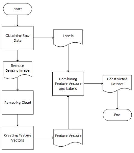
The processes flow of dataset construction in this research is illustrated in Fig. 1. The first step in this process is to obtain raw data necessary for constructing dataset. The re are two type of raw data collected in this researh, remote-sensing image and labels for each pixels in the remote-sensing image. The remote-sensing image collected is downloaded from [7], which is captured by Landsat 7 satellite. The image we choose is image with entity ID of LE71220642000258SGS00. This image is taken from WRS-2 path 122 and row 64. The date when this image is captured is September 14, 2000. Our reason for choosing this image is because the labels we are able to obtain is collected from year 2000, thus we have to use image within the year.
Fig. 1: Flows of Dataset Construction
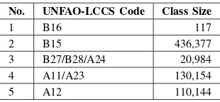
For the labels of the data, we obtain it on December 5, 2015 fromBadan Informasi Geospasial(BIG), the Indonesian Geospatial Information Agency [8]. The labels have thirteen different classes, based on Indonesian National Standard of Land Cover Classification [9]. We decide to group the classes based on United Nation Food and Agriculture Association Land Cover Classification System (UNFAO-LCCS) [10]. The grouping is shown in Table I.
After obtaining the raw data, further process is needed for the remote-sensing before it can be combined with the labels to form desired dataset for this research. Those additional process are removing cloud and creating feature vector. The cloud removal process is necessary as the pixels that are covered by the cloud is invalid to be classified to any LULC class. The
TABLE I: LULC classes grouping
No.
UNFAO-LCCS Code
Class Name
BSN Class Name
1 B16 Bare Areas Shelf
2 B15 Artificial Surfaces and Associated Areas Residence
3 B27/B28/ A24
Artificial/Natural Waterbodies, Snow, and Ice; Natural and Semi-Natural Aquatic or Regularly Flooded Vegetation
Lake Dam River Swamp
4 A11/ A23
Cultivated and Managed Terrestrial Ar-eas; Cultivated Aquatic or Regularly Flooded Areas
Field Croplands Plantation
5 A12 Natural and Semi-Natural Vegetation
Reeds, savannas, and grasslands Wetland Dry forest Shrubs
cloud removal technique we used is the technique proposed by Zhu et al. [11].
After we remove all pixels covered by cloud, we form feature vectors from the remote-sensing image. This process is essential so that the dataset can be read by classifier algorithm. We choose to form the feature vectors by taking 3x3 pixels of Band number 1, 2, 3, 4, 5, and 7 of the remote-sensing image, as depicted in Fig. 2. The gray pixel in Fig. 2 represent pixel which will be attached to labels we obtained in previous process.
Fig. 2: Illustration of single feature vector construction
To complete the process of dataset construction, we combine the constructed feature vectors with the corresponding labels. The classes distribution of the constructed dataset is shown in Table II. We can see that the distribution of classes in labeled dataset is imbalance, with class B15 dominating the dataset.
TABLE II: Class Distribution of labeled dataset
No. UNFAO-LCCS Code Class Size
1 B16 117
2 B15 436,377
3 B27/B28/A24 20,984
4 A11/A23 130,154
5 A12 110,144
of the employed VSSL model hyperparameters and also for the early stopping condition. The testing dataset is used for assessing and comparing the performance of each algorithm in our experiment. We split our dataset by ratio of 6:2:2 for the training, validation, and testing dataset respectively. In splitting the dataset, we keep the ratio of the training, validation, and testing dataset class distribution to be similar to the original dataset.
For the unlabeled dataset, we collect it from seven other Landsat 7 remote-sensing images. These images is taken from area nearby the image for labeled dataset. Table III lists images we choose for unlabeled dataset. We decide to limit the size of unlabeled data by two times of the labeled dataset size. This limitation is needed so that the VSSL model we use can run in reasonable computation time. To obtain unlabeled data with such size, we sample it randomly from the images listed in Table III.
TABLE III: Class Distribution of labeled dataset
No. Entity ID WRS-2
Path
WRS-2 Row
Year Captured
1 LE71170662002292DKI00 117 66 2002 2 LE71180652003142EDC00 118 65 2003 3 LE71190652000253SGS00 119 65 2000 4 LE71200652003140EDC00 120 65 2003 5 LE71210652003019SGS00 121 65 2003
6 LE71220652001356SGS00 122 65 2001 7 LE71230642002142SGS01 123 64 2002
C. Variational Autoencoder
Variational Autoencoder (VAE) [12] is a variant of au-toencoder which concept is based on variational bayesian inference. Similar to traditional autoencoder, VAE also tries to reconstruct input x by into xˆ. The difference of VAE from other autoencoder variants is that its latent variable z
is instead produced by sampling from distribution pθ(z|x).
VAE generates xˆ from z by sampling from a distribution
pθ(x;g(z)) = pθ(x|z). Because calculating pθ(z|x) is
in-tractable, VAE instead computes q(z|x) as approximation of
pθ(z|x) using variational inference. In the view of
Autoen-coder, the q(z|x) and pθ(x|z) can be considered as encoder
and decoder function respectively.
In contrast to traditional autoencoder—which can be trained by using standard objective function—VAE can only be trained by using variational lower boundL(q) =Ez∼q(z|x)pθ(z, x) +
DKL(q(z|x)|pθ(z))≤pθ(x). Here,DKL is Kullback-Leibler
Divergence [13].
The variational lower bound is normally not differentiable due to its stochastic function q(z|x). However, VAE can-not be trained if its objective function is can-not differentiable. To address this issue, Kingma and Welling [12] propose reparameterization trick to solve this problem. For instance, if q(z|x) = N(µ, σ2), reparameterization trick calculates
z=µ+σǫ instead of samplingz fromq(z|x). ǫis sampled from distributionN(I,0).µandσare estimated using neural network. This approach allows gradient to flow through z
and thus enables VAE to be trained. Figure 3 illustrates VAE process with Gaussian distribution as the distribution ofz.
Fig. 3: Illustration of VAE using Gaussian distribution
D. Variational Semi-Supervised Learning
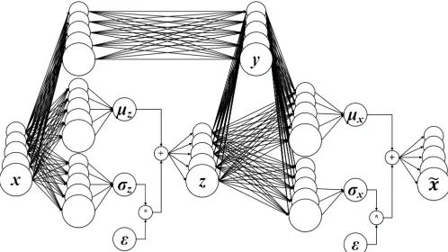
Variational Supervised Learning (VSSL) is a Semi-Supervised Learning framework for deep generative model introduced by Kingma et al. [4]. VSSL is built by stacking a standard Variational Autoencoder (VAE) [12] and a modified version of VAE called as M2 VAE (The standard VAE is called as M1 VAE when VSSL is introduced).
M2 VAE is the core concept of VSSL, which is what makes VSSL is able to learn from labeled and unlabeled data. Similar to M1 VAE, M2 VAE also learns its latent variable z by reconstructing its input x to xˆ as shown in Figure 4. The difference is thatxin M2 VAE is generated from class vectory
in addition toxas in M1 VAE.xˆin M2 VAE is also generated from y in addition to z. During training, the class vector y
comes from the label of labeled data. For unlabeled data,y is generated fromzas depicted in Figure 4. This enables VSSL to learn from both labeled and unlabeled data simultaneously. When predicting, VSSL generates labely from x.
E. Experimental Result Analysis
To analyze result in this paper, we choose to use confusion matrices and performance measurement based on it: user’s accuracy (UA), producer’s accuracy (PA), overall accuracy, and kappa coefficient. We decide to use these measurements as they are widely used to measure performance in remote-sensing domain [14], [15], [16]. Presenting the results on confusion matrices also enable us to assess the balancing effect of an imbalanced-learning.
The producer’s accuracy is calculated as PU i =xii/ xi+,
where xii is the number of correctly predicted data-points
Fig. 4: Illustration of M2 VAE using Gaussian distribution
x+i is the number of data-points that classified as classi. The
overall accuracy is then calculated as Eq 1. Here xij is the
number of data-points of classi that are predicted as classj,
q is the number of classes in dataset.
Pc=
Σqi=1xii Σqi=1Σqj=1xij
(1)
For kappa coefficient, it is calculated as Eq. (2). Kappa coefficient measures the differences between observed agree-ment and expected agreeagree-ment by matching the chances be-tween ground-truth data and predicted data. The bigger kappa coefficient value means the better a classifier performs than random guess.
ˆ
k=(
Pq i=1
Pq
j=1xij)Pqi=1xii−Pqi=1xi+x+i (Pqi=1Pqj=1xij)2−Pqi=1xi+x+i
(2)
IV. RESULTS ANDDISCUSSION
A. Experimental Setting
Before testing the performance of the VSSL model, we need to set several settings and hyperparameters in the model. For activation functions in each neurons in the model, we choose to use Rectified Linear Units (ReLU) [17], [18]. We choose ReLU because it allows error gradients to flow without vanishing. Thus, ReLU performs better than other activation function when applied in multilayer architecture.
For the optimization method we use in the VSSL model, we choose Adam [19]. Adam has been proven by by Kingma et al. [19] to perform equal or better than other stochastic gradient descent (SGD) variant such as Adagrad [20], Adadelta [21], and SGD with Nesterov momentum [22]. We set Adam hyperparameters η = 0.001, β1 = 0.9, and β2 = 0.999. The value of η is chosen as 0.001 because when we tried to use biggerηvalue for the VSSL model, all of the neurons are died (always gives 0 output). This is happens due to the nature of ReLU when applied with excessive learning rate.
To set the number of neurons of M1 and M2 VAE in the VSSL model, we run a pre-experiment accordingly. The neurons number for testing is set to 200 based on the best
result in Table IV. We use Gaussian distribution as VAE distribution function in this pre-experiment.
We also run a pre-experiment in deciding distribution func-tion to be used in M1 and M2 VAE in the employed VSSL model. Based on the pre-experiment result in Table V, we decide to use Gaussian distribution as the VAE distribution function fro the VSSL model. For this pre-experiment, we use 200 neurons in M1 and M2 VAE.
TABLE IV: Pre-experiment result on VSSL model neurons number setting
No. #Neurons Validation Accuracy Validationκˆ
1 50 79.64% 0.616
2 100 79.80% 0.620
3 200 80.17% 0.625
4 300 80.11% 0.623
5 400 80.14% 0.624
6 500 80.02% 0.622
TABLE V: Pre-experiment result on VSSL model VAE distri-bution function setting
No. Dist. Function Validation Accuracy Validationκˆ
1 Gaussian 80.17% 0.625
2 Laplace 80.06% 0.625
3 Bernoulli 78.24% 0.587
For the experiment, we choose several algorithms alongside the VSSL model to run. The result of each algorithm is then compared. In total, we selected five different algorithms, including the VSSL model, to be tested in this experiment.
The first algorithms we choose are the algorithm proposed by Bruzzone & Serpico [5] This algorithm is chosen because it has been proven to perform well in imbalance remote-sensing data, thus are ideal to be compared in our experiment. The NN employed in this algorithm for the experiment uses one hidden layer with 200 neurons. The hidden layer is set to the same value as the employed VSSL model so that the comparison is fair. The learning rate and cost-threshold T are set to 0.1 and 0.097. The value of T is set to 0.097 because the overall accuracy error suddenly decreased significantly when all of the class error goes beyond this value when the technique applied to our dataset.
The second algorithm to use is the algorithm proposed by Waske et al. [6]. This algorithm is also chosen because it has shown a good performance on imbalance remote-sensing data. For this algorithm, we set the number of SVM instances to ten. As for the kernel of SVM instances, we choose sigmoid kernel. This kernel is chosen because it performs better than other kernel on our dataset.
SMOTE algorithm we use, we set the parameterN differently based on the size of each class. This setting is done so that each of the minority class has a same size to majority class. The setting of N for class B16, B27/B28/A24, A11/A23, and A12 are 384686.57%, 2059.78%, 334.99%, and 391.62%. For the parameter k, we set it to 5.
B. Experimental Results and Discussion
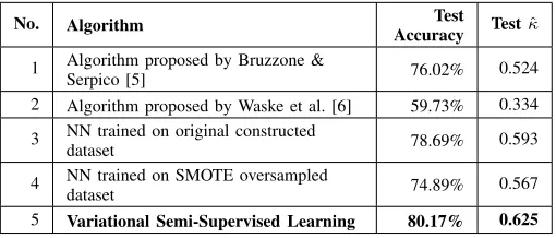
The summary of our experiment results are shown in Table VI. From this table, we can see that VSSL achieves the best overall accuracy outperforming other algorithms We also provide the result of each algorithm in confusion matrix. From these confusion matrices, we can see the effect of imbalance-learning in balancing the result of each class.
TABLE VI: Summary of the experiment result
No. Algorithm Test
Accuracy Testˆκ
1 Algorithm proposed by Bruzzone &
Serpico [5] 76.02% 0.524
2 Algorithm proposed by Waske et al. [6] 59.73% 0.334
3 NN trained on original constructed
dataset 78.69% 0.593
4 NN trained on SMOTE oversampled
dataset 74.89% 0.567
5 Variational Semi-Supervised Learning 80.17% 0.625
TABLE VII: Confusion matrix of NN trained on original constructed dataset
B15 3 80152 426 8760 4085 85.79% B27/
B28/ A24
0 76 2341 406 269 75.71%
A11/
A23 9 4370 972 13193 4293 56.22% A12 10 1315 432 3287 12660 71.51% PA 0.00% 93.29% 56.13% 51.44% 57.71% 78.69%
The confusion matrices of NN trained on original con-structed dataset is presented in Table VII. We can see from these tables that, without any imbalanced-learning, the most dominant class B15, has a big gap in producer’s accuracy compared to other minority classes. The gap is especially sever for the smallest class B16.
When trained on SMOTE upsampled dataset, NN receives a better balance in their producer’s accuracy as shown in Table VIII. Three minority classes, B16, B27/B28/A24 and A12, receive a significant performance gain in their producer’s accuracy compared to the results without any imbalanced-learning. However, as a consequence, the producer’s accuracy of majority class is greatly decreased from the no-imbalanced-learning results. It is also noticeable that for class A11/A23,
TABLE VIII: Confusion matrix of NN trained on SMOTE oversampled dataset
B15 0 71398 177 4583 1893 91.48% B27/
B28/ A24
0 972 3302 1813 985 68.49%
A11/
A23 2 7774 402 11576 2209 52.78% A12 3 5794 290 7660 16829 55.04% PA 77.27% 83.11% 79.17% 45.14% 76.72% 74.89%
TABLE IX: Confusion matrix of algorithm proposed by Waske et al. [6]
B15 0 59516 516 8509 2919 82.67% B27/
B28/ A24
7 1454 2629 2438 2295 29.80%
A11/
A23 1 14647 406 7299 3787 27.92% A12 0 9211 607 6810 12784 43.47% PA 63.64% 69.27% 63.03% 24.86% 58.28% 59.73%
TABLE X: Confusion matrix of algorithm proposed by Bruz-zone & Serpico [5]
Ground Truth
B15 2 82035 672 12180 4881 82.22% B27/
B28/ A24
0 148 1918 425 228 70.54%
A11/
A23 13 2231 855 7712 3817 57.72%
A12 0 1487 726 5235 13001 63.30% PA 31.82% 95.49% 45.98% 30.07% 59.27% 76.02%
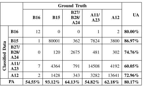
TABLE XI: Confusion matrix of VSSL
B15 1 80001 362 7824 3800 86.97% B27/
B28/ A24
0 120 2675 481 302 74.76%
A11/
A23 7 4364 791 14508 4192 60.05% A12 2 1428 343 3282 13641 72.96% PA 54.55% 93.12% 64.13% 54.82% 62.18% 80.17%
The result produced by the algorithm proposed by Waske et al. [6] shows a similar pattern to the NN trained on SMOTE upsampled dataset. However, the producer’s accuracy of all classes is generally dropped significantly compared to NN trained on SMOTE upsampled dataset. Only class B16 that still receives a good producer’s accuracy. This result is presented in Table IX.
Meanwhile, the algorithm proposed by Bruzzone & Serpico [5] is able to increase producer’s accuracy of class B16, B15, and A12 compared to NN trained on original con-structed dataset. On contrary, the producer’s accuracy of class B27/B28/A24 and A11/A23 are decreased.
Compared to other algorithms discussed so far, VSSL achieves the best overall accuracy. Not only that, VSSL is also able to balance the producer’s accuracy of minority classes. This result is presented in Table XI.
V. CONCLUSION ANDFUTUREWORKS
In this research, we study how to learn from imbalance LULC data that taken from urban area. Because of the abun-dance of remote-sensing image, we study on how to employ semi-supervised learning for tackling imbalance-data problem. To be specific, we use Variational Semi-Supervised Learning (VSSL) model in this research.
The result of our experiment proofs that VSSL can out-perform other compared algorithm with overall accuracy of 80.17%. This accuracy is 1.48% better than the second best overall accuracy (standard NN trained on original constructed dataset). It is also 4.15% better than the best imbalanced-learning technique in comparison (algorithm proposed by Bruzzone & Serpico [5]).
For the next works, it is promising to use a model with more processing layer than the VSSL model employed in this research. Model with more layers has been known to perform better in the deep-learning community, as long as the model can escape from overfitting and vanishing gradient problem.
Another promising approach is to design a special cost function for VSSL to tackle imbalance-data problem as studied by Bruzzone & Serpico [5]. However, this approach may diminish the model capability to generalize because of its assumption that the data is imbalance.
ACKNOWLEDGMENT
We would like to acknowledge supports for this project from Bioinformatics and Data Science Research Center, Bina Nusantara University and NVIDIA Education Grant.
REFERENCES
[1] N. V. Chawla, N. Japkowicz, and A. Kotcz, “Editorial: special issue on learning from imbalanced data sets,” ACM Sigkdd Explorations Newsletter, vol. 6, no. 1, pp. 1–6, 2004.
[2] M. Frasca, A. Bertoni, M. Re, and G. Valentini, “A neural network algorithm for semi-supervised node label learning from unbalanced data,”Neural Networks, vol. 43, pp. 84–98, 2013.
[3] S. Li, Z. Wang, G. Zhou, and S. Y. M. Lee, “Semi-supervised learn-ing for imbalanced sentiment classification,” in IJCAI Proceedings-International Joint Conference on Artificial Intelligence, vol. 22, no. 3, 2011, p. 1826.
[4] D. P. Kingma, S. Mohamed, D. J. Rezende, and M. Welling, “Semi-supervised learning with deep generative models,” inAdvances in Neural Information Processing Systems, 2014, pp. 3581–3589.
[5] L. Bruzzone and S. B. Serpico, “Classification of imbalanced remote-sensing data by neural networks,”Pattern recognition letters, vol. 18, no. 11, pp. 1323–1328, 1997.
[6] B. Waske, J. A. Benediktsson, and J. R. Sveinsson, “Classifying remote sensing data with support vector machines and imbalanced training data,” inInternational Workshop on Multiple Classifier Systems. Springer, 2009, pp. 375–384.
[7] (2015) The USGS website. [Online]. Available: http://www.usgs.gov/ [8] (2015) Badan Informasi Geospasial (BIG), Indonesian Geospasial
Portal. [Online]. Available: http://portal.ina-sdi.or.id/
[9] BSN - National Standarization Agency of Indonesia, “Klasifikasi penutup lahan,” vol. SNI 7645, p. 28, 2010.
[10] A. Di Gregorio,Land cover classification system: classification concepts and user manual: LCCS. Food & Agriculture Org., 2005.
[11] Z. Zhu, S. Wang, and C. E. Woodcock, “Improvement and expansion of the fmask algorithm: cloud, cloud shadow, and snow detection for landsats 47, 8, and sentinel 2 images,” Remote Sensing of Environment, vol. 159, pp. 269 – 277, 2015. [Online]. Available: http://www.sciencedirect.com/science/article/pii/S0034425714005069 [12] D. P. Kingma and M. Welling, “Auto-Encoding Variational
Bayes,” in Proceedings of the International Conference on Learning Representations (ICLR), 2014. [Online]. Available: http://arxiv.org/abs/1312.6114
[13] S. Kullback and R. A. Leibler, “On information and sufficiency,”The annals of mathematical statistics, vol. 22, no. 1, pp. 79–86, 1951. [14] J. B. Campbell and R. H. Wynne,Introduction to Remote Sensing, 5th ed.
New York: The Guilford Press, 2011.
[15] O. Rozenstein and A. Karnieli, “Comparison of methods for land-use classification incorporating remote sensing and GIS inputs,” Applied Geography, vol. 31, no. 2, pp. 533–544, 2011.
[16] S. V. Stehman, “Selecting and interpreting measures of thematic classi-fication accuracy,”Remote Sensing of Environment, vol. 62, no. 1, pp. 77–89, 1997.
[17] V. Nair and G. E. Hinton, “Rectified linear units improve restricted boltz-mann machines,” inProceedings of the 27th International Conference on Machine Learning (ICML-10), 2010, pp. 807–814.
[18] X. Glorot, A. Bordes, and Y. Bengio, “Deep sparse rectifier neural networks.” inAistats, vol. 15, no. 106, 2011, p. 275.
[19] D. P. Kingma and J. Ba, “Adam: A method for stochastic optimization,” arXiv preprint arXiv:1412.6980, 2014.
[20] J. Duchi, E. Hazan, and Y. Singer, “Adaptive subgradient methods for online learning and stochastic optimization,” Journal of Machine Learning Research, vol. 12, no. Jul, pp. 2121–2159, 2011.
[21] M. D. Zeiler, “Adadelta: an adaptive learning rate method,” arXiv preprint arXiv:1212.5701, 2012.
[22] Y. Nesterov, “A method for unconstrained convex minimization problem with the rate of convergence o (1/k2),” inDoklady an SSSR, vol. 269, no. 3, 1983, pp. 543–547.