Andrei D. Polyanin
H A N D B O O K O F
LINEAR PARTIAL
DIFFERENTIAL
EQUATIONS for
ENGINEERS
and SCIENTISTS
CHAPMAN & HALL/CRC
A CRC Press Company
This book contains information obtained from authentic and highly regarded sources. Reprinted material
is quoted with permission, and sources are indicated. A wide variety of references are listed. Reasonable
efforts have been made to publish reliable data and information, but the author and the publisher cannot
assume responsibility for the validity of all materials or for the consequences of their use.
Apart from any fair dealing for the purpose of research or private study, or criticism or review, as permitted
under the UK Copyright Designs and Patents Act, 1988, this publication may not be reproduced, stored
or transmitted, in any form or by any means, electronic or mechanical, including photocopying,
micro-filming, and recording, or by any information storage or retrieval system, without the prior permission
in writing of the publishers, or in the case of reprographic reproduction only in accordance with the
terms of the licenses issued by the Copyright Licensing Agency in the UK, or in accordance with the
terms of the license issued by the appropriate Reproduction Rights Organization outside the UK.
All rights reserved. Authorization to photocopy items for internal or personal use, or the personal or
internal use of specific clients, may be granted by CRC Press LLC, provided that $1.50 per page
photocopied is paid directly to Copyright Clearance Center, 222 Rosewood Drive, Danvers, MA 01923
USA. The fee code for users of the Transactional Reporting Service is ISBN
1-58488-299-9/02/$0.00+$1.50. The fee is subject to change without notice. For organizations that have been granted
a photocopy license by the CCC, a separate system of payment has been arranged.
The consent of CRC Press LLC does not extend to copying for general distribution, for promotion, for
creating new works, or for resale. Specific permission must be obtained in writing from CRC Press LLC
for such copying.
Direct all inquiries to CRC Press LLC, 2000 N.W. Corporate Blvd., Boca Raton, Florida 33431.
Trademark Notice:
Product or corporate names may be trademarks or registered trademarks, and are
used only for identification and explanation, without intent to infringe.
Visit the CRC Press Web site at www.crcpress.com
© 2002 by Chapman & Hall/CRC
No claim to original U.S. Government works
International Standard Book Number 1-58488-299-9
Library of Congress Card Number 2001052427
Printed in the United States of America 1 2 3 4 5 6 7 8 9 0
Library of Congress Cataloging-in-Publication Data
Polianin, A. D. (Andrei Dmitrievich)
Handbook of linear partial differential equations for engineers and scientists / by Andrei
D. Polyanin
p. cm.
Includes bibliographical references and index.
ISBN 1-58488-299-9
1. Differential equations, Linear--Numerical solution--Handbooks, manuals, etc. I.
Title.
QA377 .P568 2001
515
′
.354—dc21
2001052427
FOREWORD
Linear partial differential equations arise in various fields of science and numerous applications,
e.g., heat and mass transfer theory, wave theory, hydrodynamics, aerodynamics, elasticity,
acous-tics, electrostaacous-tics, electrodynamics, electrical engineering, diffraction theory, quantum mechanics,
control theory, chemical engineering sciences, and biomechanics.
This book presents brief statements and exact solutions of more than 2000 linear equations
and problems of mathematical physics. Nonstationary and stationary equations with constant and
variable coefficients of parabolic, hyperbolic, and elliptic types are considered. A number of new
solutions to linear equations and boundary value problems are described. Special attention is paid
to equations and problems of general form that depend on arbitrary functions. Formulas for the
effective construction of solutions to nonhomogeneous boundary value problems of various types are
given. We consider second-order and higher-order equations as well as the corresponding boundary
value problems. All in all, the handbook presents more equations and problems of mathematical
physics than any other book currently available.
For the reader’s convenience, the introduction outlines some definitions and basic equations,
problems, and methods of mathematical physics. It also gives useful formulas that enable one to
express solutions to stationary and nonstationary boundary value problems of general form in terms
of the Green’s function.
Two supplements are given at the end of the book. Supplement A lists properties of the most
common special functions (the gamma function, Bessel functions, degenerate hypergeometric
func-tions, Mathieu funcfunc-tions, etc.). Supplement B describes the methods of generalized and functional
separation of variables for nonlinear partial differential equations. We give specific examples and
an overview application of these methods to construct exact solutions for various classes of second-,
third-, fourth-, and higher-order equations (in total, about 150 nonlinear equations with solutions are
described). Special attention is paid to equations of heat and mass transfer theory, wave theory, and
hydrodynamics as well as to mathematical physics equations of general form that involve arbitrary
functions.
The equations in all chapters are in ascending order of complexity. Many sections can be read
independently, which facilitates working with the material. An extended table of contents will help
the reader find the desired equations and boundary value problems. We refer to specific equations
using notation like “1.8.5.2,” which means “Equation 2 in Subsection 1.8.5.”
To extend the range of potential readers with diverse mathematical backgrounds, the author
strove to avoid the use of special terminology wherever possible. For this reason, some results are
presented schematically, in a simplified manner (without details), which is however quite sufficient
in most applications.
Separate sections of the book can serve as a basis for practical courses and lectures on equations
of mathematical physics.
The author thanks Alexei Zhurov for useful remarks on the manuscript.
The author hopes that the handbook will be useful for a wide range of scientists, university
teachers, engineers, and students in various areas of mathematics, physics, mechanics, control, and
engineering sciences.
BASIC NOTATION
Latin Characters
fundamental solution
Im[
✁]
imaginary part of a complex quantity
✁✂
Green’s function
✄ ☎ ✆
-dimensional Euclidean space,
✄ ☎= {−
✝<
✞ ✟<
✝;
✠= 1
,
✡☛✡☛✡,
✆
}
Re[
✁]
real part of a complex quantity
✁☞
,
✌,
✍cylindrical coordinates,
☞
,
✑,
✌spherical coordinates,
☞
unknown function (dependent variable)
✞
,
✏,
✍space (Cartesian) coordinates
✞1
,
✡☛✡☛✡,
✞☎
Cartesian coordinates in
✆
-dimensional space
x
✆-dimensional vector,
x
= {
✞1
,
✡☛✡☛✡,
✞ ☎}
|x|
magnitude (length) of
✆-dimensional vector,
|x| =
✎✞
2
two-dimensional Laplace operator,
✕
3
three-dimensional Laplace operator,
✕
-dimensional Laplace operator,
✕ ☎=
(
✞) is any continuous function,
✦
>
0
✜
☎ ✧
Kronecker delta,
✜
(
✞)
Heaviside unit step function,
✪
(
✞)
=
★1
if
✞≥ 0
,
0
if
✞<
0
Brief Notation for Derivatives
✫ ✬2
(partial derivatives)
✤ ✮☎
(derivatives for
✤
=
✤
(
✞))
Special Functions (See Also Supplement A)
ce
2
☎(
-periodic Mathieu functions; these satisfy the
equation
✏-periodic Mathieu functions; these satisfy the
equation
✏(
✞)
parabolic cylinder function (see Paragraph 7.3.4-1); it
satisfies the equation
✏ ✮✯✮✥ ❂
error function
erfc
✞=
✥ ❂
complementary error function
❃
!
hypergeometric function, (
✦
+ 1
)
modified Bessel function of first kind
❅
+ 1
)
Bessel function of first kind
✷
modified Bessel function of second kind
❏ ❑
generalized Laguerre polynomial
▼
✞
)
associated Legendre functions
Se
2
☎-periodic Mathieu functions; these satisfy the
equation
✏-periodic Mathieu functions; these satisfy the
equation
✏Bessel function of second kind
❖
✥ ❂
incomplete gamma function
❍
(
P)
=
✢ ✱✥ ❂
gamma function
❙
!
degenerate hypergeometric function,
AUTHOR
Andrei D. Polyanin, D.Sc., Ph.D.,
is a noted scientist of broad
interests, who works in various areas of mathematics, mechanics,
and chemical engineering sciences.
A. D. Polyanin graduated from the Department of Mechanics
and Mathematics of the Moscow State University in 1974. He
received his Ph.D. degree in 1981 and D.Sc. degree in 1986 at
the Institute for Problems in Mechanics of the Russian (former
USSR) Academy of Sciences. Since 1975, A. D. Polyanin has
been a member of the staff of the Institute for Problems in
Me-chanics of the Russian Academy of Sciences.
Professor Polyanin has made important contributions to
de-veloping new exact and approximate analytical methods of the
theory of differential equations, mathematical physics, integral
equations, engineering mathematics, nonlinear mechanics, theory
of heat and mass transfer, and chemical hydrodynamics. He
ob-tained exact solutions for several thousand ordinary differential, partial differential, mathematical
physics, and integral equations.
Professor Polyanin is an author of 27 books in English, Russian, German, and Bulgarian, as well
as over 120 research papers and three patents. He has written a number of fundamental handbooks,
including A. D. Polyanin and V. F. Zaitsev,
Handbook of Exact Solutions for Ordinary Differential
Equations
, CRC Press, 1995; A. D. Polyanin and A. V. Manzhirov,
Handbook of Integral Equations
,
CRC Press, 1998; and A. D. Polyanin, V. F. Zaitsev, and A. Moussiaux,
Handbook of First Order
Partial Differential Equations
, Gordon and Breach, 2001.
In 1991, A. D. Polyanin was awarded a Chaplygin Prize of the USSR Academy of Sciences for
his research in mechanics.
CONTENTS
Foreword
Basic Notation and Remarks
Author
Introduction. Some Definitions, Formulas, Methods, and Solutions
0.1.
Classification of Second-Order Partial Differential Equations
0.1.1.
Equations with Two Independent Variables
0.1.2.
Equations with Many Independent Variables
0.2.
Basic Problems of Mathematical Physics
0.2.1.
Initial and Boundary Conditions. Cauchy Problem. Boundary Value Problems
0.2.2.
First, Second, Third, and Mixed Boundary Value Problems
0.3.
Properties and Particular Solutions of Linear Equations
0.3.1.
Homogeneous Linear Equations
0.3.2.
Nonhomogeneous Linear Equations
0.4.
Separation of Variables Method
0.4.1.
General Description of the Separation of Variables Method
0.4.2.
Solution of Boundary Value Problems for Parabolic and Hyperbolic Equations
0.5.
Integral Transforms Method
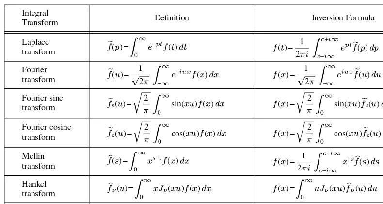
0.5.1.
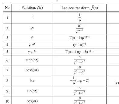
Main Integral Transforms
0.5.2.
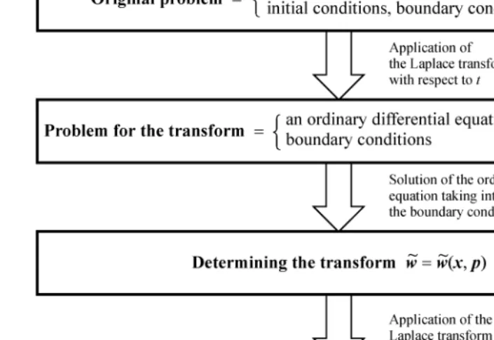
Laplace Transform and Its Application in Mathematical Physics
0.5.3.
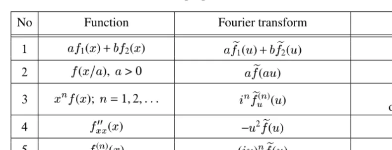
Fourier Transform and Its Application in Mathematical Physics
0.6.
Representation of the Solution of the Cauchy Problem via the Fundamental Solution
0.6.1.
Cauchy Problem for Parabolic Equations
0.6.2.
Cauchy Problem for Hyperbolic Equations
0.7.
Nonhomogeneo
h
us Boundary Value Problems with One Space Variable. Representation
of Solutions via the Green’s Function
0.7.1.
Problems for Parabolic Equations
0.7.2.
Problems for Hyperbolic Equations
0.8.
Nonhomogeneous Boundary Value Problems with Many Space Variables.
Representa-tion of SoluRepresenta-tions via the Green’s FuncRepresenta-tion
0.8.1.
Problems for Parabolic Equations
0.8.2.
Problems for Hyperbolic Equations
0.8.3.
Problems for Elliptic Equations
0.8.4.
Comparison of the Solution Structures for Boundary Value Problems for
Equations of Various Types
0.9.
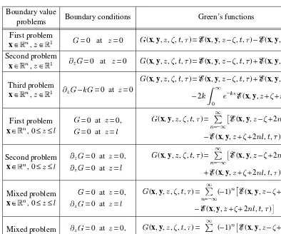
Construction of the Green’s Functions. General Formulas and Relations
0.9.1.
Green’s Functions of Boundary Value Problems for Equations of Various Types
in Bounded Domains
0.10.
Duhamel’s Principles in Nonstationary Problems
0.10.1.
Problems for Homogeneous Linear Equations
0.10.2.
Problems for Nonhomogeneous Linear Equations
0.11.
Transformations Simplifying Initial and Boundary Conditions
0.11.1.
Transformations That Lead to Homogeneous Boundary Conditions
0.11.2.
Transformations That Lead to Homogeneous Initial and Boundary Conditions
1.
Parabolic Equations with One Space Variable
1.1.
Constant Coefficient Equations
1.1.1.
Heat Equation
✖ ❚✖
1.2.
Heat Equation with Axial or Central Symmetry and Related Equations
1.2.1.
Equation of the Form
✖ ❚1.3.
Equations Containing Power Functions and Arbitrary Parameters
1.3.1.
Equations of the Form
✖ ❚✖
1.3.2.
Equations of the Form
✖ ❚✖
1.3.3.
Equations of the Form
✖ ❚✖
1.3.4.
Equations of the Form
✖ ❚✖
1.3.5.
Equations of the Form
✖ ❚✖
1.3.6.
Equations of the Form
✖ ❚✖
1.3.7.
Equations of the Form
✖ ❚✖
1.3.8.
Liquid-Film Mass Transfer Equation
(
1 −
✏2
1.3.9.
Equations of the Form
✤(
✞,
✏)
✖ ❚1.4.
Equations Containing Exponential Functions and Arbitrary Parameters
1.4.1.
Equations of the Form
✖ ❚✖
1.4.2.
Equations of the Form
✖ ❚✖
1.4.3.
Equations of the Form
✖ ❚✖
1.4.4.
Equations of the Form
✖ ❚✖
1.4.5.
Equations of the Form
✖ ❚✖
1.4.6.
Other Equations
1.5.
Equations Containing Hyperbolic Functions and Arbitrary Parameters
1.5.1.
Equations Containing a Hyperbolic Cosine
1.6.
Equations Containing Logarithmic Functions and Arbitrary Parameters
1.6.1.
Equations of the Form
✖ ❚✖
1.6.2.
Equations of the Form
✖ ❚✖
1.7.
Equations Containing Trigonometric Functions and Arbitrary Parameters
1.7.1.
Equations Containing a Cosine
1.7.2.
Equations Containing a Sine
1.7.3.
Equations Containing a Tangent
1.7.4.
Equations Containing a Cotangent
1.8.
Equations Containing Arbitrary Functions
1.8.1.
Equations of the Form
✖ ❚✖
1.8.2.
Equations of the Form
✖ ❚✖
1.8.3.
Equations of the Form
✖ ❚✖
1.8.4.
Equations of the Form
✖ ❚✖
1.8.5.
Equations of the Form
✖ ❚✖
1.8.6.
Equations of the Form
✖ ❚✖
1.8.7.
Equations of the Form
✖ ❚✖
1.8.8.
Equations of the Form
✖ ❚✖
1.9.
Equations of Special Form
1.9.1.
Equations of the Diffusion (Thermal) Boundary Layer
1.9.2.
One-Dimensional Schr ¨odinger Equation
✼❫❪❳✖ ❚
2.
Parabolic Equations with Two Space Variables
2.1.
Heat Equation
✖ ❚2.1.1.
Boundary Value Problems in Cartesian Coordinates
2.1.2.
Problems in Polar Coordinates
2.1.3.
Axisymmetric Problems
2.2.
Heat Equation with a Source
✖ ❚✖
2.2.1.
Problems in Cartesian Coordinates
2.2.2.
Problems in Polar Coordinates
2.2.3.
Axisymmetric Problems
2.3.
Other Equations
2.3.1.
Equations Containing Arbitrary Parameters
2.3.2.
Equations Containing Arbitrary Functions
3.
Parabolic Equations with Three or More Space Variables
3.1.
Heat Equation
✖ ❚3.1.1.
Problems in Cartesian Coordinates
3.1.2.
Problems in Cylindrical Coordinates
3.1.3.
Problems in Spherical Coordinates
3.2.
Heat Equation with Source
✖ ❚✖
3.2.1.
Problems in Cartesian Coordinates
3.2.2.
Problems in Cylindrical Coordinates
3.2.3.
Problems in Spherical Coordinates
3.3.
Other Equations with Three Space Variables
3.4.
Equations with
Space Variables
3.4.1.
Equations of the Form
✖ ❚✖
3.4.2.
Other Equations Containing Arbitrary Parameters
3.4.3.
Equations Containing Arbitrary Functions
4.
Hyperbolic Equations with One Space Variable
4.1.
Constant Coefficient Equations
4.1.1.
Wave Equation
✖2
4.1.2.
Equations of the Form
✖2
4.1.3.
Equation of the Form
✖2
4.1.4.
Equation of the Form
✖2
4.1.5.
Equation of the Form
✖2
4.2.
Wave Equation with Axial or Central Symmetry
4.2.1.
Equations of the Form
✖2
4.2.2.
Equation of the Form
✖2
4.2.3.
Equation of the Form
✖2
4.2.4.
Equation of the Form
✖2
4.2.5.
Equation of the Form
✖2
4.2.6.
Equation of the Form
✖2
4.3.
Equations Containing Power Functions and Arbitrary Parameters
4.3.1.
Equations of the Form
✖2
4.3.2.
Equations of the Form
✖2
4.3.3.
Other Equations
4.4.
Equations Containing the First Time Derivative
4.4.1.
Equations of the Form
✖2
4.4.2.
Equations of the Form
✖2
4.4.3.
Other Equations
4.5.
Equations Containing Arbitrary Functions
4.5.1.
Equations of the Form
❩(
✞)
✖4.5.2.
Equations of the Form
✖2
4.5.3.
Other Equations
5.
Hyperbolic Equations with Two Space Variables
5.1.
Wave Equation
✖2
5.1.1.
Problems in Cartesian Coordinates
5.1.2.
Problems in Polar Coordinates
5.1.3.
Axisymmetric Problems
5.2.
Nonhomogeneous Wave Equation
✖2
5.2.1.
Problems in Cartesian Coordinates
5.2.2.
Problems in Polar Coordinates
5.2.3.
Axisymmetric Problems
5.3.
Equations of the Form
✖2
5.3.1.
Problems in Cartesian Coordinates
5.4.
Telegraph Equation
✖5.4.1.
Problems in Cartesian Coordinates
5.4.2.
Problems in Polar Coordinates
5.4.3.
Axisymmetric Problems
5.5.
Other Equations with Two Space Variables
6.
Hyperbolic Equations with Three or More Space Variables
6.1.
Wave Equation
✖2
6.1.1.
Problems in Cartesian Coordinates
6.1.2.
Problems in Cylindrical Coordinates
6.1.3.
Problems in Spherical Coordinates
6.2.
Nonhomogeneous Wave Equation
✖2
6.2.1.
Problems in Cartesian Coordinates
6.2.2.
Problems in Cylindrical Coordinates
6.2.3.
Problems in Spherical Coordinates
6.3.
Equations of the Form
✖2
6.3.1.
Problems in Cartesian Coordinates
6.3.2.
Problems in Cylindrical Coordinates
6.3.3.
Problems in Spherical Coordinates
6.4.
Telegraph Equation
✖2
6.4.1.
Problems in Cartesian Coordinates
6.4.2.
Problems in Cylindrical Coordinates
6.4.3.
Problems in Spherical Coordinates
6.5.
Other Equations with Three Space Variables
6.5.1.
Equations Containing Arbitrary Parameters
6.5.2.
Equation of the Form
❜(
✞,
✏,
✍)
✖6.6.
Equations with
✆Space Variables
6.6.1.
Wave Equation
✖2
6.6.2.
Nonhomogeneous Wave Equation
✖2
6.6.3.
Equations of the Form
✖2
6.6.4.
Equations Containing the First Time Derivative
7.
Elliptic Equations with Two Space Variables
7.1.
Laplace Equation
✕
2
✓
= 0
7.1.1.
Problems in Cartesian Coordinate System
7.1.2.
Problems in Polar Coordinate System
7.1.3.
Other Coordinate Systems. Conformal Mappings Method
7.2.
Poisson Equation
✕2
✓
= −
❙(x)
7.2.1.
Preliminary Remarks. Solution Structure
7.2.2.
Problems in Cartesian Coordinate System
7.2.3.
Problems in Polar Coordinate System
7.2.4.
Arbitrary Shape Domain. Conformal Mappings Method
7.3.
Helmholtz Equation
✕2
7.3.1.
General Remarks, Results, and Formulas
7.3.2.
Problems in Cartesian Coordinate System
7.3.3.
Problems in Polar Coordinate System
7.4.
Other Equations
7.4.1.
Stationary Schr ¨odinger Equation
✕2
✓
=
✤(
✞,
✏)
✓
7.4.2.
Convective Heat and Mass Transfer Equations
7.4.3.
Equations of Heat and Mass Transfer in Anisotropic Media
7.4.4.
Other Equations Arising in Applications
7.4.5.
Equations of the Form
✦(
✞)
✖8.
Elliptic Equations with Three or More Space Variables
8.1.
Laplace Equation
✕3
✓
= 0
8.1.1.
Problems in Cartesian Coordinates
8.1.2.
Problems in Cylindrical Coordinates
8.1.3.
Problems in Spherical Coordinates
8.1.4.
Other Orthogonal Curvilinear Systems of Coordinates
8.2.
Poisson Equation
✕
3
✓
+
❙(x)
= 0
8.2.1.
Preliminary Remarks. Solution Structure
8.2.2.
Problems in Cartesian Coordinates
8.2.3.
Problems in Cylindrical Coordinates
8.2.4.
Problems in Spherical Coordinates
8.3.
Helmholtz Equation
✕3
8.3.1.
General Remarks, Results, and Formulas
8.3.2.
Problems in Cartesian Coordinates
8.3.3.
Problems in Cylindrical Coordinates
8.3.4.
Problems in Spherical Coordinates
8.3.5.
Other Orthogonal Curvilinear Coordinates
8.4.
Other Equations with Three Space Variables
8.4.1.
Equations Containing Arbitrary Functions
8.4.2.
Equations of the Form div
[
✦(
✞,
✏,
✍)
∇
8.5.
Equations with
✆Space Variables
8.5.1.
Laplace Equation
✕☎
✓
= 0
8.5.2.
Other Equations
9.
Higher-Order Partial Differential Equations
9.1.
Third-Order Partial Differential Equations
9.2.
Fourth-Order One-Dimensional Nonstationary Equations
9.2.1.
Equations of the Form
✖ ❚✖
9.2.2.
Equations of the Form
✖2
9.2.3.
Equations of the Form
✖2
9.2.4.
Equations of the Form
✖2
9.2.5.
Other Equations
9.3.
Two-Dimensional Nonstationary Fourth-Order Equations
9.3.1.
Equations of the Form
✖ ❚✖
9.3.2.
Two-Dimensional Equations of the Form
✖2
-Dimensional Equations of the Form
✖2
9.3.4.
Equations of the Form
✖2
9.3.5.
Equations of the Form
✖2
9.4.
Fourth-Order Stationary Equations
9.4.1.
Biharmonic Equation
✕ ✕
✓
= 0
9.4.2.
Equations of the Form
✕ ✕✓
=
❙9.4.3.
Equations of the Form
✓−
❢✓
=
❙(
✞,
✏)
9.4.4.
Equations of the Form
✖4
❚
✖ ✗
4
+
✖4
❚
✖ ✘
4
=
❙
(
✞,
✏)
9.4.5.
Equations of the Form
✖4
❚
✖ ✗
4
+
✖4
❚
✖ ✘
4
+
✠✓
=
❙(
✞,
✏)
9.4.6.
Stokes Equation (Axisymmetric Flows of Viscous Fluids)
9.5.
Higher-Order Linear Equations with Constant Coefficients
9.5.1.
Fundamental Solutions. Cauchy Problem
9.5.2.
Elliptic Equations
9.5.3.
Hyperbolic Equations
9.5.4.
Regular Equations. Number of Initial Conditions in the Cauchy Problem
9.5.5.
Some Special-Type Equations
9.6.
Higher-Order Linear Equations with Variable Coefficients
9.6.1.
Equations Containing the First Time Derivative
9.6.2.
Equations Containing the Second Time Derivative
9.6.3.
Nonstationary Problems with Many Space Variables
9.6.4.
Some Special-Type Equations
Supplement A. Special Functions and Their Properties
A.1.
Some Symbols and Coefficients
A.1.1.
Factorials
A.1.2.
Binomial Coefficients
A.1.3.
Pochhammer Symbol
A.1.4.
Bernoulli Numbers
A.2.
Error Functions and Exponential Integral
A.2.1.
Error Function and Complementary Error Function
A.2.2.
Exponential Integral
A.2.3.
Logarithmic Integral
A.3.
Sine Integral and Cosine Integral. Fresnel Integrals
A.3.1.
Sine Integral
A.3.2.
Cosine Integral
A.3.3.
Fresnel Integrals
A.4.
Gamma and Beta Functions
A.4.1.
Gamma Function
A.4.2.
Beta Function
A.5.
Incomplete Gamma and Beta Functions
A.5.1.
Incomplete Gamma Function
A.5.2.
Incomplete Beta Function
A.6.
Bessel Functions
A.6.1.
Definitions and Basic Formulas
A.6.2.
Integral Representations and Asymptotic Expansions
A.6.3.
Zeros and Orthogonality Properties of Bessel Functions
A.6.4.
Hankel Functions (Bessel Functions of the Third Kind)
A.7.
Modified Bessel Functions
A.7.1.
Definitions. Basic Formulas
A.7.2.
Integral Representations and Asymptotic Expansions
A.8.
Airy Functions
A.8.1.
Definition and Basic Formulas
A.9.
Degenerate Hypergeometric Functions
A.9.1.
Definitions and Basic Formulas
A.9.2.
Integral Representations and Asymptotic Expansions
A.10.
Hypergeometric Functions
A.10.1.
Definition and Some Formulas
A.10.2.
Basic Properties and Integral Representations
A.11.
Whittaker Functions
A.12.
Legendre Polynomials and Legendre Functions
A.12.1.
Definitions. Basic Formulas
A.12.2.
Zeros of Legendre Polynomials and the Generating Function
A.12.3.
Associated Legendre Functions
A.13.
Parabolic Cylinder Functions
A.13.1.
Definitions. Basic Formulas
A.13.2.
Integral Representations and Asymptotic Expansions
A.14.
Mathieu Functions
A.14.1.
Definitions and Basic Formulas
A.15.
Modified Mathieu Functions
A.16.
Orthogonal Polynomials
A.16.1.
Laguerre Polynomials and Generalized Laguerre Polynomials
A.16.2.
Chebyshev Polynomials and Functions
A.16.3.
Hermite Polynomial
A.16.4.
Jacobi Polynomials
Supplement B. Methods of Generalized and Functional Separation of Variables in
Nonlinear Equations of Mathematical Physics
B.1.
Introduction
B.1.1.
Preliminary Remarks
B.1.2.
Simple Cases of Variable Separation in Nonlinear Equations
B.1.3.
Examples of Nontrivial Variable Separation in Nonlinear Equations
B.2.
Methods of Generalized Separation of Variables
B.2.1.
Structure of Generalized Separable Solutions
B.2.2.
Solution of Functional Differential Equations by Differentiation
B.2.3.
Solution of Functional Differential Equations by Splitting
B.2.4.
Simplified Scheme for Constructing Exact Solutions of Equations with Quadratic
Nonlinearities
B.3.
Methods of Functional Separation of Variables
B.3.1.
Structure of Functional Separable Solutions
B.3.2.
Special Functional Separable Solutions
B.3.3.
Differentiation Method
B.3.4.
Splitting Method. Reduction to a Functional Equation with Two Variables
B.3.5.
Some Functional Equations and Their Solutions. Exact Solutions of Heat and
Wave Equations
B.4.
First-Order Nonlinear Equations
B.4.1.
Preliminary Remarks
B.4.2.
Individual Equations
B.5.
Second-Order Nonlinear Equations
B.5.1.
Parabolic Equations
B.5.2.
Hyperbolic Equations
B.5.3.
Elliptic Equations
B.5.5.
General Form Equations
B.6.
Third-Order Nonlinear Equations
B.6.1.
Stationary Hydrodynamic Boundary Layer Equations
B.6.2.
Nonstationary Hydrodynamic Boundary Layer Equations
B.7.
Fourth-Order Nonlinear Equations
B.7.1.
Stationary Hydrodynamic Equations (Navier–Stokes Equations)
B.7.2.
Nonstationary Hydrodynamic Equations
B.8.
Higher-Order Nonlinear Equations
B.8.1.
Equations of the Form
✖ ❚✖
✬
=
❈ ✲▲✞,
✒
,
✓,
✖ ❚ ✖ ✗,
✡☛✡☛✡,
✖ ❣ ❚ ✖ ✗❣
✳
B.8.2.
Equations of the Form
✖2
❚
✖
✬
2
=
❈
✲▲✞
,
✒
,
✓,
✖ ❚ ✖ ✗,
✡☛✡☛✡,
✖ ❣ ❚ ✖ ✗❣
✳
B.8.3.
Other Equations
Introduction
Some Definitions,
Formulas, Methods, and Solutions
0.1. Classification of Second-Order Partial Differential
Equations
0.1.1. Equations with Two Independent Variables
0.1.1-1. Examples of equations encountered in applications.
Three basic types of partial differential equations are distinguished—
parabolic
,
hyperbolic
, and
elliptic
. The solutions of the equations pertaining to each of the types have their own characteristic
qualitative differences.
The simplest example of a
parabolic
equation is the heat equation
✁
✂
−
2
✁✄
2
= 0
,
(
1
)
where the variables
✂
and
✄
play the role of time and the spatial coordinate, respectively. Note that
equation (1) contains only one highest derivative term.
The simplest example of a
hyperbolic
equation is the wave equation
2
✁✂
2
−
2
✁✄
2
= 0
,
(
2
)
where the variables
✂and
✄play the role of time and the spatial coordinate, respectively. Note that
the highest derivative terms in equation (2) differ in sign.
The simplest example of an
elliptic
equation is the Laplace equation
2
✁✄
2
+
2
✁☎
2
= 0
,
(
3
)
where
✄and
☎play the role of the spatial coordinates. Note that the highest derivative terms in
equation (3) have like signs.
Any linear partial differential equation of the second-order with two independent variables can
be reduced, by appropriate manipulations, to a simpler equation which has one of the three highest
derivative combinations specified above in examples (1), (2), and (3).
0.1.1-2. Types of equations. Characteristic equations.
Consider a second-order partial differential equation with two independent variables which has the
general form
✆
(
✄
,
☎
)
2
✁✄
2
+ 2
✝(
✄
,
☎
)
2
✁ ✄ ☎+
✞(
✄
,
☎
)
2
✁☎
2
=
✟✠
✄
,
☎
,
✁
,
✁
✄
,
✁
where
✆,
✝,
✞are some functions of
and
that have continuous derivatives up to the second-order
inclusive.*
Given a point (
✄,
☎), equation (4) is said to be
parabolic
if
✝2
−
✆✞
= 0
,
hyperbolic
if
✝2
−
✆✞
>
0
,
elliptic
if
✝2
−
✆✞
<
0
at this point.
In order to reduce equation (4) to a canonical form, one should first write out the characteristic
equation
✆ ☛ ☎
2
− 2
✝☛
✄
☛
☎
+
✞☛
✄
2
= 0
,
which splits into two equations
✆ ☛
☎
−
☞✌✝+
✍ ✝2
−
✆✞ ✎
☛
✄
= 0
,
(
5
)
and
✆ ☛
☎
−
☞✌✝−
✍ ✝2
−
✆✞ ✎
☛
✄
= 0
,
(
6
)
and find their general integrals.
0.1.1-3. Canonical form of parabolic equations (case
✝2
−
✆ ✞= 0
).
In this case, equations (5) and (6) coincide and have a common general integral,
✏
(
✄,
☎)
=
✑.
By passing from
✄
,
☎
to new independent variables
✒,
✓in accordance with the relations
✒
=
✏
(
✄,
☎),
✓=
✓(
✄
,
☎),
where
✓=
✓(
✄
,
☎) is any twice differentiable function that satisfies the condition of nondegeneracy
of the Jacobian
✔(
✕,
✖)
✔
(
✗,
✘)
in the given domain, we reduce equation (4) to the canonical form
2
✁✓
2
=
✟1
✠
✒
,
✓,
✁
,
✁
✒
,
✁
✓
✡
.
(
7
)
As
✓, one can take
✓=
✄
or
✓=
☎
.
It is apparent that, just as the heat equation (1), the transformed equation (7) has only one
highest-derivative term.
✙ ✚✜✛ ✢ ✣✥✤ ✦
In the degenerate case where the function
✟1
does not depend on the derivative
✕
✁
,
equation (7) is an ordinary differential equation for the variable
✓, in which
✒serves as a parameter.
0.1.1-4. Canonical form of hyperbolic equations (case
✝2
−
✆ ✞>
0
).
The general integrals
✏
(
✄
,
☎
)
=
✑1
,
✧(
✄
,
☎
)
=
✑2
of equations (5) and (6) are real and different. These integrals determine two different families of
real characteristics.
By passing from
,
to new independent variables
✒,
✓in accordance with the relations
we reduce equation (4) to
2
✁This is the so-called first canonical form of a hyperbolic equation.
The transformation
brings the above equation to another canonical form,
2
✁where
✟3
= 4
✟2
. This is the so-called second canonical form of a hyperbolic equation. Apart from
notation, the left-hand side of the last equation coincides with that of the wave equation (2).
0.1.1-5. Canonical form of elliptic equations (case
✝2
−
✆ ✞<
0
).
In this case the general integrals of equations (5) and (6) are complex conjugate; these determine
two families of complex characteristics.
Let the general integral of equation (5) have the form
✏
) are real-valued functions.
By passing from
✄,
☎to new independent variables
✒,
✓in accordance with the relations
✒
=
we reduce equation (4) to the canonical form
2
✁Apart from notation, the left-hand side of the last equation coincides with that of the Laplace
equation (3).
0.1.2. Equations with Many Independent Variables
Consider a second-order partial differential equation with
✪independent variables
✄
✰
are some functions that have continuous derivatives with respect to all variables to the
second-order inclusive, and
x
= {
✄1
,
✫✬✫✬✫,
✄ ✭
}
. [The right-hand side of equation (8) may be nonlinear.
The left-hand side only is required for the classification of this equation.]
At a point
x
=
x0
, the following quadratic form is assigned to equation (8):
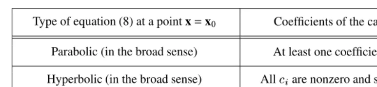
TABLE 1
Classification of equations with many independent variables
Type of equation (8) at a point
x
=
x0
Coefficients of the canonical form (11)
Parabolic (in the broad sense)
At least one coefficient of the
✞✯
is zero
Hyperbolic (in the broad sense)
All
✞✯
are nonzero and some
✞✯
differ in sign
Elliptic
All
✞✯
are nonzero and have like signs
By an appropriate linear nondegenerate transformation
✒
✯
=
✭
✮✳✲
=1
✴✯
✲
✓
✲
(
✩= 1
,
✫✬✫✬✫,
✪)
(
10
)
the quadratic form (9) can be reduced to the canonical form
✱
=
✭
✮
✯
=1
✞
✯
✓
2
✯
,
(
11
)
where the coefficients
✞✯
assume the values
1
,
−1
, and
0
. The number of negative and zero coefficients
in (11) does not depend on the way in which the quadratic form is reduced to the canonical form.
Table 1
presents the basic criteria according to which the equations with many independent
variables are classified.
Suppose all coefficients of the highest derivatives in (8) are constant,
✆✯
✰
=
const. By introducing
the new independent variables
☎
1
,
✫✬✫✬✫,
☎ ✭in accordance with the formulas
☎
✯
=
✭
✵
✲
=1
✴
✯
✲
✄
✲
, where
the
✴
✯
✲
are the coefficients of the linear transformation (10), we reduce equation (8) to the canonical
form
✭✮
✯
=1
✞
✯
2
✁☎
2
✯
=
✟1
✠
y
,
✁
,
✁
☎
1
,
✫✬✫✬✫,
✁
☎ ✭ ✡
.
(
12
)
Here, the coefficients
✞✯
are the same as in the quadratic form (11), and
y
= {
☎1
,
✫✬✫✬✫,
☎ ✭
}
.
✙ ✚✜✛ ✢ ✣✥✤ ✶ ✦
Among the parabolic equations, it is conventional to distinguish the parabolic
equations in the narrow sense, i.e., the equations for which only one of the coefficients,
✞✲
, is zero,
while the other
✞✯
is the same, and in this case the right-hand side of equation (12) must contain the
first-order partial derivative with respect to
☎
✲
.
✙ ✚✜✛ ✢ ✣✥✤ ✷ ✦
In turn, the hyperbolic equations are divided into normal hyperbolic equations—
for which all
✞✯
but one have like signs—and ultrahyperbolic equations—for which there are two or
more positive
✞✯
and two or more negative
✞✯
.
Specific equations of parabolic, elliptic, and hyperbolic types will be discussed further in
Subsection 0.2.
✸✺✹
References for Section
0.1: V. M. Babich, M. B. Kapilevich, S. G. Mikhlin, et al. (1964), S. J. Farlow (1982), D. Colton
(1988), E. Zauderer (1989), A. N. Tikhonov and A. A. Samarskii (1990), I. G. Petrovsky (1991), W. A. Strauss (1992),
R. B. Guenther and J. W. Lee (1996), D. Zwillinger (1998).
0.2. Basic Problems of Mathematical Physics
0.2.1. Initial and Boundary Conditions. Cauchy Problem.
Boundary Value Problems
solutions. The specific solution that describes the physical phenomenon under study is separated
from the set of particular solutions of the given differential equation by means of the initial and
boundary conditions.
Throughout this section, we consider linear equations in the
✪-dimensional Euclidean space
✻
✭
or in an open domain
✼ ✽✻
✭
(exclusive of the boundary) with a sufficiently smooth boundary
✾
=
✼.
0.2.1-1. Parabolic equations. Initial and boundary conditions.
In general, a linear second-order partial differential equation of the parabolic type with
✪independent
variables can be written as
✁✂
−
Parabolic equations govern unsteady thermal, diffusion, and other phenomena dependent on time
✂.
Equation (1) is called homogeneous if
❁(
x
,
✂
)
≡ 0
.
Cauchy problem
(
✂≥ 0
,
x
✽✻
✭
). Find a function
✁that satisfies equation (1) for
✂>
0
and the
Boundary value problem
* (
✂
≥ 0
,
x
✽ ✼). Find a function
✁
that satisfies equation (1) for
✂
>
0
,
the initial condition (3), and the boundary condition
❄
In general,
❄x
,
❀is a first-order linear differential operator in the space variables
x
with coefficient
de-pendent on
x
and
✂. The basic types of boundary conditions are described below in Subsection 0.2.2.
The initial condition (3) is called homogeneous if
❃(
x
)
≡ 0
. The boundary condition (4) is called
homogeneous if
❅(
x
,
✂
)
≡ 0
.
0.2.1-2. Hyperbolic equations. Initial and boundary conditions.
Consider a second-order linear partial differential equation of the hyperbolic type with
✪independent
variables of the general form
2
✁where the linear differential operator
✿x
,
❀is defined by (2). Hyperbolic equations govern unsteady
wave processes, which depend on time
✂.
Equation (5) is said to be homogeneous if
❁(
x
,
✂
)
≡ 0
.
Cauchy problem
(
✂≥ 0
,
x
✽✻
✭
). Find a function
✁that satisfies equation (5) for
✂>
0
and the
initial conditions
✁=
❃0
(
x
)
at
Boundary value problem
(
≥ 0
,
x
✽ ✼). Find a function
that satisfies equation (5) for
>
0
,
the initial conditions (6), and boundary condition (4).
The initial conditions (6) are called homogeneous if
❃0
(
x
)
≡ 0
and
❃1
(
x
)
≡ 0
.
Goursat problem.
On the characteristics of a hyperbolic equation with two independent variables,
the values of the unknown function
✁are prescribed.
0.2.1-3. Elliptic equations. Boundary conditions.
In general, a second-order linear partial differential equation of elliptic type with
✪independent
variables can be written as
−
✿x
[
✁
]
=
❁(
x
),
(
7
)
where
✿
x
[
✁
]
≡
✭
✮
✯
,
✰=1
✆
✯
✰
(
x
)
2
✁✄
✯
✄
✰
+
✭
✮
✯
=1
✝
✯
(
x
)
✁
✄
✯
+
✞(
x
)
✁
,
(
8
)
✭
✮
✯
,
✰=1
✆
✯
✰
(
x
)
✒
✯
✒
✰
≥
❂
✭
✮
✯
=1
✒
2
✯,
❂
>
0
.
Elliptic equations govern steady-state thermal, diffusion, and other phenomena independent of time
✂.
Equation (7) is said to be homogeneous if
❁(
x
)
≡ 0
.
Boundary value problem
. Find a function
✁
that satisfies equation (7) and the boundary condition
❄
x
[
✁
]
=
❅(
x
)
at
x
✽✾
.
(
9
)
In general,
❄x
is a first-order linear differential operator in the space variables
x
. The basic types of
boundary conditions are described below in Subsection 0.2.2.
The boundary condition (9) is called homogeneous if
❅(
x
)
≡ 0
. The boundary value problem
(7)–(9) is said to be homogeneous if
❁≡ 0
and
❅≡ 0
.
0.2.2. First, Second, Third, and Mixed Boundary Value Problems
For any (parabolic, hyperbolic, and elliptic) second-order partial differential equations, it is
con-ventional to distinguish four basic types of boundary value problems, depending on the form of
the boundary conditions (4) [see also the analogous equation (9)]. For simplicity, here we confine
ourselves to the case where the coefficients
✆✯
✰
of equations (1) and (5) have the special form
✆
✯
✰
(
x
,
✂
)
=
✆(
x
,
✂
)
❆✯
✰
,
❆
✯
✰
=
❇
1
if
✩=
❈,
0
if
✩≠
❈.
This situation is rather frequent in applications; such coefficients are used to describe various
phenomena (processes) in isotropic media.
First boundary value problem.
The function
✁(
x
,
✂) takes prescribed values at the boundary
✾of the domain,
✁
(
x
,
✂)
=
❅1
(
x
,
✂
)
for
x
✽✾
.
(
10
)
Second boundary value problem.
The derivative along the (outward) normal is prescribed at the
boundary
✾
of the domain,
✁
❉
=
❅2
(
x
,
✂
)
for
x
✽✾
.
(
11
)
In heat transfer problems, where
✁is temperature, the left-hand side of the boundary condition (11)
is proportional to the heat flux per unit area of the surface
✾Third boundary value problem.
A linear relationship between the unknown function and its
normal derivative is prescribed at the boundary
✾
of the domain,
✁
❉
+
❊(
x
,
✂
)
✁
=
❅3
(
x
,
✂
)
for
x
✽✾
.
(
12
)
Usually, it is assumed that
❊(
x
,
✂
)
=
const. In mass transfer problems, where
✁is concentration, the
boundary condition (12) with
❅3
≡ 0
describes a surface chemical reaction of the first order.
Mixed boundary value problems.
Conditions of various types, listed above, are set at different
portions of the boundary
✾.
If
❅1
≡ 0
,
❅2
≡ 0
, or
❅3
≡ 0
, the respective boundary conditions (10), (11), (12) are said to be
homogeneous.
✸✺✹
References for Section
0.2: V. M. Babich, M. B. Kapilevich, S. G. Mikhlin, et al. (1964), M. A. Pinsky (1984), R. Leis
(1986), R. Haberman (1987), A. A. Dezin (1987), A. G. Mackie (1989), A. N. Tikhonov and A. A. Samarskii (1990),
I. Stakgold (2000).
0.3. Properties and Particular Solutions of Linear
Equations
0.3.1. Homogeneous Linear Equations
0.3.1-1. Preliminary remarks.
For brevity, in this paragraph a homogeneous linear partial differential equation will be written as
❋
[
✁
]
= 0
.
(
1
)
For second-order linear parabolic and hyperbolic equations, the linear differential operator
❋[
✁]
is defined by the left-hand side of equations (1) and (5) from Subsection 0.2.1, respectively. It is
assumed that equation (1) is an arbitrary homogeneous linear partial differential equation of any
order in the variables
✂
,
✄
1
,
✫✬✫✬✫,
✄ ✭with sufficiently smooth coefficients.
A linear operator
❋possesses the properties
❋
[
✁1
+
✁
2
]
=
❋
[
✁1
]
+
❋
[
✁2
],
❋
[
●✁
]
=
●❋
[
✁
],
●=
const.
An arbitrary homogeneous linear equation (1) has a trivial solution,
✁
≡ 0
.
A function
✁
is called a classical solution of equation (1) if
✁
, when substituted into (1), turns
the equation into an identity and if all partial derivatives of
✁
that occur in (1) are continuous; the
notion of a classical solution is directly linked to the range of the independent variables. In what
follows, we usually write “solution” instead of “classical solution” for brevity.
0.3.1-2. Usage of particular solutions for the construction of other particular solutions.
Below are some properties of particular solutions of homogeneous linear equations.
1
❍. Let
✁
1
=
✁
1
(
x
,
✂
),
✁2
=
✁
2
(
x
,
✂
),
✫✬✫✬✫,
✁
✲
=
✁✲
(
x
,
✂) be any particular solutions of the homogeneous
equation (1). Then the linear combination
✁
=
●1
✁
1
+
●2
✁
2
+
■✬■✬■+
●✲
✁
✲
(
2
)
with arbitrary constants
●1
,
●2
,
✫✬✫✬✫,
●✲
is also a solution of equation (1); in physics, this property
is known as the
principle of linear superposition
.
Suppose
{
✁✲
}
is an infinite sequence of solutions of equation (1). Then the series
❏✵
✲
=1
✁
✲
,
irrespective of its convergence, is called a formal solution of (1). If the solutions
✁✲
2
❍. Let the coefficients of the differential operator
❋
be independent of time
. If equation (1) has
a particular solution
❑✁
=
❑✁
(
x
,
✂
), then the partial derivatives of
❑✁
with respect to time,*
❑
are also solutions of equation (1)
3
❍. Let the coefficients of the differential operator
❋
be independent of the space variables
✄
1
,
✫✬✫✬✫,
✄ ✭. If equation (1) has a particular solution
❑✁
=
❑✁
(
x
,
✂), then the partial derivatives of
❑✁
with respect to the space coordinates,
❑
are also solutions of equation (1)
If the coefficients of
❋are independent of only one space coordinate, say
✄
1
, and equation (1)
has a particular solution
❑✁
=
❑✁
(
x
,
✂
), then the partial derivatives
❑
are also solutions of equation (1).
4
❍. Let the coefficients of
❋
be constant and let equation (1) have a particular solution
❑✁
=
❑✁
(
x
,
✂).
Then any particular derivatives of
❑✁
with respect to time and the space coordinates (inclusive mixed
derivatives),
are solutions of equation (1).
5
❍. Suppose equation (1) has a particular solution dependent on a parameter
◆,
❑✁
=
❑✁
(
x
,
✂;
◆), and
the coefficients of
❋are independent of
◆(but can depend on time and the space coordinates). Then,
by differentiating
❑✁
with respect to
◆, one obtains other solutions of equation (1),
❑
belong to the range of the parameter
◆. Then the sum
✁
are arbitrary constants, is also a solution of the homogeneous linear equation (1).
The number of terms in sum (3) can be both finite and infinite.
6
❍. Another effective way of constructing solutions involves the following. The particular solution
❑
✁
(
x
,
✂
;
◆), which depends on the parameter
◆(as before, it is assumed that the coefficients of
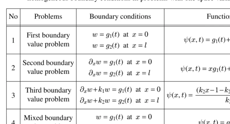
❋
are
independent of
◆), is first multiplied by an arbitrary function
✏
(
◆). Then the resulting expression is
integrated with respect to
◆over some interval [
❖,
✴
]. Thus, one obtains a new function,
P ◗
which is also a solution of the original homogeneous linear equation.
The properties listed in Items
1
❍–
6
❍enable one to use known particular solutions to construct
other particular solutions of homogeneous linear equations of mathematical physics.
* Here and in what follows, it is assumed that the particular solution
❙❚
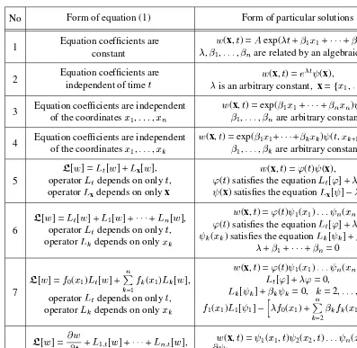
TABLE 2
Homogeneous linear partial differential equations that admit separable solutions
No
Form of equation (1)
Form of particular solutions
1
Equation coefficients are
constant
are related by an algebraic equation
2
Equation coefficients are
independent of time
✂✁
3
Equation coefficients are independent
of the coordinates
✄
are arbitrary constants
4
Equation coefficients are independent
of the coordinates
✄
are arbitrary constants
5
❀
depends on only
✂
,
operator
✿x
depends on only
x
✁
) satisfies the equation
✿ ❀[
❀
depends on only
✂
,
operator
✿✲
depends on only
✄✲
) satisfies the equation
✿ ❀[
) satisfies the equation
✿✲
❀
depends on only
✂
,
operator
✿✲
depends on only
✄
0.3.1-3. Separable solutions.
Many homogeneous linear partial differential equations have solutions that can be represented as the
product of functions depending on different arguments. Such solutions are referred to as separable
solutions.
Table 2
presents the most commonly encountered types of homogeneous linear differential
equa-tions with many independent variables that admit exact separable soluequa-tions. Linear combinaequa-tions of
particular solutions that correspond to different values of the separation parameters,
❨,
✴
1
,
✫✬✫✬✫,
✴
✭