Mastering Machine Learning Spark 2 X 6 pdf pdf

(1)

(2)

Mastering Machine Learning with Spark 2.x

Harness the potential of machine learning, through spark

(3)

Michal Malohlava

(4)

(5)

Mastering Machine Learning with Spark

2.x

transmitted in any form or by any means, without the prior written permission of the publisher, except in the case of brief quotations embedded in critical articles or reviews.

Every effort has been made in the preparation of this book to ensure the accuracy of the information presented. However, the information contained in this book is sold without warranty, either express or implied. Neither the authors, nor Packt Publishing, and its dealers and distributors will be held liable for any damages caused or alleged to be caused directly or indirectly by this book.

Packt Publishing has endeavored to provide trademark information about all of the companies and products mentioned in this book by the appropriate use of capitals. However, Packt Publishing cannot guarantee the accuracy of this information.

First published: August 2017

Production reference: 1290817

Published by Packt Publishing Ltd.

Livery Place

35 Livery Street

Birmingham

B3 2PB, UK.

ISBN 978-1-78528-345-1

(6)

(7)

Credits

Author

Alex Tellez Max Pumperla Michal Malohlava

Copy Editor

Muktikant Garimella

Reviewer

Dipanjan Deb

Project Coordinator

Ulhas Kambali

Commissioning Editor

Veena Pagare

Proofreader

(8)

Acquisition Editor

Larissa Pinto

Indexer

Rekha Nair

Content Development Editor

Nikhil Borkar

Graphics

Jason Monteiro

Technical Editor

Diwakar Shukla

Production Coordinator

(9)

About the Authors

Alex Tellez is a life-long data hacker/enthusiast with a passion for data science and its application to business problems. He has a wealth of experience working across multiple industries, including

banking, health care, online dating, human resources, and online gaming. Alex has also given multiple talks at various AI/machine learning conferences, in addition to lectures at universities about neural networks. When he’s not neck-deep in a textbook, Alex enjoys spending time with family, riding bikes, and utilizing machine learning to feed his French wine curiosity!

First and foremost, I’d like to thank my co-author, Michal, for helping me write this book. As

fellow ML enthusiasts, cyclists, runners, and fathers, we both developed a deeper understanding of each other through this endeavor, which has taken well over one year to create. Simply put, this book would not have been possible without Michal’s support and encouragement.

Next, I’d like to thank my mom, dad, and elder brother, Andres, who have been there every step of the way from day 1 until now. Without question, my elder brother continues to be my hero and is someone that I will forever look up to as being a guiding light. Of course, no acknowledgements would be finished without giving thanks to my beautiful wife, Denise, and daughter, Miya, who have provided the love and support to continue the writing of this book during nights and

weekends. I cannot emphasize enough how much you both mean to me and how you guys are the inspiration and motivation that keeps this engine running. To my daughter, Miya, my hope is that you can pick this book up and one day realize that your old man isn’t quite as silly as I appear to let on.

Last but not least, I’d also like to give thanks to you, the reader, for your interest in this exciting field using this incredible technology. Whether you are a seasoned ML expert, or a newcomer to the field looking to gain a foothold, you have come to the right book and my hope is that you get as much out of this as Michal and I did in writing this work.

Max Pumperla is a data scientist and engineer specializing in deep learning and its applications. He currently works as a deep learning engineer at Skymind and is a co-founder of aetros.com. Max is the author and maintainer of several Python packages, including elephas, a distributed deep learning library using Spark. His open source footprint includes contributions to many popular machine

(10)

Michal Malohlava, creator of Sparkling Water, is a geek and the developer; Java, Linux,

programming languages enthusiast who has been developing software for over 10 years. He obtained his PhD from Charles University in Prague in 2012, and post doctorate from Purdue University.

During his studies, he was interested in the construction of not only distributed but also embedded and real-time, component-based systems, using model-driven methods and domain-specific languages. He participated in the design and development of various systems, including SOFA and Fractal

component systems and the jPapabench control system.

Now, his main interest is big data computation. He participates in the development of the H2O

platform for advanced big data math and computation, and its embedding into Spark engine, published as a project called Sparkling Water.

(11)

About the Reviewer

(12)

Customer Feedback

Thanks for purchasing this Packt book. At Packt, quality is at the heart of our editorial process. To help us improve, please leave us an honest review on this book's Amazon page at https://www.amazon.com /dp/1785283456.

(13)

Preface

Big data – that was our motivation to explore the world of machine learning with Spark a couple of years ago. We wanted to build machine learning applications that would leverag models trained on large amounts of data, but the beginning was not easy. Spark was still evolving, it did not contain a powerful machine learning library, and we were still trying to figure out what it means to build a machine learning application.

But, step by step, we started to explore different corners of the Spark ecosystem and followed Spark’s evolution. For us, the crucial part was a powerful machine learning library, which would provide features such as R or Python libraries did. This was an easy task for us, since we are actively involved in the development of H2O’s machine learning library and its branch called Sparkling

Water, which enables the use of the H2O library from Spark applications. However, model training is just the tip of the machine learning iceberg. We still had to explore how to connect Sparkling Water to Spark RDDs, DataFrames, and DataSets, how to connect Spark to different data sources and read data, or how to export models and reuse them in different applications.

During our journey, Spark evolved as well. Originally, being a pure Scala project, it started to expose Python and, later, R interfaces. It also took its Spark API on a long journey from low-level RDDs to a high-level DataSet, exposing a SQL-like interface. Furthermore, Spark also introduced the concept of machine learning pipelines, adopted from the scikit-learn library known from Python. All these improvements made Spark a great tool for data transformation and data processing.

Based on this experience, we decided to share our knowledge with the rest of the world via this book. Its intention is simple: to demonstrate different aspects of building Spark machine learning applications on examples, and show how to use not only the latest Spark features, but also low-level Spark interfaces. On our journey, we also figure out many tricks and shortcuts not only connected to Spark, but also to the process of developing machine learning applications or source code

organization. And all of them are shared in this book to help keep readers from making the mistakes we made.

The book adopted the Scala language as the main implementation language for our examples. It was a hard decision between using Python and Scala, but at the end Scala won. There were two main

reasons to use Scala: it provides the most mature Spark interface and most applications deployed in production use Scala, mostly because of its performance benefits due to the JVM. Moreover, all source code shown in this book is also available online.

(18)

What this book covers

Chapter 1, Introduction to Large-Scale Machine Learning, invites readers into the land of machine learning and big data, introduces historical paradigms, and describes contemporary tools, including Apache Spark and H2O.

Chapter 2, Detecting Dark Matter: The Higgs-Boson Particle, focuses on the training and evaluation of binomial models.

Chapter 3, Ensemble Methods for Multi-Class Classification, checks into a gym and tries to predict human activities based on data collected from body sensors.

Chapter 4, Predicting Movie Reviews Using NLP, introduces the problem of nature language processing with Spark and demonstrates its power on the sentiment analysis of movie reviews.

Chapter 5, Online Learning with Word2Vec, goes into detail about contemporary NLP techniques.

Chapter 6, Extracting Patterns from Clickstream Data, introduces the basics of frequent pattern mining and three algorithms available in Spark MLlib, before deploying one of these algorithms in a Spark Streaming application.

Chapter 7, Graph Analytics with GraphX, familiarizes the reader with the basic concepts of graphs and graph analytics, explains the core functionality of Spark GraphX, and introduces graph algorithms such as PageRank.

Chapter 8, Lending Club Loan Prediction, combines all the tricks introduced in the previous chapters into end-to-end examples, including data processing, model search and training, and model

(19)

What you need for this book

Code samples provided in this book use Apache Spark 2.1 and its Scala API. Furthermore, we utilize the Sparkling Water package to access the H2O machine learning library. In each chapter, we show how to start Spark using spark-shell, and also how to download the data necessary to run the code.

In summary, the basic requirements to run the code provided in this book include:

(20)

Who this book is for

(21)

Conventions

In this book, you will find a number of text styles that distinguish between different kinds of

information. Here are some examples of these styles and an explanation of their meaning. Code words in text, database table names, folder names, filenames, file extensions, pathnames, dummy URLs, user input, and Twitter handles are shown as follows: "We also appended the magic column row_id, which uniquely identifies each row in the dataset." A block of code is set as follows:

import org.apache.spark.ml.feature.StopWordsRemover

val stopWords= StopWordsRemover.loadDefaultStopWords("english") ++ Array("ax", "arent", "re")

When we wish to draw your attention to a particular part of a code block, the relevant lines or items are set in bold:

val MIN_TOKEN_LENGTH = 3

val toTokens= (minTokenLen: Int, stopWords: Array[String], Any command-line input or output is written as follows:

tar -xvf spark-2.1.1-bin-hadoop2.6.tgz

export SPARK_HOME="$(pwd)/spark-2.1.1-bin-hadoop2.6

New terms and important words are shown in bold. Words that you see on the screen, for example, in menus or dialog boxes, appear in the text like this: "Download the DECLINED LOAN DATA as shown in the following screenshot"

Warnings or important notes appear like this.

(22)

Reader feedback

(23)

Customer support

(24)

Downloading the example code

You can download the example code files for this book from your account at http://www.packtpub.com. If you purchased this book elsewhere, you can visit http://www.packtpub.com/support and register to have the files emailed directly to you. You can download the code files by following these steps:

1. Log in or register to our website using your email address and password. 2. Hover the mouse pointer on the SUPPORT tab at the top.

3. Click on Code Downloads & Errata.

4. Enter the name of the book in the Search box.

5. Select the book for which you're looking to download the code files. 6. Choose from the drop-down menu where you purchased this book from. 7. Click on Code Download.

Once the file is downloaded, please make sure that you unzip or extract the folder using the latest version of:

WinRAR / 7-Zip for Windows Zipeg / iZip / UnRarX for Mac 7-Zip / PeaZip for Linux

(25)

Downloading the color images of this

book

(26)

Errata

(27)

Piracy

(28)

Questions

(29)

Introduction to Large-Scale Machine

Learning and Spark

"Information is the oil of the 21st_{century, and analytics is the combustion engine."}

--Peter Sondergaard, Gartner Research

By 2018, it is estimated that companies will spend $114 billion on big data-related projects, an

increase of roughly 300%, compared to 2013 (https://www.capgemini-consulting.com/resource-file-access/reso urce/pdf/big_data_pov_03-02-15.pdf). Much of this increase in expenditure is due to how much data is being created and how we are better able to store such data by leveraging distributed filesystems such as Hadoop.

However, collecting the data is only half the battle; the other half involves data extraction, transformation, and loading into a computation system, which leverage the power of modern

computers to apply various mathematical methods in order to learn more about data and patterns, and extract useful information to make relevant decisions. The entire data workflow has been boosted in the last few years by not only increasing the computation power and providing easily accessible and scalable cloud services (for example, Amazon AWS, Microsoft Azure, and Heroku) but also by a number of tools and libraries that help to easily manage, control, and scale infrastructure and build applications. Such a growth in the computation power also helps to process larger amounts of data and to apply algorithms that were impossible to apply earlier. Finally, various

computation-expensive statistical or machine learning algorithms have started to help extract nuggets of information from data.

One of the first well-adopted big data technologies was Hadoop, which allows for the

MapReduce computation by saving intermediate results on a disk. However, it still lacks proper big data tools for information extraction. Nevertheless, Hadoop was just the beginning. With the growing size of machine memory, new in-memory computation frameworks appeared, and they also started to provide basic support for conducting data analysis and modeling—for example, SystemML or Spark ML for Spark and FlinkML for Flink. These frameworks represent only the tip of the iceberg—there is a lot more in the big data ecosystem, and it is permanently evolving, since the volume of data is constantly growing, demanding new big data algorithms and processing methods. For example, the

Internet of Things (IoT) represents a new domain that produces huge amount of streaming data from various sources (for example, home security system, Alexa Echo, or vital sensors) and brings not only an unlimited potential to mind useful information from data, but also demands new kind of data

processing and modeling methods.

(30)

Basic working tasks of data scientists

Aspect of big data computation in distributed environment The big data ecosystem

(31)

Data science

Finding a uniform definition of data science, however, is akin to tasting wine and comparing flavor profiles among friends—everyone has their own definition and no one description is more accurate

than the other. At its core, however, data science is the art of asking intelligent questions about data and receiving intelligent answers that matter to key stakeholders. Unfortunately, the opposite also holds true—ask lousy questions of the data and get lousy answers! Therefore, careful formulation of the question is the key for extracting valuable insights from your data. For this reason, companies are now hiring data scientists to help formulate and ask these questions.

(32)

The sexiest role of the 21st century – data

scientist?

At first, it's easy to paint a stereotypical picture of what a typical data scientist looks like: t-shirt, sweatpants, thick-rimmed glasses, and debugging a chunk of code in IntelliJ... you get the idea. Aesthetics aside, what are some of the traits of a data scientist? One of our favorite posters describing this role is shown here in the following diagram:

Figure 2 - What is a data scientist?

(33)

A day in the life of a data scientist

This will probably come as a shock to some of you—being a data scientist is more than reading academic papers, researching new tools, and model building until the wee hours of the morning, fueled on espresso; in fact, this is only a small percentage of the time that a data scientist gets to truly

play (the espresso part however is 100% true for everyone)! Most part of the day, however, is spent in meetings, gaining a better understanding of the business problem(s), crunching the data to learn its limitations (take heart, this book will expose you to a ton of different feature engineering or feature extractions tasks), and how best to present the findings to non data-sciencey people. This is where the true sausage making process takes place, and the best data scientists are the ones who relish in this process because they are gaining more understanding of the requirements and benchmarks for success. In fact, we could literally write a whole new book describing this process from top-to-tail!

So, what (and who) is involved in asking questions about data? Sometimes, it is process of saving data into a relational database and running SQL queries to find insights into data: "for the millions of users that bought this particular product, what are the top 3 OTHER products also bought?" Other times, the question is more complex, such as, "Given the review of a movie, is this a positive or

negative review?" This book is mainly focused on complex questions, like the latter. Answering these types of questions is where businesses really get the most impact from their big data projects and is also where we see a proliferation of emerging technologies that look to make this Q and A system easier, with more functionality.

Some of the most popular, open source frameworks that look to help answer data questions include R, Python, Julia, and Octave, all of which perform reasonably well with small (X < 100 GB) datasets. At this point, it's worth stopping and pointing out a clear distinction between big versus small data. Our general rule of thumb in the office goes as follows:

(34)

Working with big data

What happens when the dataset in question is so vast that it cannot fit into the memory of a single computer and must be distributed across a number of nodes in a large computing cluster? Can't we just rewrite some R code, for example, and extend it to account for more than a single-node

computation? If only things were that simple! There are many reasons why the scaling of algorithms to more machines is difficult. Imagine a simple example of a file containing a list of names:

B D X A D A

We would like to compute the number of occurrences of individual words in the file. If the file fits into a single machine, you can easily compute the number of occurrences by using a combination of the Unix tools, sort and uniq:

bash> sort file | uniq -c

The output is as shown ahead:

2 A 1 B 1 D 1 X

(35)

The machine learning algorithm using a

distributed environment

Machine learning algorithms combine simple tasks into complex patterns, that are even more

complicated in distributed environment. Let's take a simple decision tree algorithm (reference), for example. This particular algorithm creates a binary tree that tries to fit training data and minimize prediction errors. However, in order to do this, it has to decide about the branch of tree it has to send every data point to (don't worry, we'll cover the mechanics of how this algorithm works along with some very useful parameters that you can learn in later in the book). Let's demonstrate it with a simple example:

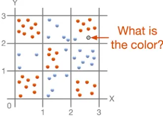
Figure 3 - Example of red and blue data points covering 2D space.

Consider the situation depicted in preceding figure. A two-dimensional board with many points

colored in two colors: red and blue. The goal of the decision tree is to learn and generalize the shape of data and help decide about the color of a new point. In our example, we can easily see that the points almost follow a chessboard pattern. However, the algorithm has to figure out the structure by itself. It starts by finding the best position of a vertical or horizontal line, which would separate the red points from the blue points.

The found decision is stored in the tree root and the steps are recursively applied on both the partitions. The algorithm ends when there is a single point in the partition:

(36)

Splitting of data into multiple machines

For now, let's assume that the number of points is huge and cannot fit into the memory of a single machine. Hence, we need multiple machines, and we have to partition data in such a way that each machine contains only a subset of data. This way, we solve the memory problem; however, it also means that we need to distribute the computation around a cluster of machines. This is the first

difference from single-machine computing. If your data fits into a single machine memory, it is easy to make decisions about data, since the algorithm can access them all at once, but in the case of a

distributed algorithm, this is not true anymore and the algorithm has to be "clever" about accessing the data. Since our goal is to build a decision tree that predicts the color of a new point in the board, we need to figure out how to make the tree that will be the same as a tree built on a single machine.

The naive solution is to build a trivial tree that separates the points based on machine boundaries. But this is obviously a bad solution, since data distribution does not reflect color points at all.

Another solution tries all the possible split decisions in the direction of the X and Y axes and tries to do the best in separating both colors, that is, divides the points into two groups and minimizes the number of points of another color. Imagine that the algorithm is testing the split via the line, X = 1.6. This means that the algorithm has to ask each machine in the cluster to report the result of splitting the machine's local data, merge the results, and decide whether it is the right splitting decision. If it finds an optimal split, it needs to inform all the machines about the decision in order to record which partition each point belongs to.

Compared with the single machine scenario, the distributed algorithm constructing decision tree is more complex and requires a way of distributing the computation among machines. Nowadays, with easy access to a cluster of machines and an increasing demand for the analysis of larger datasets, it becomes a standard requirement.

Even these two simple examples show that for a larger data, proper computation and distributed infrastructure is required, including the following:

A distributed data storage, that is, if the data cannot fit into a single node, we need a way to distribute and process them on multiple machines

A computation paradigm to process and transform the distributed data and to apply mathematical (and statistical) algorithms and workflows

Support to persist and reuse defined workflows and models Support to deploy statistical models in production

In short, we need a framework that will support common data science tasks. It can be considered an unnecessary requirement, since data scientists prefer using existing tools, such as R, Weka, or

(37)

(38)

From Hadoop MapReduce to Spark

With a growing amount of data, the single-machine tools were not able to satisfy the industry needs and thereby created a space for new data processing methods and tools, especially Hadoop

MapReduce, which is based on an idea originally described in the Google paper, MapReduce: Simplified Data Processing on Large Clusters (https://research.google.com/archive/mapreduce.html). On the other hand, it is a generic framework without any explicit support or libraries to create machine learning workflows. Another limitation of classical MapReduce is that it performs many disk I/O operations during the computation instead of benefiting from machine memory.

As you have seen, there are several existing machine learning tools and distributed platforms, but none of them is an exact match for performing machine learning tasks with large data and distributed environment. All these claims open the doors for Apache Spark.

Enter the room, Apache Spark!

Created in 2010 at the UC Berkeley AMP Lab (Algorithms, Machines, People), the Apache Spark project was built with an eye for speed, ease of use, and advanced analytics. One key difference between Spark and other distributed frameworks such as Hadoop is that datasets can be cached in memory, which lends itself nicely to machine learning, given its iterative nature (more on this later!) and how data scientists are constantly accessing the same data many times over.

Spark can be run in a variety of ways, such as the following:

Local mode: This entails a single Java Virtual Machine (JVM) executed on a single host

Standalone Spark cluster: This entails multiple JVMs on multiple hosts

(39)

What is Databricks?

If you know about the Spark project, then chances are high that you have also heard of a company called Databricks. However, you might not know how Databricks and the Spark project are related to one another. In short, Databricks was founded by the creators of the Apache Spark project and accounts for over 75% of the code base for the Spark project. Aside from being a huge force behind the Spark project with respect to development, Databricks also offers various certifications in Spark for developers, administrators, trainers, and analysts alike. However, Databricks is not the only main contributor to the code base; companies such as IBM, Cloudera, and Microsoft also actively

participate in Apache Spark development.

As a side note, Databricks also organizes the Spark Summit (in both Europe and the US), which is the premier Spark conference and a great place to learn about the latest developments in the project and how others are using Spark within their ecosystem.

Throughout this book, we will give recommended links that we read daily that offer great insights and also important changes with respect to the new versions of Spark. One of the best resources here is the Databricks blog, which is constantly being updated with great content. Be sure to regularly check this out at https://databricks.com/blog.

(40)

Inside the box

So, you have downloaded the latest version of Spark (depending on how you plan on launching Spark) and you have run the standard Hello, World! example....what now?!

Spark comes equipped with five libraries, which can be used separately--or in unison--depending on the task we are trying to solve. Note that in this book, we plan on using a variety of different libraries, all within the same application so that you will have the maximum exposure to the Spark platform and better understand the benefits (and limitations) of each library. These five libraries are as follows:

Core: This is the Spark core infrastructure, providing primitives to represent and store data called Resilient Distributed Dataset (RDDs) and manipulate data with tasks and jobs.

SQL : This library provides user-friendly API over core RDDs by introducing DataFrames and SQL to manipulate with the data stored.

MLlib (Machine Learning Library) : This is Spark's very own machine learning library of algorithms developed in-house that can be used within your Spark application.

Graphx : This is used for graphs and graph-calculations; we will explore this particular library in depth in a later chapter.

Streaming : This library allows real-time streaming of data from various sources, such as

Kafka, Twitter, Flume, and TCP sockets, to name a few. Many of the applications we will build in this book will leverage the MLlib and Streaming libraries to build our applications.

(41)

Introducing H2O.ai

H2O is an open source, machine learning platform that plays extremely well with Spark; in fact, it was one of the first third-party packages deemed "Certified on Spark".

Sparkling Water (H2O + Spark) is H2O's integration of their platform within the Spark project, which combines the machine learning capabilities of H2O with all the functionality of Spark. This means that users can run H2O algorithms on Spark RDD/DataFrame for both exploration and deployment purposes. This is made possible because H2O and Spark share the same JVM, which allows for seamless transitions between the two platforms. H2O stores data in the H2O frame, which is a columnar-compressed representation of your dataset that can be created from Spark RDD and/or DataFrame. Throughout much of this book, we will be referencing algorithms from Spark's MLlib library and H2O's platform, showing how to use both the libraries to get the best results possible for a given task.

The following is a summary of the features Sparkling Water comes equipped with:

Use of H2O algorithms within a Spark workflow

Transformations between Spark and H2O data structures

Use of Spark RDD and/or DataFrame as inputs to H2O algorithms

Use of H2O frames as inputs into MLlib algorithms (will come in handy when we do feature engineering later)

Transparent execution of Sparkling Water applications on top of Spark (for example, we can run a Sparkling Water application within a Spark stream)

(42)

Design of Sparkling Water

Sparkling Water is designed to be executed as a regular Spark application. Consequently, it is launched inside a Spark executor created after submitting the application. At this point, H2O starts services, including a distributed key-value (K/V) store and memory manager, and orchestrates them into a cloud. The topology of the created cloud follows the topology of the underlying Spark cluster.

As stated previously, Sparkling Water enables transformation between different types of

RDDs/DataFrames and H2O's frame, and vice versa. When converting from a hex frame to an RDD, a wrapper is created around the hex frame to provide an RDD-like API. In this case, data is not

duplicated but served directly from the underlying hex frame. Converting from an RDD/DataFrame to a H2O frame requires data duplication because it transforms data from Spark into H2O-specific storage. However, data stored in an H2O frame is heavily compressed and does not need to be preserved as an RDD anymore:

(43)

What's the difference between H2O and

Spark's MLlib?

As stated previously, MLlib is a library of popular machine learning algorithms built using Spark. Not surprisingly, H2O and MLlib share many of the same algorithms but differ in both their

(44)

One other nice addition is that H2O allows data scientists to grid search many hyper-parameters that ship with their algorithms. Grid search is a way of optimizing all the hyperparameters of an algorithm to make model configuration easier. Often, it is difficult to know which hyperparameters to change and how to change them; the grid search allows us to explore many hyperparameters simultaneously, measure the output, and help select the best models based on our quality requirements. The H2O grid search can be combined with model cross-validation and various stopping criteria, resulting in

(45)

Data munging

(46)

Data science - an iterative process

Often, the process flow of many big data projects is iterative, which means a lot of back-and-forth testing new ideas, new features to include, tweaking various hyper-parameters, and so on, with a fail fast attitude. The end result of these projects is usually a model that can answer a question being posed. Notice that we didn't say accurately answer a question being posed! One pitfall of many data scientists these days is their inability to generalize a model for new data, meaning that they have

overfit their data so that the model provides poor results when given new data. Accuracy is extremely task-dependent and is usually dictated by the business needs with some sensitivity analysis being done to weigh the cost-benefits of the model outcomes. However, there are a few standard accuracy measures that we will go over throughout this book so that you can compare various models to see

how changes to the model impact the result.

H2O is constantly giving meetup talks and inviting others to give machine learning meetups around the US and Europe. Each meetup or conference slides is available on SlideShare (http://www.slideshare.com/0xdata) or YouTube. Both the sites serve as great

sources of information not only about machine learning and statistics but also about distributed systems and computation. For example, one of the most interesting

(47)

Summary

In this chapter, we wanted to give you a brief glimpse into the life of a data scientist, what this entails, and some of the challenges that data scientists consistently face. In light of these challenges, we feel that the Apache Spark project is ideally positioned to help tackle these topics, which range from data ingestion and feature extraction/creation to model building and deployment. We

intentionally kept this chapter short and light on verbiage because we feel working through examples and different use cases is a better use of time as opposed to speaking abstractly and at length about a given data science topic. Throughout the rest of this book, we will focus solely on this process while giving best-practice tips and recommended reading along the way for users who wish to learn more. Remember that before embarking on your next data science project, be sure to clearly define the problem beforehand, so you can ask an intelligent question of your data and (hopefully) get an intelligent answer!

(48)

Detecting Dark Matter - The Higgs-Boson

Particle

True or false? Positive or negative? Pass or no pass? User clicks on the ad versus not clicking the ad? If you've ever asked/encountered these questions before then you are already familiar with the

concept of binary classification.

At it's core, binary classification - also referred to as binomial classification - attempts to categorize a set of elements into two distinct groups using a classification rule, which in our case, can be a

machine learning algorithm. This chapter shows how to deal with it in the context of Spark and big data. We are going to explain and demonstrate:

Spark MLlib models for binary classification including decision trees, random forest, and the gradient boosted machine

Binary classification support in H2O

(49)

Type I versus type II error

Binary classifiers have intuitive interpretation since they are trying to separate data points into two groups. This sounds simple, but we need to have some notion of measuring the quality of this

separation. Furthermore, one important characteristic of a binary classification problem is that, often, the proportion of one group of labels versus the other can be disproportionate. That means the dataset may be imbalanced with respect to one label which necessitates careful interpretation by the data scientist.

Suppose, for example, we are trying to detect the presence of a particular rare disease in a population of 15 million people and we discover that - using a large subset of the population - only 10,000 or 10 million individuals actually carry the disease. Without taking this huge disproportion into

consideration, the most naive algorithm would guess "no presence of disease" on the remaining five million people simply because 0.1% of the subset carried the disease. Suppose that of the remaining five million people, the same proportion, 0.1%, carried the disease, then these 5,000 people would not be correctly diagnosed because the naive algorithm would simply guess no one carries the

disease. Is this acceptable? In this situation, the cost of the errors posed by binary classification is an important factor to consider, which is relative to the question being asked.

Given that we are only dealing with two outcomes for this type of problem, we can create a 2-D representation of the different types of errors that are possible. Keeping our preceding example of the people carrying / not carrying the disease, we can think about the outcome of our classification rule as follows:

Figure 1 - Relation between predicted and actual values

From the preceding table, the green area represents where we are correctly predicting the presence / absence of disease in the individual whereas the white areas represent where our prediction was incorrect. These false predictions fall into two categories known as Type I and Type II errors:

Type I error: When we reject the null hypothesis (that is, a person not carrying the disease) when in fact, it is true in actuality

(50)

Clearly, both errors are not good but often, in practice, some errors are more acceptable than others.

(51)

Finding the Higgs-Boson particle

On July 4, 2012, scientists from Europe's CERN lab in Geneva, Switzerland, presented strong evidence of a particle they believe is the Higgs-Boson, sometimes referred to as the God-particle. Why is this discovery so meaningful and important? As popular physicist and author Michio Kaku wrote:

"In quantum physics, it was a Higgs-like particle that sparked the cosmic explosion (that is, the big bang). In other words, everything we see around us, including galaxies, stars, planets, and us, owes its existence to the Higgs-Boson."

(52)

The LHC and data creation

To test for the presence of the Higgs-Boson, scientists constructed the largest human-made machine called the Large Hadron Collider (LHC) near Geneva, close to the Franco-Swiss border. The LHC is a ring-shaped tunnel that runs 27 kilometers long (equivalent to the Circle Line from London's Underground) and lies 100 meters underground.

Through this tunnel, subatomic particles are fired in opposite directions with the help of the

(53)

The theory behind the Higgs-Boson

For quite some time, physicists have known that some fundamental particles have mass which contradicts the mathematics underlying the Standard Model which states these particles should be mass-less. In the 1960s, Peter Higgs and his colleagues challenged this mass conundrum by studying the universe after the big bang. At the time, it was largely believed that particles should be thought of as ripples in a quantum jelly as opposed to tiny billiard balls bouncing off one another. Higgs

believed that during this early period, all particle jellies were runny with a consistency like water; but as the universe began to cool down, one particle jelly, known first as the Higgs field, began to condense and become thick. Consequently, other particle jellies, when interacting with the Higgs field, are drawn towards it thanks to inertia; and, according to Sir Isaac Newton, any particle with inertia should contain mass. This mechanism offers an explanation to how particles that makeup the Standard Model - born massless at first - may have acquired mass. It follows then that the amount of mass acquired by each particle is proportional to the strength with which it feels the effects of the Higgs field.

The article https://plus.maths.org/content/particle-hunting-lhc-higgs-boson is a great source

(54)

Measuring for the Higgs-Boson

Testing this theory goes back to the original notion of particle jelly ripples and in particular, the Higgs jelly which a) can ripple and b) would resemble a particle in an experiment: the infamous Higgs-Boson. So how do scientists detect this ripple using the LHC?

(55)

The dataset

Upon releasing their findings to the scientific community in 2012, researchers later made the data public from the LHC experiments where they observed - and identified - a signal which is indicative of the Higgs-Boson particle. However, amidst the positive findings is a lot of background noise

which causes an imbalance within the dataset. Our task as data scientist is to build a machine learning model which can accurately identify the Higgs-Boson particle from background noise. Already, you should be thinking about how this question is phrased which would be indicative of binary

classification (that is, is this example the Higgs-Boson versus background noise?).

You can download the dataset from https://archive.ics.uci.edu/ml/datasets/HIGGS or use the

script getdata.sh located in the bin folder of this chapter.

This file is 2.6 gigs (uncompressed) and contains 11 million examples that have been labeled as 0 -background noise and 1 - Higgs-Boson. First, you will need to uncompress this file and then we will begin loading the data into Spark for processing and analysis. There are 29 total fields which make up the dataset:

Field 1: Class label (1 = signal for Higgs-Boson, 2 = background noise) Fields 2-22: 21 "low-level" features that come from the collision detectors

Fields 23-29: seven "high-level" features that have been hand-derived by particle physicists to help classify the particle into its appropriate class (Higgs or background noise)

Later in this chapter, we cover a Deep Neural Network (DNN) example that will attempt to

learn these hand-derived features through layers of non-linear transformations to the input data.

(56)

Spark start and data load

Now it's time to fire up a Spark cluster which will give us all the functionality of Spark while simultaneously allowing us to use H2O algorithms and visualize our data. As always, we must download Spark 2.1 distribution from http://spark.apache.org/downloads.html and declare the execution environment beforehand. For example, if you download spark-2.1.1-bin-hadoop2.6.tgz from the Spark download page, you can prepare the environment in the following way:

tar -xvf spark-2.1.1-bin-hadoop2.6.tgz

export SPARK_HOME="$(pwd)/spark-2.1.1-bin-hadoop2.6

When the environment is ready, we can start the interactive Spark shell with Sparkling Water packages and this book package:

H2O.ai is constantly keeping up with the latest releases of the Spark project to match the version of Sparkling Water. The book is using Spark 2.1.1 distribution and

Sparkling Water 2.1.12. You can find the latest version of Sparkling Water for your version of Spark at http://h2o.ai/download/

This case is using the provided Spark shell which downloads and uses Spark

packages of Sparkling Water version 2.1.12. The packages are identified by Maven coordinates - in this case ai.h2o represents organization ID, sparkling-water-core

identifies Sparkling Water implementation (for Scala 2.11, since Scala versions are not binary compatible), and, finally, 2.1.12 is a version of the package. Furthermore, we are using this book -specific package which provides handful utilities.

The list of all published Sparkling Water versions is also available on Maven central: http://search.maven.org

(57)

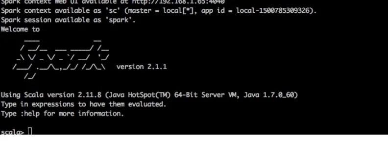
Figure 2 - Notice how the shell starts up showing you the version of Spark you are using.

The provided book source code provides for each chapter the command starting the Spark environment; for this chapter, you can find it in the chapter2/bin folder.

The Spark shell is a Scala - based console application that accepts Scala code and executes it in an interactive way. The next step is to prepare the computation environment by importing packages which we are going to use during our example.

import org.apache.spark.mllib

Let's first ingest the .csv file that you should have downloaded and do a quick count to see how much data is in our subset. Here, please notice, that the code expects the data folder "data" relative to the current process working directory or location specified:

val rawData = sc.textFile(s"${sys.env.get("DATADIR").getOrElse("data")}/higgs100k.csv") println(s"Number of rows: ${rawData.count}")

The output is as follows:

You can observe that execution of the command sc.textFile(...) took no time and returned instantly, while executing rawData.count took the majority amount of time. This exactly demonstrates the

(58)

independent.

Right now, we defined a transformation which loads data into the Spark data structure RDD[String] which contains all the lines of input data file. So, let's look at the first two rows:

rawData.take(2)

The first two lines contain raw data as loaded from the file. You can see that a row is composed of a response column having the value 0,1 (the first value of the row) and other columns having real

values. However, the lines are still represented as strings and require parsing and transformation into regular rows. Hence, based on the knowledge of the input data format, we can define a simple parser which splits an input line into numbers based on a comma:

val data = rawData.map(line => line.split(',').map(_.toDouble))

Now we can extract a response column (the first column in the dataset) and the rest of data representing the input features:

val response: RDD[Int] = data.map(row => row(0).toInt)

val features: RDD[Vector] = data.map(line => Vectors.dense(line.slice(1, line.size)))

After this transformation, we have two RDDs:

One representing the response column

Another which contains dense vectors of numbers holding individual input features

Next, let's look in more detail at the input features and perform some very rudimentary data analysis:

val featuresMatrix = new RowMatrix(features)

val featuresSummary = featuresMatrix.computeColumnSummaryStatistics()

We converted this vector into a distributed RowMatrix. This gives us the ability to perform simple summary statistics (for example, compute mean, variance, and so on:)

import org.apache.spark.utils.Tabulizer._

(59)

Take a look at following code:

println(s"Higgs Features Variance Values = ${table(featuresSummary.variance, 8)}")

In the next step, let's explore columns in more details. We can get directly the number of non-zeros in each column to figure out if the data is dense or sparse. Dense data contains mostly non-zeros, sparse data the opposite. The ratio between the number of non-zeros in the data and the number of all values represents the sparsity of data. The sparsity can drive our selection of the computation method, since for sparse data it is more efficient to iterate over non-zeros only:

val nonZeros = featuresSummary.numNonzeros

println(s"Non-zero values count per column: ${table(nonZeros, cols = 8, format = "%.0f")}")

However, the call just gives us the number of non-zeros for all column, which is not so interesting. We are more curious about columns that contain some zero values:

val numRows = featuresMatrix.numRows val numCols = featuresMatrix.numCols val colsWithZeros = nonZeros

.toArray .zipWithIndex

.filter { case (rows, idx) => rows != numRows }

println(s"Columns with zeros:\n${table(Seq("#zeros", "column"), colsWithZeros, Map.empty[Int, String])}")

(60)

We can see that columns 8, 12, 16, and 20 contain some zero numbers, but still not enough to consider the matrix as sparse. To confirm our observation, we can compute the overall sparsity of the matrix (remainder: the matrix does not include the response column):

val sparsity = nonZeros.toArray.sum / (numRows * numCols) println(f"Data sparsity: ${sparsity}%.2f")

And the computed number confirms our former observation - the input matrix is dense.

Now it is time to explore the response column in more detail. As the first step, we verify that the response contains only the values 0 and 1 by computing the unique values inside the response vector:

val responseValues = response.distinct.collect

println(s"Response values: ${responseValues.mkString(", ")}")

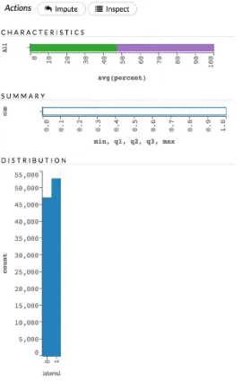
The next step is to explore the distribution of labels in the response vector. We can compute the rate directly via Spark:

val responseDistribution = response.map(v => (v,1)).countByKey println(s"Response distribution:\n${table(responseDistribution)}")

In this step, we simply transform each row into a tuple representing the row value and 1 expressing that the value occurs once in the row. Having RDDs of pairs, the Spark method countByKey aggregates pairs by a key and gives us a summary of the keys count. It shows that the data surprisingly contains slightly more cases which do represent Higgs-Boson but we can still consider the response nicely balanced.

(61)

start H2O services represented by H2OContext:

import org.apache.spark.h2o._

val h2oContext = H2OContext.getOrCreate(sc)

The code initializes the H2O library and starts H2O services on each node of the Spark clusters. It also exposes an interactive environment called Flow, which is useful for data exploration and model building. In the console, h2oContext prints the location of the exposed UI:

h2oContext: org.apache.spark.h2o.H2OContext =

Open H2O Flow in browser: http://192.168.1.65:54321 (CMD + click in Mac OSX)

Now we can directly open the Flow UI address and start exploring the data. However, before doing that, we need to publish the Spark data as an H2O frame called response:

val h2oResponse = h2oContext.asH2OFrame(response, "response")

If you import implicit conversions exposed by H2OContext, you will be able to invoke transformation transparently based on the defined type on the left-side of

assignment:

For example:

import h2oContext.implicits._

val h2oResponse: H2OFrame = response

(62)

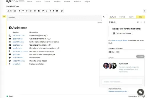
Figure 3 - Interactive Flow UI

The Flow UI allows for interactive work with the stored data. Let,s look at which data is exposed for the Flow by typing getFrames into the highlighted cell:

Figure 4 - Get list of available H2O frames

(63)

(64)

Labeled point vector

Prior to running any supervised machine learning algorithm using Spark MLlib, we must convert our dataset into a labeled point vector which maps features to a given label/response; labels are stored as doubles which facilitates their use for both classification and regression tasks. For all binary

classification problems, labels should be stored as either 0 or 1, which we confirmed from the preceding summary statistics holds true for our example.

val higgs = response.zip(features).map { case (response, features) =>

LabeledPoint(response, features) } higgs.setName("higgs").cache()

An example of a labeled point vector follows:

(1.0, [0.123, 0.456, 0.567, 0.678, ..., 0.789])

In the preceding example, all doubles inside the bracket are the features and the single number outside the bracket is our label. Note that we are yet to tell Spark that we are performing a classification task and not a regression task which will happen later.

In this example, all input features contain only numeric values, but in many

(65)

Data caching

Many machine learning algorithms are iterative in nature and thus require multiple passes over the data. However, all data stored in Spark RDD are by default transient, since RDD just stores the transformation to be executed and not the actual data. That means each action would recompute data again and again by executing the transformation stored in RDD.

Hence, Spark provides a way to persist the data in case we need to iterate over it. Spark also publishes several StorageLevels to allow storing data with various options:

NONE: No caching at all

MEMORY_ONLY: Caches RDD data only in memory

DISK_ONLY: Write cached RDD data to a disk and releases from memory

MEMORY_AND_DISK: Caches RDD in memory, if it's not possible to offload data to a disk OFF_HEAP: Use external memory storage which is not part of JVM heap

Furthermore, Spark gives users the ability to cache data in two flavors: raw (for example, MEMORY_ONLY) and serialized (for example, MEMORY_ONLY_SER). The later uses large memory buffers to store serialized content of RDD directly. Which one to use is very task and resource dependent. A good rule of thumb is if the dataset you are working with is less than 10 gigs then raw caching is preferred to serialized caching. However, once you cross over the 10 gigs soft-threshold, raw caching imposes a greater memory footprint than serialized caching.

Spark can be forced to cache by calling the cache() method on RDD or directly via calling the method persist with the desired persistent target - persist(StorageLevels.MEMORY_ONLY_SER). It is useful to know that RDD allows us to set up the storage level only once.

The decision on what to cache and how to cache is part of the Spark magic; however, the golden rule is to use caching when we need to access RDD data several times and choose a destination based on the application preference respecting speed and storage. A great blogpost which goes into far more detail than what is given here is available at:

http://sujee.net/2015/01/22/understanding-spark-caching/#.VpU1nJMrLdc

(66)

Creating a training and testing set

As with most supervised learning tasks, we will create a split in our dataset so that we teach a model on one subset and then test its ability to generalize on new data against the holdout set. For the

purposes of this example, we split the data 80/20 but there is no hard rule on what the ratio for a split should be - or for that matter - how many splits there should be in the first place:

// Create Train & Test Splits

val trainTestSplits = higgs.randomSplit(Array(0.8, 0.2))

val (trainingData, testData) = (trainTestSplits(0), trainTestSplits(1))

By creating our 80/20 split on the dataset, we are taking a random sample of 8.8 million examples as our training set and the remaining 2.2 million as our testing set. We could just as easily take another random 80/20 split and generate a new training set with the same number of examples (8.8 million) but with different data. Doing this type of hard splitting of our original dataset introduces a sampling bias, which basically means that our model will learn to fit the training data but the training data may not be representative of "reality". Given that we are working with 11 million examples already, this bias is not as prominent versus if our original dataset is 100 rows, for example. This is often referred to as the holdout method for model validation.

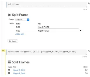
You can also use the H2O Flow to split the data:

1. Publish the Higgs data as H2OFrame:

val higgsHF = h2oContext.asH2OFrame(higgs.toDF, "higgsHF")

2. Split data in the Flow UI using the command splitFrame (see Figure 07). 3. And then publish the results back to RDD.

(67)

In contrast to Spark lazy evaluation, the H2O computation model is eager. That means the splitFrame invocation processes the data right away and creates two new frames, which can be directly

(68)

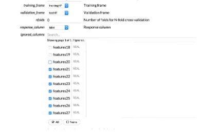
What about cross-validation?

Often, in the case of smaller datasets, data scientists employ a technique known as cross-validation, which is also available to you in Spark. The CrossValidator class starts by splitting the dataset into N-folds (user declared) - each fold is used N-1 times as part of the training set and once for model

validation. For example, if we declare that we wish to use a 5-fold cross-validation, the CrossValidator class will create five pairs (training and testing) of datasets using four-fifths of the dataset to create the training set with the final fifth as the test set, as shown in the following figure.

The idea is that we would see the performance of our algorithm across different, randomly sampled datasets to account for the inherent sampling bias when we create our training/testing split on 80% of the data. An example of a model that does not generalize well would be one where the accuracy - as measured by overall error, for example - would be all over the map with wildly different error rates, which would suggest we need to rethink our model.

Figure 8 - Conceptual schema of 5-fold cross-validation.

There is no set rule on how many folds you should perform, as these questions are highly individual with respect to the type of data being used, the number of examples, and so on. In some cases, it makes sense to have extreme cross-validation where N is equal to the number of data points in the input dataset. In this case, the Test set contains only one row. This method is called as Leave-One-Out (LOO) validation and is more computationally expensive.

(69)

Our first model – decision tree

Our first attempt at trying to classify the Higgs-Boson from background noise will use a decision tree algorithm. We purposely eschew from explaining the intuition behind this algorithm as this has

already been well documented with plenty of supporting literature for the reader to consume (http://ww w.saedsayad.com/decision_tree.htm, http://spark.apache.org/docs/latest/mllib-decision-tree.html). Instead, we will focus on the hyper-parameters and how to interpret the model's efficacy with respect to certain criteria / error measures. Let's start with the basic parameters:

val numClasses = 2

val categoricalFeaturesInfo = Map[Int, Int]() val impurity = "gini"

val maxDepth = 5 val maxBins = 10

Now we are explicitly telling Spark that we wish to build a decision tree classifier that looks to distinguish between two classes. Let's take a closer look at some of the hyper-parameters for our decision tree and see what they mean:

numClasses: How many classes are we trying to classify? In this example, we wish to distinguish between the Higgs-Boson particle and background noise and thus there are four classes:

categoricalFeaturesInfo: A specification whereby we declare what features are categorical features and should not be treated as numbers (for example, ZIP code is a popular example). There are no categorical features in this dataset that we need to worry about.

impurity: A measure of the homogeneity of the labels at the node. Currently in Spark, there are two measures of impurity with respect to classification: Gini and Entropy and one impurity for regression: variance.

maxDepth: A stopping criterion which limits the depth of constructed trees. Generally, deeper trees lead to more accurate results but run the risk of overfitting.

maxBins: Number of bins (think "values") for the tree to consider when making splits. Generally, increasing the number of bins allows the tree to consider more values but also increases

(70)

Gini versus Entropy

In order to determine which one of the impurity measures to use, it's important that we cover some foundational knowledge beginning with the concept of information gain.

At it's core, information gain is as it sounds: the gain in information from moving between two states. More accurately, the information gain of a certain event is the difference between the amount of

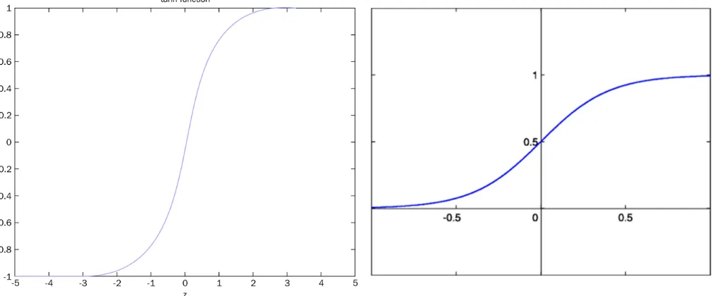
information known before and after the event takes place. One common measure of this information is looking at the Entropy which can be defined as:

Where p_j is the frequency of label j at a node.

Now that you are familiar with the concept of information gain and Entropy, we can move on to what is meant by the Gini Index (there is no correlation whatsoever to the Gini coefficient).

The Gini Index: is a measure of how often a randomly chosen element would be misclassified if it were randomly given a label according to the distribution of labels at a given node.

Compared with the equation for Entropy, the Gini Index should be computed slightly faster due to the absence of a log computation which may be why it is the default option for many other machine learning libraries including MLlib.

But does this make it a better measure for which to make splits for our decision tree? It turns out that the choice of impurity measure has little effect on performance with respect to single decision tree algorithms. The reason for this, according to Tan et. al, in the book Introduction to Data Mining, is that:

"...This is because impurity measures are quite consistent with each other [...]. Indeed, the

strategy used to prune the tree has a greater impact on the final tree than the choice of impurity measure."

Now it's time we train our decision tree classifier on the training data:

(71)

println("Decision Tree Model:\n" + dtreeModel.toDebugString)

This should yield a final output which looks like this (note that your results will be slightly different due to the random split of the data):

The output shows that decision tree has depth 5 and 63 nodes organized in an hierarchical decision predicate. Let's go ahead and interpret it looking at the first five decisions. The way it reads is: "If feature 25's value is less than or equal to 1.0559 AND is less than or equal to 0.61558 AND feature 27's value is less than or equal to 0.87310 AND feature 5's value is less than or equal to 0.89683 AND finally, feature 22's value is less than or equal to 0.76688, then the prediction is 1.0 (the Higgs-Boson). BUT, these five conditions must be met in order for the prediction to hold."

Notice that if the last condition is not held (feature 22's value is > 0.76688) but the previous four held conditions remain true, then the prediction changes from 1 to 0, indicating background noise.

Now, let's score the model on our test dataset and print the prediction error:

val treeLabelAndPreds = testData.map { point =>

val prediction = dtreeModel.predict(point.features) (point.label.toInt, prediction.toInt)

}

val treeTestErr = treeLabelAndPreds.filter(r => r._1 != r._2).count.toDouble / testData.count() println(f"Tree Model: Test Error = ${treeTestErr}%.3f")

(72)

which we defined in the preceding code. Again, your error rate will be slightly different than ours but as we show, our simple decision tree model has an error rate of ~33%. However, as you know, there are different kinds of errors that we can possibly make and so it's worth exploring what those types of error are by constructing a confusion matrix:

val cm = treeLabelAndPreds.combineByKey(

createCombiner = (label: Int) => if (label == 0) (1,0) else (0,1),

mergeValue = (v:(Int,Int), label:Int) => if (label == 0) (v._1 +1, v._2) else (v._1, v._2 + 1), mergeCombiners = (v1:(Int,Int), v2:(Int,Int)) => (v1._1 + v2._1, v1._2 + v2._2)).collect

The preceding code is using advanced the Spark method combineByKey which allows us to map each (K,V)-pair to a value, which is going to represent the output of the group by the key operation. In this case, the (K,V)-pair represents the actual value K and prediction V. We map each prediction to a tuple by creating a combiner (parameter createCombiner) - if the predicted values is 0, then we map to (1,0); otherwise, we map to (0,1). Then we need to define how combiners accept a new value and how combiners are merged together. At the end, the method produces:

cm: Array[(Int, (Int, Int))] = Array((0,(5402,4131)), (1,(2724,7846)))

The resulting array contains two tuples - one for the actual value 0 and another for the actual value 1. Each tuple contains the number of predictions 0 and 1. Hence, it is easy to extract all necessary to present a nice confusion matrix.

val (tn, tp, fn, fp) = (cm(0)._2._1, cm(1)._2._2, cm(1)._2._1, cm(0)._2._2) println(f"""Confusion Matrix

| ${0}%5d ${1}%5d ${"Err"}%10s

|0 ${tn}%5d ${fp}%5d ${tn+fp}%5d ${fp.toDouble/(tn+fp)}%5.4f |1 ${fn}%5d ${tp}%5d ${fn+tp}%5d ${fn.toDouble/(fn+tp)}%5.4f

| ${tn+fn}%5d ${fp+tp}%5d ${tn+fp+fn+tp}%5d ${(fp+fn).toDouble/(tn+fp+fn+tp)}%5.4f |""".stripMargin)

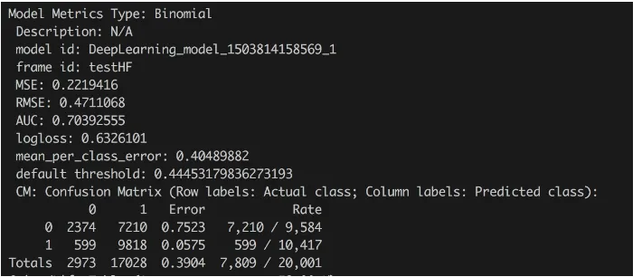
The code extracts all true negatives and positives predictions and also missed predictions and outputs of the confusion matrix based on the template shown on Figure 9:

In the preceding code, we are using a powerful Scala feature, which is called string interpolation: println(f"..."). It allows for the easy construction of the desired output by combining a string output and actual Scala variables. Scala supports different string "interporlators", but the most used are s and f. The s interpolator allows for referencing any Scala variable or even code: s"True negative: ${tn}". While, the f interpolator is type-safe - that means the user is required to specify the type of variable to show: f"True negative: ${tn}%5d" - and references the variable tn as decimal type and asks for printing on five decimal spaces.

(73)

Boson are wrongly missclassified as non-Boson. However, the overall error rate is pretty low! This is a nice example of how the overall error rate can be misleading for a dataset with an imbalanced response.

Figure 9 - Confusion matrix schema.

Next, we will consider another modeling metric used to judge classification models, called the Area Under the (Receiver Operating Characteristic) Curve (AUC) (see the following figure for an

example). The Receiver Operating Characteristic (ROC) curve is a graphical representation of the

True Positive Rate versus the False Positive Rate:

True Positive Rate: The total number of true positives divided by the sum of true positives and false negatives. Expressed differently, it is the ratio of the true signals for the Higgs-Boson particle (where the actual label was 1) to all the predicted signals for the Higgs-Boson (where our model predicted label is 1). The value is shown on the y-axis.

False Positive Rate: The total number of false positives divided by the sum of false positives and true negatives, which is plotted on the x-axis.

For more metrics, please see the figure for "Metrics derived from confusion matrix".

Figure 10 - Sample AUC Curve with an AUC value of 0.94

It follows that the ROC curve portrays our model's tradeoff of TPR against FPR for a given decision threshold (the decision threshold is the cutoff point whereby we say it is label 0 or label 1).