Subspace Pursuit for Compressive Sensing Signal
Reconstruction
Wei Dai
, Member, IEEE
, and Olgica Milenkovic
, Member, IEEE
Abstract—We propose a new method for reconstruction of sparse signals with and without noisy perturbations, termed the subspace pursuit algorithm. The algorithm has two important characteristics: low computational complexity, comparable to that of orthogonal matching pursuit techniques when applied to very sparse signals, and reconstruction accuracy of the same order as that of linear programming (LP) optimization methods. The presented analysis shows that in the noiseless setting, the pro-posed algorithm can exactly reconstruct arbitrary sparse signals provided that the sensing matrix satisfies the restricted isometry property with a constant parameter. In the noisy setting and in the case that the signal is not exactly sparse, it can be shown that the mean-squared error of the reconstruction is upper-bounded by constant multiples of the measurement and signal perturbation energies.
Index Terms—Compressive sensing, orthogonal matching pur-suit, reconstruction algorithms, restricted isometry property, sparse signal reconstruction.
I. INTRODUCTION
C
OMPRESSIVE sensing (CS) is a sampling method closely connected to transform coding which has been widely used in modern communication systems involving large-scale data samples. A transform code converts input sig-nals, embedded in a high-dimensional space, into signals that lie in a space of significantly smaller dimensions. Examples of transform coders include the well-known wavelet transforms and the ubiquitous Fourier transform.Compressive sensing techniques perform transform coding successfully whenever applied to so-called compressible and/or
-sparse signals, i.e., signals that can be represented by significant coefficients over an -dimensional basis. En-coding of a -sparse, discrete-time signal of dimension is accomplished by computing a measurement vector that con-sists of linear projections of the vector . This can be compactly described via
Here, represents an matrix, usually over the field of real numbers. Within this framework, the projection basis is
Manuscript received March 10, 2008; revised October 30, 2008. Current ver-sion published April 22, 2009. This work is supported by the National Science Foundation (NSF) under Grants CCF 0644427, 0729216 and the DARPA Young Faculty Award of the second author.
The authors are with the Department of Electrical and Computer Engi-neering, University of Illinois at Urbana-Champaign, Urbana, IL 61801-2918 USA (e-mail: [email protected]; [email protected]).
Communicated by H. Bölcskei, Associate Editor for Detection and Estima-tion.
Color versions of Figures 2 and 4–6 in this paper are available online at http:// ieeexplore.ieee.org.
Digital Object Identifier 10.1109/TIT.2009.2016006
assumed to beincoherentwith the basis in which the signal has a sparse representation [1].
Although the reconstruction of the signal from the possibly noisy random projections is an ill-posed problem, the strong prior knowledge of signal sparsity allows for recovering using projections only. One of the outstanding re-sults in CS theory is that the signal can be reconstructed using optimization strategies aimed at finding the sparsest signal that matches with the projections. In other words, the reconstruc-tion problem can be cast as an minimization problem [2]. It can be shown that to reconstruct a -sparse signal , min-imization requires only random projections when the signal and the measurements are noise-free. Unfortunately, the optimization problem is NP-hard. This issue has led to a large body of work in CS theory and practice centered around the design of measurement and reconstruction algorithms with tractable reconstruction complexity.
The work by Donoho and Candèset al.[1], [3]–[5] demon-strated that CS reconstruction is, indeed, a polynomial time problem—albeit under the constraint that more than mea-surements are used. The key observation behind these findings is that it is not necessary to resort to optimization to recover
from the underdetermined inverse problem; a much easier optimization, based on linear programming (LP) techniques, yields an equivalent solution, as long as the sampling matrix satisfies the so-called restricted isometry property (RIP) with a constant parameter.
While LP techniques play an important role in designing computationally tractable CS decoders, their complexity is still highly impractical for many applications. In such cases, the need for faster decoding algorithms—preferably operating in linear time—is of critical importance, even if one has to increase the number of measurements. Several classes of low-complexity reconstruction techniques were recently put for-ward as alternatives to LP-based recovery, which include group testing methods [6], and algorithms based on belief propagation [7].
Recently, a family of iterative greedy algorithms received sig-nificant attention due to their low complexity and simple geo-metric interpretation. They include the Orthogonal Matching Pursuit (OMP), the Regularized OMP (ROMP), and the Stage-wise OMP (StOMP) algorithms. The basic idea behind these methods is to find the support of the unknown signal sequen-tially. At each iteration of the algorithms, one or several co-ordinates of the vector are selected for testing based on the correlation values between the columns of and the regular-ized measurement vector. If deemed sufficiently reliable, the candidate column indices are subsequently added to the cur-rent estimate of the support set of . The pursuit algorithms
erate this procedure until all the coordinates in the correct sup-port set are included in the estimated supsup-port set. The compu-tational complexity of OMP strategies depends on the number of iterations needed for exact reconstruction: standard OMP al-ways runs through iterations, and therefore its reconstruc-tion complexity is roughly (see Section IV-C for details). This complexity is significantly smaller than that of LP methods, especially when the signal sparsity level is small. However, the pursuit algorithms do not have provable recon-struction quality at the level of LP methods. For OMP tech-niques to operate successfully, one requires that the correlation between all pairs of columns of is at most [8], which by the Gershgorin Circle Theorem [9] represents a more restric-tive constraint than the RIP. The ROMP algorithm [10] can re-construct all -sparse signals provided that the RIP holds with parameter , which strengthens the RIP re-quirements for -linear programming by a factor of .
The main contribution of this paper is a new algorithm, termed thesubspace pursuit(SP) algorithm. It has provable re-construction capability comparable to that of LP methods, and exhibits the low reconstruction complexity of matching pursuit techniques for very sparse signals. The algorithm can operate both in the noiseless and noisy regime, allowing for exact and approximate signal recovery, respectively. For any sampling matrix satisfying the RIP with a constant parameter inde-pendent of , the SP algorithm can recover arbitrary -sparse signals exactly from its noiseless measurements. When the measurements are inaccurate and/or the signal is not exactly sparse, the reconstruction distortion is upper-bounded by a con-stant multiple of the measurement and/or signal perturbation energy. For very sparse signals with , which, for example, arise in certain communication scenarios, the com-putational complexity of the SP algorithm is upper-bounded by , but can be further reduced to when the nonzero entries of the sparse signal decay slowly.
The basic idea behind the SP algorithm is borrowed from coding theory, more precisely, the order-statistic algorithm [11] for additive white Gaussian noise channels. In this de-coding framework, one starts by selecting the set of most reliable information symbols. This highest reliability informa-tion set is subsequently hard-decision-decoded, and the metric of the parity checks corresponding to the given information set is evaluated. Based on the value of this metric, some of the low-reliability symbols in the most reliable information set are changed in a sequential manner. The algorithm can therefore be seen as operating on an adaptively modified coding tree. If the notion of “most reliable symbol” is replaced by “column of sensing matrix exhibiting highest correlation with the vector ,” the notion of “parity-check metric” by “residual metric,” then the above method can be easily changed for use in CS recon-struction. Consequently, one can perform CS reconstruction by selecting a set of columns of the sensing matrix with highest correlation that span a candidate subspace for the sensed vector. If the distance of the received vector to this space is deemed large, the algorithm incrementally removes and adds new basis vectors according to their reliability values, until a sufficiently close candidate word is identified. SP employs a search strategy in which aconstant numberof vectors is expurgated from the
candidate list. This feature is mainly introduced for simplicity of analysis: one can easily extend the algorithm to include adaptive expurgation strategies that do not necessarily operate on fixed-sized lists.
In compressive sensing, the major challenge associated with sparse signal reconstruction is to identify in which subspace, generated by not more than columns of the matrix , the mea-sured signal lies. Once the correct subspace is determined, the nonzero signal coefficients are calculated by applying the pseu-doinversion process. The defining character of the SP algorithm is the method used for finding the columns that span the cor-rect subspace: SP tests subsets of columns in a group, for the purpose of refining at each stage an initially chosen estimate for the subspace. More specifically, the algorithm maintains a list of columns of , performs a simple test in the spanned space, and then refines the list. If does not lie in the current estimate for the correct spanning space, one refines the estimate by retaining reliable candidates, discarding the unreliable ones while adding the same number of new candidates. The “relia-bility property” is captured in terms of the order statistics of the inner products of the received signal with the columns of , and the subspace projection coefficients.
As a consequence, the main difference between ROMP and the SP reconstruction strategy is that the former algorithm gen-erates a list of candidates sequentially, without backtracing: it starts with an empty list, identifies one or several reliable candi-dates during each iteration, and adds them to the already existing list. Once a coordinate is deemed to be reliable and is added to the list, it is not removed from it until the algorithm terminates. This search strategy is overly restrictive, since candidates have to be selected with extreme caution. In contrast, the SP algo-rithm incorporates a simple method for re-evaluating the relia-bility of all candidates at each iteration of the process.
At the time of writing of this paper, the authors became aware of the related work by J. Tropp, D. Needell, and R. Vershynin [12], describing a similar reconstruction algorithm. The main difference between the SP algorithm and the CoSAMP algo-rithm of [12] is in the manner in which new candidates are added to the list. In each iteration, in the SP algorithm, only new candidates are added, while the CoSAMP algorithm adds vectors. This makes the SP algorithm computationally more effi-cient, but the underlying analysis more complex. In addition, the restricted isometry constant for which the SP algorithm is guar-anteed to converge is larger than the one presented in [12]. Fi-nally, this paper also contains an analysis of the number of itera-tions needed for reconstruction of a sparse signal (see Theorem 6 for details), for which there is no counterpart in the CoSAMP study.
Con-cluding remarks are given in Section VI, while proofs of most of the theorems are presented in the Appendix of the paper.
II. PRELIMINARIES
A. Compressive Sensing and the Restricted Isometry Property
Let denote the set of indices of the nonzero co-ordinates of an arbitrary vector , and let denote the support size of , or equivalently, its norm.1Assume next that is an unknown signal
with , and let be an observation of via linear measurements, i.e.,
where is henceforth referred to as thesampling matrix.
We are concerned with the problem of low-complexity re-covery of the unknown signal from the measurement . A nat-ural formulation of the recovery problem is within an norm minimization framework, which seeks a solution to the problem
subject to
Unfortunately, the above minimization problem is NP-hard, and hence cannot be used for practical applications [3], [4].
One way to avoid using this computationally intractable for-mulation is to consider an -minimization problem
subject to where
denotes the norm of the vector .
The main advantage of the minimization approach is that it is a convex optimization problem that can be solved efficiently by LP techniques. This method is therefore frequently referred to as -LP reconstruction [3], [13], and its reconstruction com-plexity equals when interior point methods are employed [14]. See [15]–[17] for other methods to further re-duce the complexity of -LP.
The reconstruction accuracy of the -LP method is described in terms of the RIP, formally defined below.
Definition 1 (Truncation): Let , , and
. The matrix consists of the columns of with indices , and is composed of the entries of indexed by . The space spanned by the columns of is denoted by .
Definition 2 (RIP): A matrix is said to satisfy the Restricted Isometry Property (RIP) with parameters for , , if for all index sets
such that and for all , one has
1We interchangeably use both notations in the paper.
We define , the RIP constant, as the infimum of all param-eters for which the RIP holds, i.e.,
Remark 1 (RIP and Eigenvalues): If a sampling matrix satisfies the RIP with parameters , then for all
such that , it holds that
where and denote the minimal and maximal eigenvalues of , respectively.
Remark 2 (Matrices Satisfying the RIP): Most known fam-ilies of matrices satisfying the RIP property with optimal or near-optimal performance guarantees are random. Examples in-clude the following.
1) Random matrices with independent and identically tributed (i.i.d.) entries that follow either the Gaussian dis-tribution, Bernoulli distribution with zero mean and vari-ance , or any other distribution that satisfies certain tail decay laws. It was shown in [13] that the RIP for a randomly chosen matrix from such ensembles holds with overwhelming probability whenever
where is a function of the RIP constant.
2) Random matrices from the Fourier ensemble. Here, one selects rows from the discrete Fourier transform matrix uniformly at random. Upon selection, the columns of the matrix are scaled to unit norm. The resulting matrix satisfies the RIP with overwhelming probability, provided that
where depends only on the RIP constant.
There exists an intimate connection between the LP recon-struction accuracy and the RIP property, first described by Candés and Tao in [3]. If the sampling matrix satisfies the RIP with constants , , and , such that
(1) then the -LP algorithm will reconstruct all -sparse signals exactly. This sufficient condition (1) can be improved to
(2) as demonstrated in [18].
[10]. For completeness, we include the proof of the lemma in Appendix A.
Lemma 1 (Consequences of the RIP):
1) (Monotonicity of ) For any two integers
2) (Near-orthogonality of columns) Let
be two disjoint sets, . Suppose that . For arbitrary vectors and
and
The lemma implies that , which conse-quently simplifies (1) to . Both (1) and (2) represent sufficient conditions for exact reconstruction.
In order to describe the main steps of the SP algorithm, we introduce next the notion of the projection of a vector and its residue.
Definition 3 (Projection and Residue): Let and . Suppose that is invertible. The projection of onto is defined as
where
denotes the pseudo-inverse of the matrix , and stands for matrix transposition.
Theresidue vectorof the projection equals
We find the following properties of projections and residues of vectors useful for our subsequent derivations.
Lemma 2 (Projection and Residue):
1) (Orthogonality of the residue) For an arbitrary vector , and a sampling matrix of full column rank, let . Then
2) (Approximation of the projection residue) Consider a ma-trix . Let be two disjoint sets, , and suppose that . Fur-thermore, let , , and
. Then
(3)
and
(4)
The proof of Lemma 2 can be found in Appendix B.
III. THESP ALGORITHM
The main steps of the SP algorithm are summarized below.2 Algorithm 1Subspace Pursuit Algorithm
Input: , , Initialization:
1) indices corresponding to the largest magnitude entries in the vector .
2) .
Iteration: At the th iteration, go through the following steps.
1) indices corresponding to the largest magnitude entries in the vector . 2) Set .
3) indices corresponding to the largest magnitude elements of .
4)
5) If , let and quit the iteration.
Output:
1) The estimated signal , satisfying and .
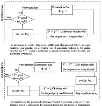
A schematic diagram of the SP algorithm is depicted in Fig. 1(b). For comparison, a diagram of OMP-type methods is pro-vided in Fig. 1(a). The subtle, but important, difference between the two schemes lies in the approach used to generate , the estimate of the correct support set . In OMP strategies, during each iteration the algorithm selects one or several indices that represent good partial support set estimates and then adds them to . Once an index is included in , it remains in this set throughout the remainder of the reconstruction process. As a result, strict inclusion rules are needed to ensure that a signifi-cant fraction of the newly added indices belongs to the correct support . On the other hand, in the SP algorithm, an estimate of size is maintained and refined during each iteration. An index, which is considered reliable in some iteration but shown to be wrong at a later iteration, can be added to or removed from the estimated support set at any stage of the recovery process. The expectation is that the recursive refinements of the estimate of the support set will lead to subspaces with strictly decreasing distance from the measurement vector .
We performed extensive computer simulations in order to compare the accuracy of different reconstruction algorithms em-pirically. In the compressive sensing framework, all sparse sig-nals are expected to be exactly reconstructed as long as the level of the sparsity is below a certain threshold. However, the com-putational complexity to test this uniform reconstruction ability is , which grows exponentially with . Instead, for em-pirical testing, we adopt the simulation strategy described in [5] which calculates theempirical frequencyof exact reconstruc-tion for the Gaussian random matrix ensemble. The steps of the testing strategy are listed as follows.
Fig. 1. Description of reconstruction algorithms forK-sparse signals: though both approaches look similar, the basic ideas behind them are quite different.
1) For given values of the parameters and , choose a signal sparsity level such that .
2) Randomly generate an sampling matrix from the standard i.i.d. Gaussian ensemble.
3) Select a support set of size uniformly at random, and generate the sparse signal vector by either one of the following two methods:
a) draw the elements of the vector restricted to from the standard Gaussian distribution; we refer to this type of signal as aGaussiansignal; or
b) set all entries of supported on to ones; we refer to this type of signal as azero–onesignal.
Note that zero–one sparse signals are of special interest for the comparative study, since they represent a particularly challenging case for OMP-type of reconstruction strate-gies.
4) Compute the measurement , apply a reconstruction algorithm to obtain , the estimate of , and compare to .
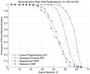
5) Repeat the process 500 times for each , and then simulate the same algorithm for different values of and . The improved reconstruction capability of the SP method, com-pared with that of the OMP and ROMP algorithms, is illustrated by two examples shown in Fig. 2. Here, the signals are drawn both according to the Gaussian and zero–one model, and the benchmark performance of the LP reconstruction technique is plotted as well.
Fig. 2 depicts the empirical frequency of exact reconstruction. The numerical values on the -axis denote the sparsity level , while the numerical values on the -axis represent the fraction of exactly recovered test signals. Of particular interest is the spar-sity level at which the recovery rate drops below 100%—i.e., thecritical sparsity—which, when exceeded, leads to errors in the reconstruction algorithm applied to some of the signals from the given class.
The simulation results reveal that the critical sparsity of the SP algorithm by far exceeds that of the OMP and ROMP tech-niques, for both Gaussian and zero–one inputs. The reconstruc-tion capability of the SP algorithm is comparable to that of the LP-based approach: the SP algorithm has a slightly higher critical sparsity for Gaussian signals, but also a slightly lower critical sparsity for zero–one signals. However, the SP algo-rithms significantly outperforms the LP method when it comes to reconstruction complexity. As we analytically demonstrate in the exposition to follow, the reconstruction complexity of the SP algorithm for both Gaussian and zero–one sparse sig-nals is , whenever , while the complexity of LP algorithms based on interior point methods is [14] in the same asymptotic regime.
IV. RECOVERY OFSPARSESIGNALS
noise-Fig. 2. Simulations of the exact recovery rate: compared with OMPs, the SP algorithm has significantly larger critical sparsity.
less setting. The techniques used in this context, and the insights obtained are also applicable to the analysis of SP reconstruction schemes with signal or/and measurement perturbations. Note that throughout the remainder of the paper, we use the nota-tion ( , ) stacked over an inequality sign to indicate that the inequality follows from Definition( ) or Lemma in the paper.
A sufficient condition for exact reconstruction of arbitrary sparse signals is stated in the following theorem.
Theorem 1: Let be a -sparse signal, and let its corresponding measurement be . If the sampling matrix satisfies the RIP with constant
then the SP algorithm is guaranteed to exactly recover from via a finite number of iterations.
Remark 3: The requirement on RIP constant can be relaxed to
if we replace the stopping criterion with . This claim is supported by substituting into (6). However, for simplicity of analysis, we adopt
for the iteration stopping criterion.
Remark 4: In the original version of this manuscript, we proved the weaker result . At the time of revision of the paper, we were given access to the manuscript [19] by Needel and Tropp. Using some of the proof techniques in their work, we managed to improve the results in Theorem 3 and therefore the RIP constant of the original submission. The in-terested reader is referred to http://arxiv.org/abs/0803.0811v2 for the first version of the theorem. This paper contains only the proof of the stronger result.
This sufficient condition is proved by applying Theorems 2 and 6. The computational complexity is related to the number of iterations required for exact reconstruction, and is discussed at the end of Section IV-C. Before providing a detailed analysis of the results, let us sketch the main ideas behind the proof.
We denote by and the residual signals based upon the estimates of before and after the th iteration of the SP algorithm. Provided that the sampling matrix satis-fies the RIP with constant (5), it holds that
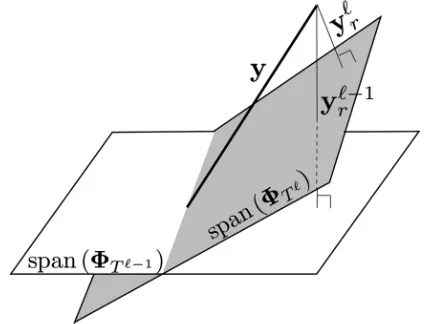
which implies that at each iteration, the SP algorithm identifies a -dimensional space that reduces the reconstruction error of the vector . See Fig. 3 for an illustration. This observation is formally stated as follows.
Theorem 2: Assume that the conditions of Theorem 1 hold. For each iteration of the SP algorithm, one has
(6) and
(7) where
(8) To prove Theorem 2, we need to take a closer look at the operations executed during each iteration of the SP algorithm. During one iteration, two basic sets of computations and com-parisons are performed: first, given , additional candi-date indices for inclusion into the estimate of the support set are identified; and second, given , reliable indices out of the total indices are selected to form . In Sections IV-A and IV–B, we provide the intuition for choosing the selection rules. Now, let be the residue signal coefficient vector corre-sponding to the support set estimate . We have the following two theorems.
Fig. 3. After each iteration, aK-dimensional hyperplane closer toyyyis ob-tained.
Theorem 3: It holds that
The proof of the theorem is postponed to Appendix D.
Theorem 4: The following inequality is valid:
The proof of the result is deferred to Appendix E.
Based on Theorems 3 and 4, one arrives at the result claimed in (6).
Furthermore, according to Lemmas 1 and 2, one has
(9) where the second equality holds by the definition of the residue, while (4) and (6) refer to the labels of the inequalities used in the bounds. In addition
(10)
Finally, elementary calculations show that when
which completes the proof of Theorem 2.
A. Why Does Correlation Maximization Work for the SP Algorithm?
Both in the initialization step and during each iteration of the SP algorithm, we select indices that maximize the cor-relations between the column vectors and the residual measure-ment. Henceforth, this step is referred to ascorrelation maxi-mization (CM). Consider the ideal case where all columns of are orthogonal.3In this scenario, the signal coefficients can
be easily recovered by calculating the correlations —i.e., all indices with nonzero magnitude are in the correct support of the sensed vector. Now assume that the sampling matrix satisfies the RIP. Recall that the RIP (see Lemma 1) implies that the columns are locally near-orthogonal. Consequently, for any not in the correct support, the magnitude of the correla-tion is expected to be small, and more precisely, upper-bounded by . This seems to provide a very simple intuition why correlation maximization allows for exact recon-struction. However, this intuition is not easy to analytically jus-tify due to the following fact. Although it is clear that for all indices , the values of are upper-bounded by , it may also happen that for all , the values of are small as well. Dealing with maximum correla-tions in this scenario cannot be immediately proved to be a good reconstruction strategy. The following example illustrates this point.
Example 1: Without loss of generality, let . Let the vectors be orthonormal, and let the remaining columns , , of be constructed randomly, using i.i.d. Gaussian samples. Consider the following normalized zero–one sparse signal:
Then, for sufficiently large
It is straightforward to envision the existence of an index , such that
The latter inequality is critical, because achieving very small values for the RIP constant is a challenging task.
3Of course, in this case no compression is possible.
This example represents a particularly challenging case for the OMP algorithm. Therefore, one of the major constraints im-posed on the OMP algorithm is the requirement that
To meet this requirement, has to be less than , which decays fast as increases.
In contrast, the SP algorithm allows for the existence of some index with
As long as the RIP constant is upper-bounded by the con-stantgiven in (5), the indices in the correct support of , that account for the most significant part of the energy of the signal, are captured by the CM procedure. Detailed descriptions of how this can be achieved are provided in the proofs of the previously stated Theorems 3 and 5.
Let us first focus on the initialization step. By the definition of the set in the initialization stage of the algorithm, the set of the selected columns ensures that
(11) Now, if we assume that the estimate is disjoint from the cor-rect support, i.e., that , then by the near orthogo-nality property of Lemma 1, one has
The last inequality clearly contradicts (11) whenever . Consequently, if , then
and at least one correct element of the support of is in . This phenomenon is quantitatively described in Theorem 5.
Theorem 5: After the initialization step, one has
and
The proof of the theorem is postponed to Appendix C. To study the effect of correlation maximization during each iteration, one has to observe that correlation calculations are performed with respect to the vector
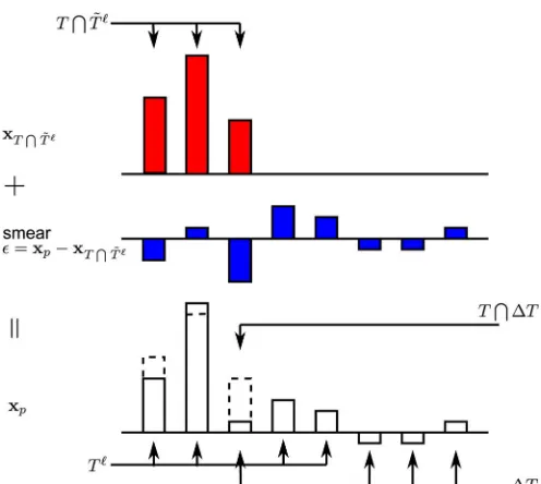
Fig. 4. The projection coefficient vectorxxx is a smeared version of the vector
xxx .
number of technical details. These can be found in the Proof of Theorem 3.
B. Identifying Indices Outside of the Correct Support Set
Note that there are indices in the set , among which at least of them do not belong to the correct support set . In order to expurgate those indices from , or equivalently, in order to find a -dimensional subspace of the space
closest to , we need to estimate these incorrect indices. Define . This set contains the indices which are deemed incorrect. If , our estimate of incorrect indices is perfect. However, sometimes . This means that among the estimated incorrect indices, there are some indices that actually belong to the correct support set . The question of interest is how often these correct indices are erroneously removed from the support estimate, and how quickly the algorithm manages to restore them back.
We claim that the reduction in the norm introduced by such erroneous expurgation is small. The intuitive expla-nation for this claim is as follows. Let us assume that all the indices in the support of have been successfully captured, or equivalently, that . When we project onto the space , it can be shown that its corresponding projection coefficient vector satisfies
and that it contains at least zeros. Consequently, the indices with smallest magnitude—equal to zero—are clearly not in the correct support set.
However, the situation changes when , or equiva-lently, when . After the projection, one has
for some nonzero . View the projection coefficient vector as a smeared version of (see Fig. 4 for illustra-tion): the coefficients indexed by may become nonzero; the coefficients indexed by may experience changes in
their magnitudes. Fortunately, the energy of this smear, i.e., , is proportional to the norm of the residual signal , which can be proved to be small according to the analysis ac-companying Theorem 3. As long as the smear is not severe, , one should be able to obtain a good estimate of via the largest projection coefficients. This intuitive ex-planation is formalized in the previously stated Theorem 4.
C. Convergence of the SP Algorithm
In this subsection, we upper-bound the number of iterations needed to reconstruct an arbitrary -sparse signal using the SP algorithm.
Given an arbitrary -sparse signal , we first arrange its el-ements in decreasing order of magnitude. Without loss of gen-erality, assume that
and that , . Define
(12) Let denote the number of iterations of the SP algorithm needed for exact reconstruction of . Then the following theorem upper-bounds in terms of and . It can be viewed as a bound on the complexity/performance tradeoff for the SP algorithm.
Theorem 6: The number of iterations of the SP algorithm is upper bounded by
This result is a combination of Theorems 7 and 8,4described
in the following.
Theorem 7: One has
Theorem 8: It can be shown that
The proof of Theorem 7 is intuitively clear and presented below, while the proof of Theorem 8 is more technical and post-poned to Appendix F.
Proof of Theorem 7: The theorem is proved by contradic-tion. Consider , the estimate of , with
Suppose that , or equivalently, . Then
However, according to Theorem 2
where the last inequality follows from our choice of such that . This contradicts the assumption and therefore proves Theorem 7.
A drawback of Theorem 7 is that it sometimes overestimates the number of iterations, especially when . The ex-ample to follow illustrates this point.
Example 2: Let , , ,
. Suppose that the sampling matrix satisfies the RIP with . Noting that , Theorem 6 implies that
Indeed, if we take a close look at the steps of the SP algorithm, we can verify that
After the initialization step, by Theorem 5, it can be shown that
As a result, the estimate must contain the index one and . After the first iteration, since
we have .
This example suggests that the upper bound (7) can be tight-ened when the signal components decay fast. Based on the idea behind this example, another upper bound on is described in Theorem 8 and proved in Appendix F.
It is clear that the number of iterations required for exact re-construction depends on the values of the entries of the sparse signal. We therefore focus our attention on the following three particular classes of sparse signals.
1) Zero–one sparse signals. As explained before, zero–one signals represent the most challenging reconstruction cat-egory for OMP algorithms. However, this class of signals has the best upper bound on the convergence rate of the SP algorithm. Elementary calculations reveal that
and that
2) Sparse signals with power-law decaying entries (also known as compressible sparse signals). Signals in this category are defined via the following constraint:
for some constants and . Compressible sparse signals have been widely considered in the CS literature, since most practical and naturally occurring signals belong to this class [13]. It follows from Theorem 7 that in this case
where when .
3) Sparse signals with exponentially decaying entries.Signals in this class satisfy
(13) for some constants and . Theorem 6 implies that
if if where again as .
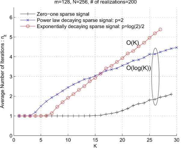
Simulation results, shown in Fig. 5, indicate that the above anal-ysis gives the right order of growth in convergence time with re-spect to the parameter . To generate the plots of Fig. 5, we set , , and run simulations for different classes of sparse signals. For each type of sparse signal, we selected dif-ferent values for the parameter , and for each , we selected 200 different randomly generated Gaussian sampling matrices and as many different support sets . The plots depict the av-erage number of iterations versus the signal sparsity level , and they clearly show that for zero–one sig-nals and sparse sigsig-nals with coefficients decaying according to a power law, while for sparse signals with expo-nentially decaying coefficients.
With the bound on the number of iterations required for exact reconstruction at hand, the computational complexity of the SP algorithm can be easily estimated: it equals the complexity of one iteration multiplied by the number of iterations. In each iteration, CM requires computations in general. For some measurement matrices with special structures, for example, sparse matrices, the computational cost can be reduced signif-icantly. The cost of computing the projections is of the order of if one uses the modified Gram–Schmidt (MGS) algorithm [20, p. 61]. This cost can be reduced further by “reusing” the computational results of past iterations within future iterations. This is possible because most practical sparse signals are compressible, and the signal support set estimates in different iterations usually intersect in a large number of indices. Though there are many ways to reduce the complexity of both the CM and projection computation steps, we only focus on the most general framework of the SP algorithm, and assume that the complexity of each iteration equals . As a result, the total complexity of the SP algorithm is given by for compressible sparse signals, and it is upper-bounded by for arbitrary sparse signals. When the signal is very sparse, in particular, when , the total complexity of SP reconstruction is upper-bounded by for arbitrary sparse signals and by for compressible sparse signals (we once again point out that most practical sparse signals belong to this signal category [13]).
The complexity of the SP algorithm is comparable to OMP-type algorithms for very sparse signals where
Fig. 5. Convergence of the subspace pursuit algorithm for different signals.
the ROMP and StOMP algorithms, the challenging signals in terms of convergence rate are also the sparse signals with ex-ponentially decaying entries. When the in (13) is sufficiently large, it can be shown that both ROMP and StOMP also need iterations for reconstruction. Note that CM operation is required in both algorithms. The total computational com-plexity is then .
The case that requires special attention during analysis is . Again, if compressible sparse signals are consid-ered, the complexity of projections can be significantly reduced if one reuses the results from previous iterations at the current it-eration. If exponentially decaying sparse signals are considered, one may want to only recover the energetically most significant part of the signal and treat the residual of the signal as noise—re-duce the effective signal sparsity to . In both cases, the complexity depends on the specific implementation of the CM and projection operations and is beyond the scope of analysis of this paper.
One advantage of the SP algorithm is that the number of iter-ations required for recovery is significantly smaller than that of the standard OMP algorithm for compressible sparse signals. To the best of the authors’ knowledge, there are no known results on the number of iterations of the ROMP and StOMP algorithms needed for recovery of compressible sparse signals.
V. RECOVERY OFAPPROXIMATELYSPARSESIGNALSFROM
INACCURATEMEASUREMENTS
We first consider a sampling scenario in which the signal is -sparse, but the measurement vector is subjected to an ad-ditive noise component, . The following theorem gives a suf-ficient condition for convergence of the SP algorithm in terms of the RIP constant , as well as an upper bounds on the re-covery distortion that depends on the energy ( -norm) of the error vector .
Theorem 9 (Stability Under Measurement Perturbations):
Let be such that , and let its corre-sponding measurement be , where denotes the noise vector. Suppose that the sampling matrix satisfies the RIP with parameter
(14) Then the reconstruction distortion of the SP algorithm satisfies
where
The proof of the theorem is given in Section V-A.
We also study the case where the signal is only approxi-mately -sparse, and the measurement is contaminated by a noise vector . To simplify the notation, we henceforth use to denote the vector obtained from by maintaining the en-tries with largest magnitude and setting all other enen-tries in the vector to zero. In this setting, a signal is said to be approxi-mately -sparse if . Based on Theorem 9, we can upper-bound the recovery distortion in terms of the and norms of and , respectively, as follows.
Corollary 1: (Stability under signal and measurement per-turbations) Let be approximately -sparse, and let . Suppose that the sampling matrix satisfies the RIP with parameter
Then
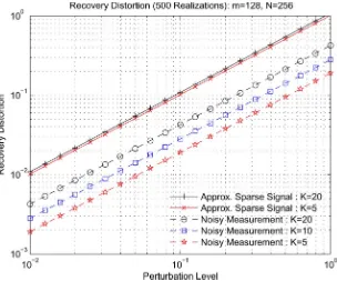
Fig. 6. Reconstruction distortion under signal or measurement perturbations: both perturbation level and reconstruction distortion are described via thel norm.
SP algorithm equals the signal sparsity level , one needs to set the input sparsity level of the SP algorithm to in order to obtain the claim stated in the above corollary.
Theorem 9 and Corollary 1 provide analytical upper bounds on the reconstruction distortion of the noisy version of the SP al-gorithm. In addition to these theoretical bounds, we performed numerical simulations to empirically estimate the reconstruc-tion distorreconstruc-tion. In the simulareconstruc-tions, we first select the dimension of the signal , and the number of measurements . We then choose a sparsity level such that . Once the param-eters are chosen, an sampling matrix with standard i.i.d. Gaussian entries is generated. For a given , the support set of size is selected uniformly at random. A zero–one sparse signal is constructed as in the previous section. Finally, either signal or a measurement perturbations are added as fol-lows.
1) Signal perturbations:the signal entries in are kept un-changed but the signal entries outside of are perturbed by i.i.d. Gaussian samples.
2) Measurement perturbations:the perturbation vector is generated using a Gaussian distribution with zero mean and covariance matrix , where denotes the
identity matrix.
We ran the SP reconstruction process on , 500 times for each , , and . The reconstruction distortion is ob-tained via averaging over all these instances, and the results are plotted in Fig. 6. Consistent with the findings of Theorem 9 and Corollary 1, we observe that the recovery distortion increases linearly with the -norm of the measurement error. Even more encouraging is the fact that the empirical reconstruction dis-tortion is typically much smaller than the corresponding upper bounds. This is likely due to the fact that, in order to simplify the expressions involved, many constants and parameters used in the proof were upper bounded.
A. Recovery Distortion Under Measurement Perturbations
The first step towards proving Theorem 9 is to upper-bound the reconstruction error for a given estimated support set , as succinctly described in the lemma to follow.
Lemma 3: Let be a -sparse vector, , and
let be a measurement for which satisfies the RIP with parameter . For an arbitrary
such that , define as
and
Then
The proof of the lemma is given in Appendix G.
Next, we need to upper-bound the norm in the th iteration of the SP algorithm. To achieve this task, we describe in the theorem to follow how depends on the RIP constant and the noise energy .
Theorem 10: It holds that
and therefore
(17) Furthermore, suppose that
(18) Then one has
whenever
Proof: The upper bounds in inequalities (15) and (16) are proved in Appendices H and I, respectively. The inequality (17) is obtained by substituting (15) into (16) as shown below:
To complete the proof, we make use of Lemma 2 stated in Sec-tion II. According to this lemma, we have
(19) and
(20) Apply the inequalities (17) and (18) to (19) and (20). Numerical analysis shows that as long as , the right-hand side of (19) is less than that of (20) and therefore . This completes the proof of the theorem.
Based on Theorem 10, we conclude that when the SP algo-rithm terminates, the inequality (18) is violated and we must have
Under this assumption, it follows from Lemma 3 that
which completes the proof of Theorem 2.
B. Recovery Distortion Under Signal and Measurement Perturbations
The proof of Corollary 1 is based on the following two lemmas, which are proved in [21] and [22], respectively.
Lemma 4: Suppose that the sampling matrix
satisfies the RIP with parameter . Then, for every , one has
Lemma 5: Let be -sparse, and let denote the vector obtained from by keeping its entries of largest mag-nitude, and by setting all its other components to zero. Then
To prove the corollary, consider the measurement vector
By Theorem 9, one has
and invoking Lemma 4 shows that
Furthermore, Lemma 5 implies that
Therefore
which completes the proof.
VI. CONCLUSION
We introduced a new algorithm, named subspace pursuit (SP), for low-complexity recovery of sparse signals sampled by matrices satisfying the RIP with a constant parameter . Also presented were simulation results demonstrating that the recovery performance of the algorithm matches, and sometimes even exceeds, that of the LP programming technique; and, simulations showing that the number of iterations executed by the algorithm for zero–one sparse signals and compressible signals is of the order .
APPENDIX
We provide next detailed proofs for the lemmas and theorems stated in the paper.
A. Proof of Lemma 1
1) The first part of the lemma follows directly from the def-inition of . Every vector can be extended to a vector by attaching zeros to it. From the fact that for all such that , and all , one has
it follows that
for all and . Since is defined as the infimum of all parameters that satisfy the above inequal-ities, .
2) The inequality
obviously holds if either one of the norms and is zero. Assume therefore that neither one of them is zero, and define
Note that the RIP implies that
(21) and similarly
We thus have
and therefore
Now
which completes the proof.
B. Proof of Lemma 2
1) The first claim is proved by observing that
2) To prove the second part of the lemma, let and
By Lemma 1, we have
On the other hand, the left-hand side of the above in-equality reads as
Thus, we have
By the triangular inequality
Finally, observing that
and , we show that
C. Proof of Theorem 5
The first step consists in proving inequality (11), which reads as
By assumption, , so that
According to the definition of
The second step is to partition the estimate of the support set into two subsets: the set , containing the indices in the correct support set, and , the set of incorrectly selected indices. Then
(22) where the last inequality follows from the near-orthogonality property of Lemma 1.
Furthermore
(23) Combining the two inequalities (22) and (23), one can show that
By invoking inequality (11) it follows that
Hence
which can be further relaxed to
To complete the proof, we observe that
D. Proof of Theorem 3
In this subsection, we show that the CM process allows for capturing a significant part of the residual signal power, that is,
for some constant . Note that in each iteration, the CM oper-ation is performed on the vector . The proof heavily relies on the inherent structure of . Specifically, in the following two-step roadmap of the proof, we first show how the measure-ment residue is related to the signal residue , and then employ this relationship to find the “energy captured” by the CM process.
1) One can write as
(24)
for some and .
Furthermore
(25) 2) It holds that
where holds because
and is a linear func-tion, follows from the fact that
, and holds by defining
As a consequence of the RIP
This proves the stated claim.
2) For notational convenience, we first define
which is the set of indices “captured” by the CM process. By the definition of , we have
(26) Removing the common columns between and
and noting that , we arrive at
(27) An upper bound on the left-hand side of (27) is given by
(28) A lower bound on the right-hand side of (27) can be derived as
(29) Substitute (29) and (28) into (27). We get
(30)
Note the explicit form of in (24). One has
(31) and
(32) From (31) and (32), it is clear that
which completes the proof.
E. Proof of Theorem 4
As outlined in Section IV-B, let
be the projection coefficient vector, and let
be the smear vector. We shall show that the smear magnitude is small, and then from this fact deduce that
for some positive constant . We proceed with es-tablishing the validity of the following three claims.
1) It can be shown that
2) Let . One has
This result implies that the energy concentrated in the er-roneously removed signal components is small.
3) Finally
Proof: The proofs can be summarized as follows. 1) To prove the first claim, note that
where the last equality follows from the definition of . Recall the definition of , based on which we have
(34) 2) Consider an arbitrary index set of cardinality
that is disjoint from
(35)
Such a set exists because . Since
we have
On the other hand, by Step 4) of the subspace algorithm, is chosen to contain the smallest projection coeffi-cients (in magnitude). It therefore holds that
(36) Next, we decompose the vector into a signal part and a smear part. Then
which is equivalent to
(37) Combining (36) and (37) and noting that
( is supported on , i.e., ), we have
(38) This completes the proof of the claimed result.
3) This claim is proved by combining (34) and (38). Since , one has
This proves Theorem 4.
F. Proof of Theorem 8
Without loss of generality, assume that
The following iterative algorithm is employed to create a par-tition of the support set that will establish the correctness of the claimed result.
Algorithm 2Partitioning of the support set Initialization:
• Let , and . Iteration Steps:
• If , quit the iterations; otherwise, continue. • If
(39) set ; otherwise, it must hold that
(40) and we therefore set and . • Increment the index , . Continue with a new
iteration.
Suppose that after the iterative partition, we have
where is the number of the subsets in the partition. Let , . It is clear that
Then Theorem 8 is proved by invoking the following lemma.
Lemma 6:
1) For a given index , let , and let
Then
for all (41) and therefore
(42) 2) Let
(43) where denotes the floor function. Then, for any
iterations, the SP algorithm has the property that
(44)
More specifically, after
(45)
iterations, the SP algorithm guarantees that .
Proof: Both parts of this lemma are proved by mathemat-ical induction as follows.
1) By the construction of
(46) On the other hand
It follows that
or, equivalently, the desired inequality (41) holds for . To use mathematical induction,supposethat for an index
for all (47) Then
This proves (41) of the lemma. Inequality (42) then follows from the observation that
2) From (43), it is clear that for
According to Theorem 2, after iterations
On the other hand, for any , it follows from the first part of this lemma that
Therefore
Now,supposethat for a given , after iterations, we have
Let . Then
Denote the smallest coordinate in by , and the largest coordinate in by . Then
After more iterations, i.e., after a total number of iter-ations equal to , we obtain
As a result, we conclude that
is valid after iterations, which proves in-equality (44). Now let the subspace algorithm run for
iterations. Then, . Finally, note that
This completes the proof of the last claim (45).
G. Proof of Lemma 3
where is a consequence of the fact that
By relaxing the upper bound in terms of replacing by , we obtain
This completes the proof of the lemma.
H. Proof of Inequality (15)
The proof is similar to the proof given in Appendix D. We start by observing that
(48) and
(49) Again, let . Then by the definition of
(50) The left-hand side of (50) is upper-bounded by
(51) Combine (50) and (51). Then
(52) Comparing the above inequality (52) with its analogue for the noiseless case, (26), one can see that the only difference is the term on the left-hand side of (52). Following the same steps as used in the derivations leading from (26) to (29), one can show that
Applying (32), we get
which proves the inequality (15).
I. Proof of Inequality (16)
This proof is similar to that of Theorem 4. When there are measurement perturbations, one has
Then the smear energy is upper-bounded by
where the last inequality holds because the largest eigenvalue of satisfies
Invoking the same technique as used for deriving (34), we have
(53) It is straightforward to verify that (38) still holds, which now reads as
(54) Combining (53) and (54), one has
which proves the claimed result.
ACKNOWLEDGMENT
REFERENCES
[1] D. Donoho, “Compressed sensing,”IEEE Trans. Inf. Theory, vol. 52, no. 4, pp. 1289–1306, Apr. 2006.
[2] R. Venkataramani and Y. Bresler, “Sub-Nyquist sampling of multiband signals: Perfect reconstruction and bounds on aliasing error,” inProc. IEEE Int. Conf. Acoustics, Speech and Signal Processing (ICASSP), Seattle, WA, May 1998, vol. 3, pp. 1633–1636.
[3] E. Candès and T. Tao, “Decoding by linear programming,”IEEE Trans. Inf. Theory, vol. 51, no. 12, pp. 4203–4215, Dec. 2005.
[4] E. Candès, J. Romberg, and T. Tao, “Robust uncertainty principles: exact signal reconstruction from highly incomplete frequency informa-tion,”IEEE Trans. Inf. Theory, vol. 52, no. 2, pp. 489–509, Feb. 2006. [5] E. Candès, R. Mark, T. Tao, and R. Vershynin, “Error correction via linear programming,” inProc. IEEE Symp. Foundations of Computer Science (FOCS), Pittsburgh, PA, Oct. 2005, pp. 295–308.
[6] G. Cormode and S. Muthukrishnan, “Combinatorial algorithms for compressed sensing,” inProc. 40th Annu. Conf. Information Sciences and Systems, Princeton, NJ, Mar. 2006, pp. 198–201.
[7] S. Sarvotham, D. Baron, and R. Baraniuk, Compressed Sensing Recon-struction Via Belief Propagation, 2006, Preprint.
[8] J. A. Tropp, “Greed is good: algorithmic results for sparse approxima-tion,”IEEE Trans. Inf. Theory, vol. 50, no. 10, pp. 2231–2242, Oct. 2004.
[9] R. S. Varga, Gerˇsgorin and His Circles. Berlin, Germany: Springer-Verlag, 2004.
[10] D. Needell and R. Vershynin, Uniform Uncertainty Principle and Signal Recovery Via Regularized Orthogonal Matching Pursuit, 2007, Preprint.
[11] Y. Han, C. Hartmann, and C.-C. Chen, “Efficient priority-first search maximum-likelihood soft-decision decoding of linear block codes,”
IEEE Trans. Inf. Theory, vol. 39, no. 5, pp. 1514–1523, Sep. 1993. [12] J. Tropp, D. Needell, and R. Vershynin, “Iterative signal recovery
from incomplete and inaccurate measurements,” inProc. Information Theory and Applications Workshop, San Deigo, CA, Feb. 2008. [13] E. J. Candès and T. Tao, “Near-optimal signal recovery from random
projections: Universal encoding strategies?,”IEEE Trans. Inf. Theory, vol. 52, no. 12, pp. 5406–5425, Dec. 2006.
[14] I. E. Nesterov, A. Nemirovskii, and Y. Nesterov, Interior-Point Polyno-mial Algorithms in Convex Programming. Philadelphia, PA: SIAM, 1994.
[15] D. L. Donoho and Y. Tsaig, Fast Solution of` -Norm Minimization Problems When the Solution May be Sparse, [Online]. Available: http://www.dsp.ece.rice.edu/cs/FastL1.pdf
[16] S.-J. Kim, K. Koh, M. Lustig, S. Boyd, and D. Gorinevsky, “A method for large-scale` -regularized least squares,”IEEE J. Sel. Topics Signal Process., vol. 1, no. 4, pp. 606–617, Dec. 2007.
[17] P. Tseng and S. Yun, “A coordinate gradient descent method for non-smooth separable minimization,”Math. Programming, vol. 117, no. 1–2, pp. 387–423, Aug. 2007.
[18] E. J. Candès, “The restricted isometry property and its implications for compressed sensing,”C. R. l’Academie des Sciences, ser. I, no. 346, pp. 589–592, 2008.
[19] D. Needell and J. A. Tropp, “Cosamp: Iterative signal recovery from in-complete and inaccurate samples,”Appl. Comp. Harmonic Anal., 2008, submitted for publication.
[20] Å. Björck, Numerical Methods for Least Squares Problems. Philadel-phia, PA: SIAM, 1996.
[21] A. Gilbert, M. Strauss, J. Tropp, and R. Vershynin, “One sketch for all: Fast algorithms for compressed sensing,” inProc. Symp. Theory of Computing (STOC), San Diego, CA, Jun. 2007, pp. 237–246. [22] D. Needell and R. Vershynin, Signal Recovery From Incomplete and
Inaccurate Measurements Via Regularized Orthogonal Matching Pur-suit, 2008, Preprint.
Wei Dai(S’01–M’08) received the Ph.D. and M.S. degree in Electrical and Computer Engineering from the University of Colorado at Boulder in 2007 and 2004, respectively.
He is currently a Postdoctoral Researcher at the Department of Electrical and Computer Engineering, University of Illinois at Urbana-Champaign. His re-search interests include compressive sensing, bioinformatics, communications theory, information theory, and random matrix theory.
Olgica Milenkovic(S’01–M’03) received the M.S. degree in mathematics and the Ph.D. degree in electrical engineering from the University of Michigan, Ann Arbor, in 2002.