Higher Engineering Mathematics
Fifth Edition
John Bird,
BSc(Hons), CMath, FIMA, FIET, CEng, MIEE, CSci, FCollP, FIIE
AMSTERDAM • BOSTON • HEIDELBERG • LONDON • NEW YORK • OXFORD PARIS • SAN DIEGO • SAN FRANCISCO • SINGAPORE • SYDNEY • TOKYO
Newnes
An imprint of Elsevier
Linacre House, Jordan Hill, Oxford OX2 8DP
30 Corporate Drive, Suite 400, Burlington, MA01803, USA First published 1993
Second edition 1995 Third edition 1999
Reprinted 2000 (twice), 2001, 2002, 2003 Fourth edition 2004
Fifth edition 2006
Copyright c2006, John Bird. Published by Elsevier Ltd. All rights reserved The right of John Bird to be indentified as the author of this work has been asserted in accordance with the Copyright, Designs and Patents Act 1998 No part of this publication may be reproduced, stored in a retrieval system or transmitted in any lausv or by any means electronic, mechanical, photocopying, recording or otherwise without the prior written permission of the publisher Permission may be sought directly from Elsevier’s Science & Technology Rights Department in Oxford, UK: phone (+44) (0) 1865 843830;
fax (+44) (0) 1865 853333; email: [email protected]. Alternatively you can submit your request online by visiting the Elsevier web site at http://elsevier.com/locate/permissions, and selectingObtaining permission to use Elsevier material
Notice
No responsibility is assumed by the publisher for any injury and/or damage to persons or property as a matter of products liability, negligence or otherwise, or from any use or operation of any methods, products, instructions or ideas contained in the material herein. Because of rapid advances in the medical sciences, in particular, independent verification of diagnoses and drug dosages should be made
British Library Cataloguing in Publication Data
A catalogue record for this book is available from the British Library Library of Congress Cataloging-in-Publication Data
A catalog record for this book is available from the Library of Congress ISBN 13: 9-78-0-75-068152-0
ISBN 10: 0-75-068152-7
For information on all Newnes publications visit our website at books.elsevier.com
Typeset by Charon Tec Ltd, Chennai, India www.charontec.com
Contents
Preface xv
Syllabus guidance xvii
Section A: Number and Algebra
1
1 Algebra 1
1.1 Introduction 1
1.2 Revision of basic laws 1 1.3 Revision of equations 3 1.4 Polynomial division 6 1.5 The factor theorem 8 1.6 The remainder theorem 10
2 Inequalities 12
2.1 Introduction to inequalities 12 2.2 Simple inequalities 12
2.3 Inequalities involving a modulus 13 2.4 Inequalities involving quotients 14 2.5 Inequalities involving square
functions 15
2.6 Quadratic inequalities 16
3 Partial fractions 18
3.1 Introduction to partial fractions 18 3.2 Worked problems on partial fractions
with linear factors 18
3.3 Worked problems on partial fractions with repeated linear factors 21 3.4 Worked problems on partial fractions
with quadratic factors 22
4 Logarithms and exponential functions 24 4.1 Introduction to logarithms 24
4.2 Laws of logarithms 24 4.3 Indicial equations 26
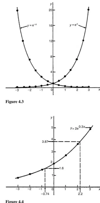
4.4 Graphs of logarithmic functions 27 4.5 The exponential function 28 4.6 The power series for ex 29
4.7 Graphs of exponential functions 31 4.8 Napierian logarithms 33
4.9 Laws of growth and decay 35 4.10 Reduction of exponential laws to
linear form 38
5 Hyperbolic functions 41
5.1 Introduction to hyperbolic functions 41 5.2 Graphs of hyperbolic functions 43 5.3 Hyperbolic identities 44
5.4 Solving equations involving hyperbolic functions 47 5.5 Series expansions for coshxand
sinhx 48 Assignment 1 50
6 Arithmetic and geometric progressions 51 6.1 Arithmetic progressions 51
6.2 Worked problems on arithmetic progressions 51
6.3 Further worked problems on arithmetic progressions 52 6.4 Geometric progressions 54 6.5 Worked problems on geometric
progressions 55
6.6 Further worked problems on geometric progressions 56
7 The binomial series 58 7.1 Pascal’s triangle 58 7.2 The binomial series 59
7.3 Worked problems on the binomial series 59
7.4 Further worked problems on the binomial series 61
7.5 Practical problems involving the binomial theorem 64
8 Maclaurin’s series 67 8.1 Introduction 67
8.2 Derivation of Maclaurin’s theorem 67 8.3 Conditions of Maclaurin’s series 67 8.4 Worked problems on Maclaurin’s
series 68
8.5 Numerical integration using Maclaurin’s series 71 8.6 Limiting values 72
9 Solving equations by iterative methods 76 9.1 Introduction to iterative methods 76 9.2 The bisection method 76
9.3 An algebraic method of successive approximations 80
9.4 The Newton-Raphson method 83
10 Computer numbering systems 86 10.1 Binary numbers 86
10.2 Conversion of binary to denary 86 10.3 Conversion of denary to binary 87 10.4 Conversion of denary to binary
via octal 88
10.5 Hexadecimal numbers 90
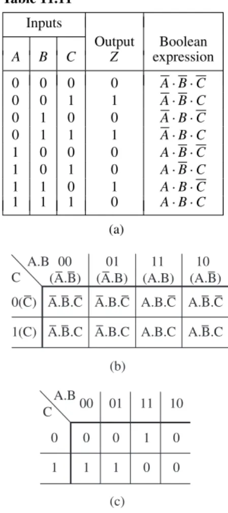
11 Boolean algebra and logic circuits 94 11.1 Boolean algebra and switching
circuits 94
11.2 Simplifying Boolean expressions 99 11.3 Laws and rules of Boolean algebra 99 11.4 De Morgan’s laws 101
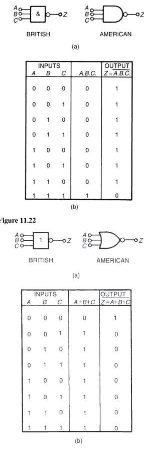
11.5 Karnaugh maps 102 11.6 Logic circuits 106 11.7 Universal logic gates 110
Assignment 3 114
Section B: Geometry and
trigonometry
115
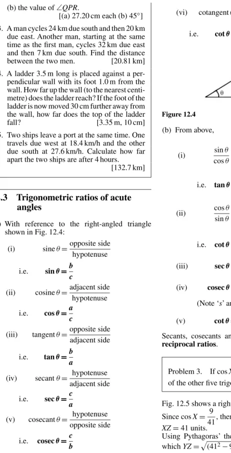
12 Introduction to trigonometry 115 12.1 Trigonometry 115
12.2 The theorem of Pythagoras 115 12.3 Trigonometric ratios of acute
angles 116
12.4 Solution of right-angled triangles 118 12.5 Angles of elevation and depression 119 12.6 Evaluating trigonometric ratios 121 12.7 Sine and cosine rules 124
12.8 Area of any triangle 125 12.9 Worked problems on the solution
of triangles and finding their areas 125 12.10 Further worked problems on
solving triangles and finding their areas 126
12.11 Practical situations involving trigonometry 128
12.12 Further practical situations involving trigonometry 130
13 Cartesian and polar co-ordinates 133 13.1 Introduction 133
13.2 Changing from Cartesian into polar co-ordinates 133
13.3 Changing from polar into Cartesian co-ordinates 135
13.4 Use ofR→PandP→Rfunctions on calculators 136
14 The circle and its properties 137 14.1 Introduction 137
14.2 Properties of circles 137
14.3 Arc length and area of a sector 138 14.4 Worked problems on arc length and
sector of a circle 139 14.5 The equation of a circle 140 14.6 Linear and angular velocity 142 14.7 Centripetal force 144
Assignment 4 146
15 Trigonometric waveforms 148
15.1 Graphs of trigonometric functions 148 15.2 Angles of any magnitude 148
15.3 The production of a sine and cosine wave 151
15.4 Sine and cosine curves 152 15.5 Sinusoidal formAsin (ωt±α) 157 15.6 Harmonic synthesis with complex
waveforms 160
16 Trigonometric identities and equations 166 16.1 Trigonometric identities 166
16.2 Worked problems on trigonometric identities 166
16.3 Trigonometric equations 167 16.4 Worked problems (i) on
trigonometric equations 168 16.5 Worked problems (ii) on
trigonometric equations 169 16.6 Worked problems (iii) on
trigonometric equations 170 16.7 Worked problems (iv) on
trigonometric equations 171
17 The relationship between trigonometric and hyperbolic functions 173
17.1 The relationship between trigonometric and hyperbolic functions 173
18 Compound angles 176
18.1 Compound angle formulae 176 18.2 Conversion ofasinωt+bcosωt
intoRsin(ωt+α) 178 18.3 Double angles 182
18.4 Changing products of sines and cosines into sums or differences 183 18.5 Changing sums or differences of
sines and cosines into products 184 18.6 Power waveforms in a.c. circuits 185
Assignment 5 189
Section C: Graphs
191
19 Functions and their curves 191 19.1 Standard curves 191 19.2 Simple transformations 194 19.3 Periodic functions 199 19.4 Continuous and discontinuous
functions 199
19.5 Even and odd functions 199 19.6 Inverse functions 201 19.7 Asymptotes 203
19.8 Brief guide to curve sketching 209 19.9 Worked problems on curve
sketching 210
20 Irregular areas, volumes and mean values of waveforms 216
20.1 Areas of irregular figures 216 20.2 Volumes of irregular solids 218 20.3 The mean or average value of
a waveform 219
Section D: Vector geometry
225
21 Vectors, phasors and the combination of waveforms 225
21.1 Introduction 225 21.2 Vector addition 225 21.3 Resolution of vectors 227 21.4 Vector subtraction 229 21.5 Relative velocity 231 21.6 Combination of two periodic
functions 232
22 Scalar and vector products 237 22.1 The unit triad 237
22.2 The scalar product of two vectors 238
22.3 Vector products 241
22.4 Vector equation of a line 245
Assignment 6 247
Section E: Complex numbers
249
23 Complex numbers 249
23.1 Cartesian complex numbers 249 23.2 The Argand diagram 250
23.3 Addition and subtraction of complex
numbers 250
23.4 Multiplication and division of complex numbers 251 23.5 Complex equations 253 23.6 The polar form of a complex
number 254
23.7 Multiplication and division in polar
form 256
23.8 Applications of complex numbers 257
24 De Moivre’s theorem 261 24.1 Introduction 261
24.2 Powers of complex numbers 261 24.3 Roots of complex numbers 262 24.4 The exponential form of a complex
number 264
Section F: Matrices and
Determinants
267
25 The theory of matrices and determinants 267
25.1 Matrix notation 267 25.2 Addition, subtraction and
multiplication of matrices 267 25.3 The unit matrix 271
25.4 The determinant of a 2 by 2 matrix 271 25.5 The inverse or reciprocal of a 2 by
2 matrix 272
25.6 The determinant of a 3 by 3 matrix 273 25.7 The inverse or reciprocal of a 3 by
3 matrix 274
26 The solution of simultaneous equations by matrices and determinants 277
26.1 Solution of simultaneous equations by matrices 277
26.3 Solution of simultaneous equations using Cramers rule 283
26.4 Solution of simultaneous equations using the Gaussian elimination
method 284
Assignment 7 286
Section G: Differential calculus
287
27 Methods of differentiation 287 27.1 The gradient of a curve 287
27.2 Differentiation from first principles 288 27.3 Differentiation of common
functions 288
27.4 Differentiation of a product 292 27.5 Differentiation of a quotient 293 27.6 Function of a function 295 27.7 Successive differentiation 296
28 Some applications of differentiation 298 28.1 Rates of change 298
28.2 Velocity and acceleration 299 28.3 Turning points 302
28.4 Practical problems involving
maximum and minimum values 306 28.5 Tangents and normals 310
28.6 Small changes 311
29 Differentiation of parametric equations 314
29.1 Introduction to parametric equations 314
29.2 Some common parametric equations 314
29.3 Differentiation in parameters 314 29.4 Further worked problems on
differentiation of parametric equations 316
30 Differentiation of implicit functions 319 30.1 Implicit functions 319
30.2 Differentiating implicit functions 319 30.3 Differentiating implicit functions
containing products and quotients 320 30.4 Further implicit differentiation 321
31 Logarithmic differentiation 324 31.1 Introduction to logarithmic
differentiation 324 31.2 Laws of logarithms 324
31.3 Differentiation of logarithmic functions 324
31.4 Differentiation of [f(x)]x 327 Assignment 8 329
32 Differentiation of hyperbolic functions 330 32.1 Standard differential coefficients of
hyperbolic functions 330 32.2 Further worked problems on
differentiation of hyperbolic functions 331
33 Differentiation of inverse trigonometric and hyperbolic functions 332
33.1 Inverse functions 332 33.2 Differentiation of inverse
trigonometric functions 332 33.3 Logarithmic forms of the inverse
hyperbolic functions 337
33.4 Differentiation of inverse hyperbolic functions 338
34 Partial differentiation 343 34.1 Introduction to partial
derivaties 343
34.2 First order partial derivatives 343 34.3 Second order partial derivatives 346
35 Total differential, rates of change and small changes 349
35.1 Total differential 349 35.2 Rates of change 350 35.3 Small changes 352
36 Maxima, minima and saddle points for functions of two variables 355 36.1 Functions of two independent
variables 355
36.2 Maxima, minima and saddle points 355 36.3 Procedure to determine maxima,
minima and saddle points for functions of two variables 356 36.4 Worked problems on maxima,
minima and saddle points for functions of two variables 357 36.5 Further worked problems on
maxima, minima and saddle points for functions of two variables 359
Section H: Integral calculus
367
37 Standard integration 367
37.1 The process of integration 367 37.2 The general solution of integrals of
the formaxn 367 37.3 Standard integrals 367 37.4 Definite integrals 371
38 Some applications of integration 374 38.1 Introduction 374
38.2 Areas under and between curves 374 38.3 Mean and r.m.s. values 376
38.4 Volumes of solids of revolution 377 38.5 Centroids 378
38.6 Theorem of Pappus 380
38.7 Second moments of area of regular sections 382
39 Integration using algebraic substitutions 391
39.1 Introduction 391
39.2 Algebraic substitutions 391 39.3 Worked problems on integration
using algebraic substitutions 391 39.4 Further worked problems on
integration using algebraic substitutions 393 39.5 Change of limits 393
Assignment 10 396
40 Integration using trigonometric and hyperbolic substitutions 397 40.1 Introduction 397
40.2 Worked problems on integration of sin2x, cos2x, tan2xand cot2x 397 40.3 Worked problems on powers of
sines and cosines 399
40.4 Worked problems on integration of products of sines and cosines 400 40.5 Worked problems on integration
using the sinθsubstitution 401 40.6 Worked problems on integration
using tanθsubstitution 403 40.7 Worked problems on integration
using the sinhθsubstitution 403 40.8 Worked problems on integration
using the coshθsubstitution 405
41 Integration using partial fractions 408 41.1 Introduction 408
41.2 Worked problems on integration using partial fractions with linear factors 408 41.3 Worked problems on integration
using partial fractions with repeated linear factors 409
41.4 Worked problems on integration using partial fractions with quadratic factors 410
42 Thet=tanθ2 substitution 413 42.1 Introduction 413
42.2 Worked problems on thet=tan θ 2 substitution 413
42.3 Further worked problems on the
t= tan θ
2 substitution 415 Assignment 11 417
43 Integration by parts 418 43.1 Introduction 418
43.2 Worked problems on integration by parts 418
43.3 Further worked problems on integration by parts 420
44 Reduction formulae 424 44.1 Introduction 424
44.2 Using reduction formulae for integrals of the form
xnexdx 424 44.3 Using reduction formulae for
integrals of the formxncosxdxand
xnsinxdx 425
44.4 Using reduction formulae for integrals of the formsinnxdxand
cosnxdx 427
44.5 Further reduction formulae 430
Section I: Differential
equations
443
46 Solution of first order differential equations by separation of variables 443
46.1 Family of curves 443 46.2 Differential equations 444
46.3 The solution of equations of the form dy
dx =f(x) 444
46.4 The solution of equations of the form dy
dx =f(y) 446
46.5 The solution of equations of the form dy
dx =f(x)·f(y) 448
47 Homogeneous first order differential equations 451
47.1 Introduction 451
47.2 Procedure to solve differential equations of the formPddyx =Q 451 47.3 Worked problems on homogeneous
first order differential equations 451 47.4 Further worked problems on
homogeneous first order differential equations 452
48 Linear first order differential equations 455
48.1 Introduction 455
48.2 Procedure to solve differential equations of the form dy
dx+Py=Q 455
48.3 Worked problems on linear first order differential equations 456 48.4 Further worked problems on linear
first order differential equations 457
49 Numerical methods for first order differential equations 460 49.1 Introduction 460 49.2 Euler’s method 460 49.3 Worked problems on Euler’s
method 461
49.4 An improved Euler method 465 49.5 The Runge-Kutta method 469
Assignment 13 474
50 Second order differential equations of the formad
2y dx2+b
dy
dx+cy=0 475
50.1 Introduction 475
50.2 Procedure to solve differential equations of the form
ad
2y
dx2+b
dy
dx+cy=0 475
50.3 Worked problems on differential equations of the form
ad
2y
dx2+b
dy
dx+cy=0 476
50.4 Further worked problems on practical differential equations of the form
ad
2y
dx2+b
dy
dx+cy=0 478
51 Second order differential equations of the formad
2y dx2+b
dy
dx+cy=f(x) 481
51.1 Complementary function and particular integral 481 51.2 Procedure to solve differential
equations of the form
ad
2y
dx2+b
dy
dx+cy=f(x) 481
51.3 Worked problems on differential equations of the formad
2y
dx2+b
dy
dx+ cy=f(x) wheref(x) is a constant or polynomial 482
51.4 Worked problems on differential equations of the formad
2y
dx2+b
dy
dx+ cy=f(x) wheref(x) is an
exponential function 484 51.5 Worked problems on differential
equations of the formad
2y
dx2+b
dy
dx+ cy=f(x) wheref(x) is a sine or cosine function 486
51.6 Worked problems on differential equations of the formad
2y
dx2+b
dy
52 Power series methods of solving ordinary differential equations 491
52.1 Introduction 491
52.2 Higher order differential coefficients as series 491
52.3 Leibniz’s theorem 493 52.4 Power series solution by the
Leibniz–Maclaurin method 495 52.5 Power series solution by the
Frobenius method 498 52.6 Bessel’s equation and Bessel’s
functions 504
52.7 Legendre’s equation and Legendre polynomials 509
53 An introduction to partial differential equations 512
53.1 Introduction 512 53.2 Partial integration 512 53.3 Solution of partial differential
equations by direct partial integration 513
53.4 Some important engineering partial differential equations 515 53.5 Separating the variables 515 53.6 The wave equation 516
53.7 The heat conduction equation 520 53.8 Laplace’s equation 522
Assignment 14 525
Section J: Statistics and
probability
527
54 Presentation of statistical data 527 54.1 Some statistical terminology 527 54.2 Presentation of ungrouped data 528 54.3 Presentation of grouped data 532
55 Measures of central tendency and dispersion 538
55.1 Measures of central tendency 538 55.2 Mean, median and mode for
discrete data 538
55.3 Mean, median and mode for grouped data 539
55.4 Standard deviation 541
55.5 Quartiles, deciles and percentiles 543
56 Probability 545
56.1 Introduction to probability 545 56.2 Laws of probability 545
56.3 Worked problems on probability 546 56.4 Further worked problems on
probability 548
Assignment 15 551
57 The binomial and Poisson distributions 553 57.1 The binomial distribution 553
57.2 The Poisson distribution 556
58 The normal distribution 559 58.1 Introduction to the normal
distribution 559
58.2 Testing for a normal distribution 563
59 Linear correlation 567
59.1 Introduction to linear correlation 567 59.2 The product-moment formula for
determining the linear correlation coefficient 567
59.3 The significance of a coefficient of correlation 568
59.4 Worked problems on linear correlation 568
60 Linear regression 571
60.1 Introduction to linear regression 571 60.2 The least-squares regression lines 571 60.3 Worked problems on linear
regression 572
Assignment 16 576
61 Sampling and estimation theories 577 61.1 Introduction 577
61.2 Sampling distributions 577 61.3 The sampling distribution of the
means 577
61.4 The estimation of population parameters based on a large sample size 581
61.5 Estimating the mean of a population based on a small sample size 586
62 Significance testing 590 62.1 Hypotheses 590
62.3 Significance tests for population
means 597
62.4 Comparing two sample means 602
63 Chi-square and distribution-free tests 607 63.1 Chi-square values 607
63.2 Fitting data to theoretical distributions 608
63.3 Introduction to distribution-free tests 613
63.4 The sign test 614
63.5 Wilcoxon signed-rank test 616 63.6 The Mann-Whitney test 620
Assignment 17 625
Section K: Laplace transforms
627
64 Introduction to Laplace transforms 627 64.1 Introduction 627
64.2 Definition of a Laplace transform 627 64.3 Linearity property of the Laplace
transform 627
64.4 Laplace transforms of elementary functions 627
64.5 Worked problems on standard Laplace transforms 629
65 Properties of Laplace transforms 632 65.1 The Laplace transform of eatf(t) 632 65.2 Laplace transforms of the form
eatf(t) 632
65.3 The Laplace transforms of derivatives 634
65.4 The initial and final value theorems 636
66 Inverse Laplace transforms 638 66.1 Definition of the inverse Laplace
transform 638
66.2 Inverse Laplace transforms of simple functions 638
66.3 Inverse Laplace transforms using partial fractions 640
66.4 Poles and zeros 642
67 The solution of differential equations using Laplace transforms 645
67.1 Introduction 645
67.2 Procedure to solve differential equations by using Laplace transforms 645
67.3 Worked problems on solving differential equations using Laplace transforms 645
68 The solution of simultaneous differential equations using Laplace transforms 650 68.1 Introduction 650
68.2 Procedure to solve simultaneous differential equations using Laplace transforms 650
68.3 Worked problems on solving simultaneous differential equations by using Laplace transforms 650
Assignment 18 655
Section L: Fourier series
657
69 Fourier series for periodic functions of period 2π 657
69.1 Introduction 657 69.2 Periodic functions 657 69.3 Fourier series 657
69.4 Worked problems on Fourier series of periodic functions of
period 2π 658
70 Fourier series for a non-periodic function over range 2π 663
70.1 Expansion of non-periodic functions 663
70.2 Worked problems on Fourier series of non-periodic functions over a range of 2π 663
71 Even and odd functions and half-range Fourier series 669
71.1 Even and odd functions 669 71.2 Fourier cosine and Fourier sine
series 669
71.3 Half-range Fourier series 672
72 Fourier series over any range 676 72.1 Expansion of a periodic function of
periodL 676
72.2 Half-range Fourier series for
73 A numerical method of harmonic analysis 683
73.1 Introduction 683
73.2 Harmonic analysis on data given in tabular or graphical form 683
73.3 Complex waveform considerations 686
74 The complex or exponential form of a Fourier series 690
74.1 Introduction 690
74.2 Exponential or complex notation 690
74.3 Complex coefficients 691 74.4 Symmetry relationships 695 74.5 The frequency spectrum 698 74.6 Phasors 699
Assignment 19 704
Essential formulae 705
Preface
This fifth edition of ‘Higher Engineering Math-ematics’ covers essential mathematical material suitable for students studying Degrees, Founda-tion Degrees, Higher NaFounda-tional Certificate and Diploma courses in Engineering disciplines.
In this edition the material has been re-ordered into the following twelve convenient categories: number and algebra, geometry and trigonometry, graphs, vector geometry, complex numbers, matri-ces and determinants, differential calculus, integral calculus, differential equations, statistics and proba-bility, Laplace transforms and Fourier series.New material has been added on inequalities, differ-entiation of parametric equations, the t=tan θ/2 substitution and homogeneous first order differen-tial equations. Another new feature is that a free Internet downloadis available to lecturers of a sam-ple of solutions (over 1000) of the further problems contained in the book.
The primary aim of the material in this text is to provide the fundamental analytical and underpin-ning knowledge and techniques needed to success-fully complete scientific and engineering principles modules of Degree, Foundation Degree and Higher National Engineering programmes. The material has been designed to enable students to use techniques learned for the analysis, modelling and solution of realistic engineering problems at Degree and Higher National level. It also aims to provide some of the more advanced knowledge required for those wishing to pursue careers in mechanical engineer-ing, aeronautical engineerengineer-ing, electronics, commu-nications engineering, systems engineering and all variants of control engineering.
In Higher Engineering Mathematics 5th Edi-tion, theory is introduced in each chapter by a full outline of essential definitions, formulae, laws, pro-cedures etc. The theory is kept to a minimum, for problem solvingis extensively used to establish and exemplify the theory. It is intended that readers will gain real understanding through seeing problems solved and then through solving similar problems themselves.
Access to software packages such as Maple, Math-ematica and Derive, or a graphics calculator, will enhance understanding of some of the topics in this text.
Each topic considered in the text is presented in a way that assumes in the reader only the knowledge attained in BTEC National Certificate/Diploma in an Engineering discipline and Advanced GNVQ in Engineering/Manufacture.
‘Higher Engineering Mathematics’ provides a follow-up to ‘Engineering Mathematics’.
This textbook contains some1000 worked prob-lems, followed by over 1750 further problems (with answers), arranged within 250 Exercises. Some 460 line diagrams further enhance under-standing.
A sample of worked solutionsto over 1000 of the further problems has been prepared and can be accessed by lecturers free via the Internet (see below).
At the end of the text, a list ofEssential Formulae is included for convenience of reference.
At intervals throughout the text are some 19 Assignmentsto check understanding. For example, Assignment 1 covers the material in chapters 1 to 5, Assignment 2 covers the material in chapters 6 to 8, Assignment 3 covers the material in chapters 9 to 11, and so on. AnInstructor’s Manual, containing full solutions to the Assignments, is available free to lecturers adopting this text (see below).
‘Learning by example’is at the heart of ‘Higher Engineering Mathematics 5th Edition’.
JOHN BIRD Royal Naval School of Marine Engineering, HMS Sultan, formerly University of Portsmouth and Highbury College, Portsmouth
Free web downloads
it is for this reason that some algebra topics – solution of simple, simultaneous and quadratic equations and transposition of formulae have been made available to all via the Internet. Also included is a Remedial Algebra Assignment to test understanding.
To access the Algebra material visit: http:// books.elsevier.com/companions/0750681527
Sample of Worked Solutions to Exercises Within the text are some 1750 further problems arranged within 250 Exercises. A sample of over 1000 worked solutions has been prepared and is available for lecturers only at http://www. textbooks.elsevier.com
Instructor’s manual
This provides full worked solutions and mark scheme for all 19 Assignments in this book,
together with solutions to the Remedial Alge-bra Assignment mentioned above. The material is available to lecturers only and is available at http://www.textbooks.elsevier.com
Syllabus guidance
This textbook is written forundergraduate engineering degree and foundation degree courses; however, it is also most appropriate forHNC/D studiesand three syllabuses are covered.
The appropriate chapters for these three syllabuses are shown in the table below.
Chapter Analytical Further Engineering
Methods Analytical Mathematics
for Methods for
Engineers Engineers
1. Algebra ×
2. Inequalities
3. Partial fractions ×
4. Logarithms and exponential functions × 5. Hyperbolic functions × 6. Arithmetic and geometric progressions ×
7. The binomial series ×
8. Maclaurin’s series ×
9. Solving equations by iterative methods × 10. Computer numbering systems × 11. Boolean algebra and logic circuits × 12. Introduction to trigonometry ×
13. Cartesian and polar co-ordinates × 14. The circle and its properties × 15. Trigonometric waveforms × 16. Trigonometric identities and equations × 17. The relationship between trigonometric and hyperbolic functions ×
18. Compound angles ×
19. Functions and their curves × 20. Irregular areas, volumes and mean value of waveforms × 21. Vectors, phasors and the combination of waveforms × 22. Scalar and vector products ×
23. Complex numbers ×
24. De Moivre’s theorem ×
25. The theory of matrices and determinants × 26. The solution of simultaneous equations by matrices ×
and determinants
27. Methods of differentiation × 28. Some applications of differentiation × 29. Differentiation of parametric equations
30. Differentiation of implicit functions × 31. Logarithmic differentiation × 32. Differentiation of hyperbolic functions × 33. Differentiation of inverse trigonometric and hyperbolic functions ×
34. Partial differentiation ×
Chapter Analytical Further Engineering
Methods Analytical Mathematics
for Methods for
Engineers Engineers
35. Total differential, rates of change and small changes × 36. Maxima, minima and saddle points for functions of two variables × 37. Standard integration ×
38. Some applications of integration × 39. Integration using algebraic substitutions × 40. Integration using trigonometric and hyperbolic substitutions × 41. Integration using partial fractions × 42. Thet= tanθ/2 substitution
43. Integration by parts ×
44. Reduction formulae ×
45. Numerical integration ×
46. Solution of first order differential equations by × separation of variables
47. Homogeneous first order differential equations
48. Linear first order differential equations ×
49. Numerical methods for first order differential equations × × 50. Second order differential equations of the ×
formad
2y
dx2 +b
dy
dx+cy=0
51. Second order differential equations of the × formad
2y
dx2 +b
dy
dx+cy=f(x)
52. Power series methods of solving ordinary × differential equations
53. An introduction to partial differential equations × 54. Presentation of statistical data ×
55. Measures of central tendency and dispersion ×
56. Probability ×
57. The binomial and Poisson distributions × 58. The normal distribution ×
59. Linear correlation ×
60. Linear regression ×
61. Sampling and estimation theories × 62. Significance testing × 63. Chi-square and distribution-free tests ×
64. Introduction to Laplace transforms × 65. Properties of Laplace transforms ×
66. Inverse Laplace transforms ×
67. Solution of differential equations using Laplace transforms × 68. The solution of simultaneous differential equations using ×
Laplace transforms
69. Fourier series for periodic functions of period 2π × 70. Fourier series for non-periodic functions over range 2π × 71. Even and odd functions and half-range Fourier series ×
72. Fourier series over any range ×
A
1
Algebra
1.1
Introduction
In this chapter, polynomial division and the fac-tor and remainder theorems are explained (in Sec-tions 1.4 to 1.6). However, before this, some essential algebra revision on basic laws and equations is included.
For further Algebra revision, go to website: http://books.elsevier.com/companions/0750681527
1.2
Revision of basic laws
(a) Basic operations and laws of indices Thelaws of indicesare:
(i) am×an=am+n (ii) a
m
an =a m−n
(iii) (am)n=am×n (iv) amn =√nam (v) a−n= 1
an (vi) a
0 =1
Problem 1. Evaluate 4a2bc3−2ac when
a=2,b= 21andc=112 4a2bc3−2ac=4(2)2
1 2
3 2
3 −2(2)
3 2
= 4×2×2×3×3×3
2×2×2×2 −
12 2 =27−6=21
Problem 2. Multiply 3x+2ybyx−y.
3x +2y x −y
Multiply byx → 3x2+2xy
Multiply by−y→ −3xy− 2y2
Adding gives: 3x2− xy−2y2
Alternatively,
(3x+2y)(x−y)=3x2−3xy+2xy−2y2
=3x2−xy−2y2
Problem 3. Simplify a
3b2c4
abc−2 and evaluate
whena=3,b= 18 andc=2.
a3b2c4 abc−2 =a
3−1b2−1c4−(−2)
=a2bc6
Whena=3,b= 18andc=2,
a2bc6=(3)21
8
(2)6=(9)1
8
(64)=72
Problem 4. Simplifyx
2y3+xy2
xy
x2y3+xy2 xy =
x2y3 xy +
xy2 xy
=x2−1y3−1+x1−1y2−1
=xy2+y or y(xy+1)
Problem 5. Simplify(x
2√y)(√x3
y2)
(x5y3)12 (x2√y)(√x3
y2)
(x5y3)12
= x
2y12x12y23
x52y32
=x2+12−52y12+23−32
=x0y−13
=y−13 or 1 y13
or 1
3
Now try the following exercise.
Exercise 1 Revision of basic operations and laws of indices
1. Evaluate 2ab+3bc−abcwhena=2,
b= −2 andc=4. [−16]
2. Find the value of 5pq2r3whenp= 25,
q= −2 andr = −1. [−8]
3. From 4x−3y+2zsubtractx+2y−3z. [3x−5y+5z] 4. Multiply 2a−5b+cby 3a+b.
[6a2−13ab+3ac−5b2+bc] 5. Simplify (x2y3z)(x3yz2) and evaluate when
x= 12,y=2 andz=3. [x5y4z3, 1312] 6. Evaluate (a32bc−3)(a21b−12c) whena=3,
b=4 andc=2. [±412]
7. Simplifya
2b+a3b
a2b2
1+a
b
8. Simplify(a
3b12c−1 2)(ab)13 (√a3√b c)
a116b13c−32 or 6
√
a11√3b
√
c3
(b) Brackets, factorization and precedence
Problem 6. Simplify
a2−(2a−ab)−a(3b+a).
a2−(2a−ab)−a(3b+a) =a2−2a+ab−3ab−a2
=−2a − 2ab or −2a(1 + b)
Problem 7. Remove the brackets and simplify the expression:
2a−[3{2(4a−b)−5(a+2b)} +4a].
Removing the innermost brackets gives: 2a−[3{8a−2b−5a−10b} +4a]
Collecting together similar terms gives: 2a−[3{3a−12b} +4a]
Removing the ‘curly’ brackets gives: 2a−[9a−36b+4a]
Collecting together similar terms gives: 2a−[13a−36b]
Removing the square brackets gives: 2a−13a+36b=−11a+36b or
36b−11a
Problem 8. Factorize (a)xy−3xz
(b) 4a2+16ab3(c) 3a2b−6ab2+15ab. (a) xy−3xz=x(y − 3z)
(b) 4a2+16ab3=4a(a + 4b3)
(c) 3a2b−6ab2+15ab=3ab(a − 2b + 5) Problem 9. Simplify 3c+2c×4c+c÷5c−8c.
The order of precedence is division, multiplication, addition and subtraction (sometimes remembered by BODMAS). Hence
3c+2c×4c+c÷5c−8c
=3c+2c×4c+c
5c
−8c
=3c+8c2+ 1
5−8c =8c2−5c+ 1
5 or c(8c − 5)+ 1 5 Problem 10. Simplify
(2a−3)÷4a+5×6−3a.
(2a−3)÷4a+5×6−3a
= 2a−3
4a +5×6−3a
= 2a−3
4a +30−3a
= 2a 4a−
3
4a+30−3a
= 1 2−
3
4a+30−3a=30 1
2 −
A
Now try the following exercise.Exercise 2 Further problems on brackets, factorization and precedence
1. Simplify 2(p+3q−r)−4(r−q+2p)+p. [−5p+10q−6r] 2. Expand and simplify (x+y)(x−2y).
[x2−xy−2y2] 3. Remove the brackets and simplify:
24p−[2{3(5p−q)−2(p+2q)} +3q]. [11q−2p] 4. Factorize 21a2b2−28ab [7ab(3ab−4)]. 5. Factorize 2xy2+6x2y+8x3y.
[2xy(y+3x+4x2)] 6. Simplify 2y+4÷6y+3×4−5y.
2
3y−3y+12
7. Simplify 3÷y+2÷y−1.
5
y −1
8. Simplifya2−3ab×2a÷6b+ab. [ab]
1.3
Revision of equations
(a) Simple equations
Problem 11. Solve 4−3x=2x−11. Since 4−3x=2x−11 then 4+11=2x+3x
i.e. 15=5xfrom which,x= 15
5 =3
Problem 12. Solve
4(2a−3)−2(a−4)=3(a−3)−1. Removing the brackets gives:
8a−12−2a+8=3a−9−1 Rearranging gives:
8a−2a−3a= −9−1+12−8
i.e. 3a= −6
and a= −6
3 =−2
Problem 13. Solve 3
x−2 = 4 3x+4.
By ‘cross-multiplying’: 3(3x+4)=4(x−2) Removing brackets gives: 9x+12=4x−8 Rearranging gives: 9x−4x= −8−12
i.e. 5x= −20
and x= −20
5 =−4
Problem 14. Solve
√
t+3 √
t
=2.
√
t
√
t+3 √
t
=2√t
i.e. √t+3=2√t
and 3=2√t−√t
i.e. 3=√t
and 9=t
(b) Transposition of formulae
Problem 15. Transpose the formula v=u+ f t
m to makef the subject.
u+f t
m =vfrom which, f t
m =v−u
and m
f t m
=m(v−u)
i.e. f t=m(v−u)
and f= m
t (v − u)
Problem 16. The impedance of an a.c. circuit is given byZ =√R2+X2. Make the reactance
√
R2+X2 =Zand squaring both sides gives
R2+X2=Z2, from which,
X2=Z2−R2andreactanceX = √Z2−R2 Problem 17. Given that D
d =
f +p f −p
, expresspin terms ofD, d andf.
Rearranging gives:
f +p f −p
= D
d
Squaring both sides gives: f +p
f −p = D2
d2
‘Cross-multiplying’ gives:
d2(f +p)=D2(f −p) Removing brackets gives:
d2f +d2p=D2f −D2p
Rearranging gives: d2p+D2p=D2f −d2f
Factorizing gives: p(d2+D2)=f(D2−d2)
and p= f(D
2−d2) (d2+D2)
Now try the following exercise.
Exercise 3 Further problems on simple equations and transposition of formulae In problems 1 to 4 solve the equations
1. 3x−2−5x=2x−4 1
2
2. 8+4(x−1)−5(x−3)=2(5−2x) [−3]
3. 1
3a−2+ 1 5a+3 =0
−18
4. 3
√
t
1−√t = −6 [4]
5. Transposey= 3(F−f) L for f.
f = 3F−yL
3 or f =F−
yL
3
6. Makelthe subject oft =2π
1
g
l= t
2g
4π2
7. Transposem= µL
L+rCR forL.
L= mrCR
µ−m
8. Makerthe subject of the formula
x y =
1+r2
1−r2 r =
x−y x+y
(c) Simultaneous equations
Problem 18. Solve the simultaneous equations:
7x−2y=26 (1)
6x+5y=29 (2)
5×equation (1) gives:
35x−10y=130 (3)
2×equation (2) gives:
12x+10y=58 (4)
equation (3)+equation (4) gives: 47x+0=188
from which, x=188
47 =4 Substitutingx=4 in equation (1) gives:
28−2y=26 from which, 28−26=2yandy=1
Problem 19. Solve
x
8+ 5
2 =y (1)
11+ y
3 =3x (2)
8×equation (1) gives: x+20=8y (3) 3×equation (2) gives: 33+y=9x (4)
A
and 9x−y=33 (6)
8×equation (6) gives: 72x−8y=264 (7) Equation (7)−equation (5) gives:
71x=284
from which, x= 284
71 =4 Substitutingx=4 in equation (5) gives:
4−8y= −20
from which, 4+20=8yandy=3
(d) Quadratic equations
Problem 20. Solve the following equations by factorization:
(a) 3x2−11x−4=0 (b) 4x2+8x+3=0
(a) The factors of 3x2 are 3x and x and these are placed in brackets thus:
(3x )(x )
The factors of−4 are+1 and−4 or−1 and+4, or −2 and +2. Remembering that the product of the two inner terms added to the product of the two outer terms must equal−11x, the only combination to give this is+1 and−4, i.e.,
3x2−11x−4=(3x+1)(x−4) Thus (3x+1)(x−4)=0 hence either (3x+1)=0 i.e.x = −13
or (x−4)=0 i.e.x = 4
(b) 4x2+8x+3=(2x+3)(2x+1) Thus (2x+3)(2x+1)=0 hence either (2x+3)=0 i.e.x= −32
or (2x+1)=0 i.e.x= −12
Problem 21. The roots of a quadratic equation are 13and−2. Determine the equation inx. If 13 and−2 are the roots of a quadratic equation then,
(x−13)(x+2)=0 i.e. x2+2x−13x− 23=0 i.e. x2+53x− 23=0
or 3x2 + 5x−2= 0
Problem 22. Solve 4x2+7x+2 = 0 giving the answer correct to 2 decimal places.
From the quadratic formula ifax2+bx+c=0 then,
x= −b±
√
b2−4ac
2a
Hence if 4x2+7x+2=0 then x= −7±
72−4(4)(2)
2(4)
= −7± √
17 8 = −7±4.123
8 = −7+4.123
8 or
−7−4.123 8 i.e. x= −0.36 or −1.39
Now try the following exercise.
Exercise 4 Further problems on simultan-eous and quadratic equations
In problems 1 to 3, solve the simultaneous equations
1. 8x−3y=51
3x+4y=14 [x=6,y= −1]
2. 5a=1−3b
2b+a+4=0 [a=2,b= −3]
3. x 5+
2y
3 =
49 15 3x
7 −
y
2+ 5
7 =0 [x=3,y=4]
4. Solve the following quadratic equations by factorization:
(a)x2+4x−32=0 (b) 8x2+2x−15=0
5. Determine the quadratic equation inxwhose roots are 2 and−5.
[x2+3x−10=0] 6. Solve the following quadratic equations,
cor-rect to 3 decimal places: (a) 2x2+5x−4=0 (b) 4t2−11t+3=0
(a) 0.637,−3.137 (b) 2.443, 0.307
1.4
Polynomial division
Before looking at long division in algebra let us revise long division with numbers (we may have forgotten, since calculators do the job for us!) For example, 208
16 is achieved as follows: 13
16208 16
48 48 — · · —
(1) 16 divided into 2 won’t go (2) 16 divided into 20 goes 1 (3) Put 1 above the zero (4) Multiply 16 by 1 giving 16 (5) Subtract 16 from 20 giving 4 (6) Bring down the 8
(7) 16 divided into 48 goes 3 times (8) Put the 3 above the 8
(9) 3×16=48 (10) 48−48=0
Hence 208
16 =13exactly
Similarly, 172
15 is laid out as follows: 11
15172 15
22 15 — 7 —
Hence 172
15 =11 remainder 7 or 11+ 7 15=11
7 15 Below are some examples of division in algebra, which in some respects, is similar to long division with numbers.
(Note that a polynomial is an expression of the form
f(x)=a+bx+cx2+dx3+ · · ·
and polynomial division is sometimes required when resolving into partial fractions—see Chapter 3)
Problem 23. Divide 2x2+x−3 byx−1. 2x2 +x −3 is called thedividend andx −1 the divisor. The usual layout is shown below with the dividend and divisor both arranged in descending powers of the symbols.
2x+3
x−12x2+ x−3 2x2−2x
3x−3 3x−3 ———
· · ———
Dividing the first term of the dividend by the first term of the divisor, i.e. 2x
2
x gives 2x, which is put
above the first term of the dividend as shown. The divisor is then multiplied by 2x, i.e. 2x(x−1)= 2x2−2x, which is placed under the dividend as shown. Subtracting gives 3x−3. The process is then repeated, i.e. the first term of the divisor,
x, is divided into 3x, giving +3, which is placed above the dividend as shown. Then 3(x−1)=3x−3 which is placed under the 3x−3. The remain-der, on subtraction, is zero, which completes the process.
Thus (2x2+x−3) ÷ (x − 1)=(2x + 3) [A check can be made on this answer by multiplying (2x+3) by (x−1) which equals 2x2+x−3]
Problem 24. Divide 3x3 + x2 + 3x + 5 by
A
(1) (4) (7)3x2−2x +5
x+13x3+ x2+3x+5 3x3+3x2
−2x2+3x+5 −2x2−2x
————– 5x+5 5x+5 ———
· · ———
(1) xinto 3x3goes 3x2. Put 3x2above 3x3
(2) 3x2(x+1)=3x3+3x2
(3) Subtract
(4) x into −2x2 goes −2x. Put −2x above the dividend
(5) −2x(x+1)= −2x2−2x
(6) Subtract
(7) xinto 5xgoes 5. Put 5 above the dividend (8) 5(x+1)=5x+5
(9) Subtract
Thus
3x3+x2+3x+5
x+1 =3x 2
− 2x + 5
Problem 25. Simplifyx
3+y3
x+y
(1) (4) (7)
x2− xy +y2 x+yx3+ 0 + 0 +y3
x3+ x2y
−x2y +y3
−x2y−xy2
————
xy2+y3 xy2+y3
——— · · ———
(1) xintox3goesx2. Putx2abovex3of dividend (2) x2(x+y)=x3+x2y
(3) Subtract
(4) xinto−x2ygoes−xy. Put−xyabove dividend
(5) −xy(x+y)= −x2y−xy2
(6) Subtract
(7) xintoxy2goesy2. Puty2above dividend (8) y2(x+y)=xy2+y3
(9) Subtract Thus
x3+y3 x+y =x
2
− xy+ y2
The zero’s shown in the dividend are not normally shown, but are included to clarify the subtraction process and to keep similar terms in their respective columns.
Problem 26. Divide (x2+3x−2) by (x−2).
x +5
x−2x2+3x− 2
x2−2x
5x− 2 5x−10 ———
8 ——— Hence
x2+3x−2
x−2 =x + 5+ 8
x − 2
Problem 27. Divide 4a3 − 6a2b + 5b3 by 2a−b.
2a2−2ab − b2
2a−b4a3−6a2b +5b3
4a3−2a2b
−4a2b +5b3
−4a2b+2ab2
————
−2ab2 +5b3
−2ab2 + b3
—————– 4b3
—————– Thus
4a3−6a2b+5b3
2a−b
=2a2 − 2ab − b2 + 4b
Now try the following exercise.
Exercise 5 Further problems on polynomial division
1. Divide (2x2+xy−y2) by (x+y).
[2x−y] 2. Divide (3x2+5x−2) by (x+2).
[3x−1] 3. Determine (10x2+11x−6)÷(2x+3).
[5x−2] 4. Find 14x
2−19x−3
2x−3 . [7x+1]
5. Divide (x3+3x2y+3xy2+y3) by (x+y). [x2+2xy+y2] 6. Find (5x2−x+4)÷(x−1).
5x+4+ 8
x−1
7. Divide (3x3+2x2−5x+4) by (x+2).
3x2−4x+3− 2
x+2
8. Determine (5x4+3x3−2x+1)/(x−3).
5x3+18x2+54x+160+ 481
x−3
1.5
The factor theorem
There is a simple relationship between the factors of a quadratic expression and the roots of the equation obtained by equating the expression to zero. For example, consider the quadratic equation
x2+2x−8=0.
To solve this we may factorize the quadratic expres-sionx2+2x−8 giving (x−2)(x+4).
Hence (x−2)(x+4)=0.
Then, if the product of two numbers is zero, one or both of those numbers must equal zero. Therefore, either (x−2)=0, from which, x=2
or (x+4)=0, from which, x= −4
It is clear then that a factor of (x−2) indicates a root of+2, while a factor of (x+4) indicates a root of−4.
In general, we can therefore say that:
a factor of (x − a) corresponds to a root ofx = a
In practice, we always deduce the roots of a simple quadratic equation from the factors of the quadratic expression, as in the above example. However, we could reverse this process. If, by trial and error, we could determine thatx=2 is a root of the equation
x2+2x−8=0 we could deduce at once that (x−2) is a factor of the expressionx2+2x−8. We wouldn’t normally solve quadratic equations this way — but suppose we have to factorize a cubic expression (i.e. one in which the highest power of the variable is 3). A cubic equation might have three simple linear factors and the difficulty of discovering all these fac-tors by trial and error would be considerable. It is to deal with this kind of case that we use the factor theorem. This is just a generalized version of what we established above for the quadratic expression. The factor theorem provides a method of factorizing any polynomial,f(x), which has simple factors.
A statement of thefactor theoremsays: ‘ifx = ais a root of the equation
f(x) = 0,then (x − a) is a factor off(x)’ The following worked problems show the use of the factor theorem.
Problem 28. Factorizex3−7x−6 and use it to solve the cubic equationx3−7x−6=0. Let f(x)=x3−7x−6
If x=1, then f(1)=13−7(1)−6= −12 If x=2, then f(2)=23−7(2)−6= −12 If x=3, then f(3)=33−7(3)−6=0 If f(3)=0, then (x−3) is a factor — from the factor theorem.
We have a choice now. We can dividex3−7x−6 by (x−3) or we could continue our ‘trial and error’ by substituting further values for x in the given expression — and hope to arrive atf(x)=0. Let us do both ways. Firstly, dividing out gives:
x2+3x +2
x−3x3−0 −7x−6
x3−3x2
3x2−7x−6 3x2−9x
———— 2x−6 2x−6 ———