Vol. 20, No. 1 (2014), pp. 11–18.
WEAK LOCAL RESIDUALS IN AN ADAPTIVE FINITE
VOLUME METHOD FOR ONE-DIMENSIONAL
SHALLOW WATER EQUATIONS
Sudi Mungkasi
1and Stephen Gwyn Roberts
21Department of Mathematics, Sanata Dharma University,
Mrican, Tromol Pos 29, Yogyakarta 55002, Indonesia, [email protected]
2Mathematical Sciences Institute, The Australian National University,
Canberra, ACT 0200, Australia, [email protected]
Abstract. Weak local residual (WLR) detects the smoothness of numerical
solu-tions to conservation laws. In this paper we consider balance laws with a source term, the shallow water equations (SWE). WLR is used as the refinement indica-tor in an adaptive finite volume method for solving SWE. This is the first study in implementing WLR into an adaptive finite volume method used to solve the SWE, where the adaptivity is with respect to its mesh or computational grids. We limit our presentation to one-dimensional domain. Numerical simulations show the effectiveness of WLR as the refinement indicator in the adaptive method.
Key words and Phrases: Finite volume methods, weak local residuals, refinement indicator, adaptive mesh refinement, shallow water equations.
Abstrak.”Residu lokal lemah” (RLL) dapat mendeteksi kehalusan solusi numerik dari hukum kekekalan. Pada makalah ini kami membahas hukum kesetimbangan dengan sebuah suku masukan, yakni persamaan air dangkal (PAD). Hal ini meru-pakan yang pertama dalam implementasi RLL untuk sebuah metode volume hingga yang adaptif untuk penyelesaian PAD, di mana adaptivitas dikaitkan dengan mesh atau grid komputasi. Bahasan dibatasi hanya untuk domain satu dimensi. Simu-lasi numerik memperlihatkan keefektifan RLL sebagai indikator penghalusan dalam metode adaptif.
Kata kunci: Metode volume hingga, residu lokal lemah, indikator penghalusan, penghalusan mesh adaptif, persamaan air dangkal.
2000 Mathematics Subject Classification: 74S10, 76M12 Received: 14-08-2013, revised: 15-01-2014, accepted: 15-01-2014.
1. Introduction
Weak local residuals as smoothness indicators for conservation laws were pro-posed by Karni, Kurganov, and Petrova [4, 5]. In their work the weak local residual (WLR) was called the weak local truncation error. In the present paper we fol-low the term “weak local residual” used by Kurganov et al. [1, 6], as this is more appropriate by definition.
Even though the corresponding theory is so far available only for scalar con-servation laws, WLR as a smoothness indicator was also valid for systems of conser-vation laws [4, 5] and even for systems of balance laws [7]. The order of accuracy of WLR in a rough region is lower than the order of accuracy in a smooth re-gion [2, 4, 5]. Therefore WLR is able to detect the smoothness of solutions.
The ability of detecting the smoothness of solutions makes the WLR a good candidate as the indicator in an adaptive numerical method to solve balance laws. So far, WLR has been implemented in adaptive numerical methods for gas dynam-ics [2, 4, 5, 6]. WLR has also been implemented in an adaptive numerical method for the shallow water equations (SWE) [1], but the adaptivity was with respect to artificial viscosity.
In this paper we implement WLR as the refinement indicator in an adaptive finite volume method used to solve the SWE. This work is the first study in im-plementing WLR into the adaptive finite volume method used to solve the SWE, where the adaptivity is with respect to its mesh or computational grids. We con-sider one-dimensional problems of water flows. We follow the frame work presented by Constantin and Kurganov [2] to compute the WLR, as it gives a simple and cheap computation of WLR. Note that an approach different from WLR is avail-able for solving SWE adaptively, such as using the Winslow’s monitor function [3] instead of WLR. However, in this paper we shall limit our presentation to WLR to solve the SWE adaptively.
This paper is organised as follows. Section 2 recalls WLR formulations for conservation laws. The WLR as the refinement indicator is implemented in an adaptive method in Section 3. Finally Section 4 draws some concluding remarks.
2. Weak Local Residuals of Conservation Laws
This section recalls the formulation of WLR based on the work of Constantin
and Kurganov [2]. We use the following conventions for our notations: xis a
one-dimesional space variable, t is the time variable,q is a conserved quantity, f is a
flux function, andq0 is an arbitrary function defined for an initial condition.
Consider the scalar conservation laws
on −∞< x < ∞, with the initial condition q(x, t) = q0(x) at t = 0. The weak
form of this initial value problem is
Z ∞
whereT(x, t) is an arbitrary test function.
Now we recall the strategy of Karni and Kurganov [4] in defining the WLR.
First we consider uniform grids. Uniform grids are taken as (xj :=j∆x,tn:=n∆t)
and letqn
j be approximate values ofq(xj, tn) computed by a conservative method.
We denote byq∆(x, t) the corresponding piecewise constant approximation,
q∆(x, t) :=qjn if (x, t)∈
This results in a cheap computation of the WLR
Ejn+1−1//22=− which can be expressed after a straightforward calculation as
Ejn+1−1//22 = ∆x
This taking linear B-splines in constructing the test function adapts from the work of Constantin and Kurganov [2] on conservation laws.
3. Weak Local Residual in An Adaptive Method
In this article we extend the implementation of WLR as the refinement indi-cator for balance laws with a nonzero source term. In particular we consider the one-dimensional shallow water equations. These equations are
ht+ (hu)x= 0, (8)
(hu)t+ hu2+12gh
2
x=−ghzx. (9)
Here, xrepresents the coordinate in one-dimensional space, t represents the time
variable, u = u(x, t) denotes the water velocity, h = h(x, t) denotes the water
height, z = z(x) is the bed topography, andg is the acceleration due to gravity.
We define stagew(x, t) asw=h+z.
Note that the WLR presented in Section 2 is defined for conservation laws. Therefore the best way to compute the WLR of the SWE is considering the mass
equation (8) with the quantity q=hand fluxf(q) =hu. The WLR based on the
mass equation for the SWE is then
Ein+1−1//22 = (1/2)
We do not consider the WLR based on the momentum equation (9). That is because the computation would require well-balanced technique, as the source term is nonzero for the momentum equation (9). The well-balanced technique for the computation of WLR is beyond the scope of this paper.
Formulation (10) is defined at each vertex and for uniform grids. To define the CK indicator at the centroid of each cell, we choose one of two available indicators at its cell vertices having the largest magnitude and divide it by the local cell width.
That is, the CK indicator at the centroid of the ith cell is
Eh,ni −1/2=
We denote by CK (Constantin-Kurganov) indicator the WLR (11) [8]. Formulation (11) can be used to compute the WLR at centroids of non-uniform cells, hence,
adaptive grids. When the numerical method has a formal order r, the order of
is O(1) near discontinuities andO ∆
min{3,r+1}
in smooth regions [2].
The order difference between discontinuous and smooth regions makes
E
able to detect the smoothness of the numerical solution.
As a test case, we recall the problem with topography considered by Felcman and Kadrnka [3]. In this test, all quantities are measured in Systeme International (SI) units and we omit the writing of the units. We consider a channel of length 25 with topography
z(x) =
0.2−0.05 (x−10)2 if 8≤x≤12,
0 5 10 15 20 25 0.0
0.2 0.4 0.6 0.8 1.0 1.2
St
ag
e
Stage Bed
0 5 10 15 20 25
0.000 0.010 0.020
C
K
0 5 10 15 20 25
Position −0.06
−0.04 −0.020.00 0.02 0.04 0.06
C
el
l l
ev
el
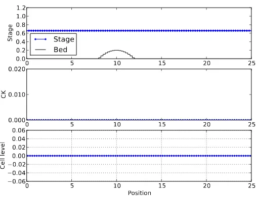
Figure 1. Initial setting for the adaptive method: water is at rest
att= 0.
and an initial condition
u(x,0) = 0, w(x,0) = 0.66 (13)
together with the Dirichlet boundary conditions
h(25, t) = 0.66, hu(0, t) =hu(25, t) = 1.53. (14)
The numerical settings are as follows. First order finite volume scheme [9] is used. The spatial domain is discretised into 100 cells initially. The tolerance of the CK indicator is
CKtol= 0.05 max|CK|, (15)
where CK is defined as in (11). Cells with |CK|>CKtol are refined binary, that
is, a “parent” cell is refined into two “children” cells with equal width. Cells with
|CK| ≤0.1 CKtol are coarsened. Two neighbouring cells are coarsened as long as
they are at the same level and have the same parent. The maximum level of binary
refinement is 10 and the width of the coarsest cell allowed is 0.25 .
Our results of the test case are as follows. The initial condition is a river at
rest with a parabolic bump at the bottom, as shown in Figure 1. For time t >0
there is a constant inflow from the left-end and constant outflow at the right-end of the domain. The inflow results in shock waves coming into the domain. The
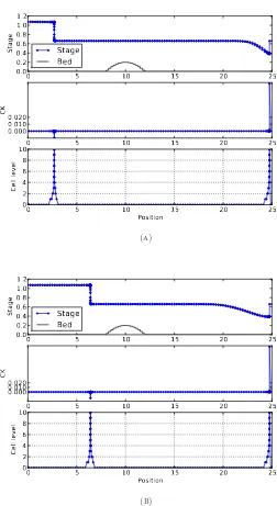
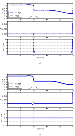
numerical results for time t > 0 are represented by Figures 2(a), 2(b) and 3(a),
which show the adaptive results at timet= 0.67, 1.67 and 2.67 respectively. Shock
0 5 10 15 20 25
Figure 2. Results produced by the adaptive method for time:
(a)t = 0.67 and (b)t = 1.67 . The flow is unsteady and moving
0 5 10 15 20 25
adaptive method involving 154 cells and (b) standard method
grid were used, the shocks could not be sharply resolved. For comparison, this result
at timet= 2.67 of the standard method is shown in Figure 3(b). We separate these
figures fromt = 0 untilt = 2.67 in order that we can clearly see the evolution of
the flow together with its mesh adaptivity and its residuals.
The adaptive strategy presented in this paper can be used to solve the one-dimensional SWE in general. The example on unsteady flow over a bump that we have discussed is a representative of one-dimensional shallow water flows.
4. Concluding Remarks
We have implemented weak local residuals as the refinement indicator in an adaptive finite volume method used to solve the shallow water equations in one dimension. The adaptivity is based on the magnitude of the residuals at each time step. Numerical results show that the coarsening and refinement can be done successfully using these weak local residuals. Possible future work is extending this technique to solve the shallow water equations in higher dimensions.
Acknowledgement. The work of Sudi Mungkasi was supported by an Australian National University (ANU) Postdoctoral Fellowship. This work was done partly when he was a doctoral student at the ANU under the supervision of Stephen Roberts.
References
[1] Chen, Y., Kurganov, A., Lei, M., and Liu, Y., “An adaptive artificial viscosity method for the Saint-Venant system”, Notes on Numerical Fluid Mechanics and Multidisciplinary Design,
120(2012), 125–141.
[2] Constantin, L.A., and Kurganov, A., “Adaptive central-upwind schemes for hyperbolic sys-tems of conservation laws”, in Hyperbolic problems: Theory, numerics, and applications, Volume 1 (F. Asakura et al., editors), Yokohama Publishers, Yokohama, 2006, pages 95–103. [3] Felcman, J., and Kadrnka, L., “Adaptive finite volume approximation of the shallow water
equations”,Applied Mathematics and Computation,219(2012), 3354–3366.
[4] Karni, S., and Kurganov, A., “Local error analysis for approximate solutions of hyperbolic conservation laws”,Advances in Computational Mathematics,22(2005), 79–99.
[5] Karni, S., Kurganov, A., and Petrova, G., “A smoothness indicator for adaptive algorithms for hyperbolic systems”,Journal of Computational Physics,178(2002), 323–341.
[6] Kurganov, A., and Liu, Y., “New adaptive artificial viscosity method for hyperbolic systems of conservation laws”,Journal of Computational Physics,231(2012), 8114–8132.
[7] Mungkasi, S., Li, Z., and Roberts, S. G., “Weak local residuals as smoothness indicators for the shallow water equations”,Applied Mathematics Letters,30(2014), 51–55.
[8] Mungkasi, S., and Roberts, S. G., “Numerical entropy production for shallow water flows”, ANZIAM Journal,52(2011), C1–C17.