1
A fuzzy vendor managed inventory of multi-item economic order quantity
model under shortage: An ant colony optimization algorithm
Ali Roozbeh Nia, Ph.D. student
Young Researchers Club, Qazvin Branch, Islamic Azad University, Qazvin , Iran Phone : +98 (281) 3665275, Fax : +98 (281) 3665277, e-mail:ali.roozbehnia@gmail.com
Mohammad Hemmati Far, Ph.D. student
Department of Industrial & Mechanical Engineering, Islamic Azad University, Qazvin Branch, Qazvin, Iran Phone : +98 (281) 3665275, Fax : +98 (281) 3665277, e-mail: m.hemmatifar@gmail.com
Seyed Taghi Akhavan Niaki, Ph.D.
Department of Industrial Engineering, Sharif University of Technology, Tehran, Iran
Phone: +98 21 66165740, Fax: +98 21 66022702, e-mail: niaki@sharif.edu
Abstract
In this study, a multi-item economic order quantity model with shortage under vendor managed inventory policy in a single vendor single buyer supply chain is developed. This model explicitly includes warehouse capacity and delivery constraints, bounds order quantity, and limits the number of pallets. Not only the demands are considered imprecise, but also resources such as available storage and total order quantity of all items can be vaguely defined in different ways. An ant colony optimization is employed to find a near-optimum solution of the fuzzy nonlinear integer-programming problem with the objective of minimizing the total cost of the supply chain. Since no benchmark is available in the literature, a genetic algorithm is developed as well to validate the result obtained. Furthermore, the applicability of the proposed methodology along with a sensitivity analysis on its parameter is shown by four numerical examples containing different numbers of items. Keywords: Ant colony optimization; Economic order quantity; Fuzzy
nonlinear integer programming; Genetic algorithm; Vendor managed inventory
2 1. Introduction
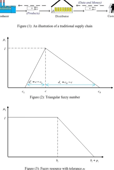
Supply chain (SC) management is the management of material and information flows both in and between facilities, such as vendors, manufacturing and assembly plants, and distribution centers (Thomas & Griffin, 1996). With the emergence of international markets and the growth of globalization, the management of supply chains has gained increased attention. The high complexity of the underlying procurement, production and distribution processes, as well as the increasing number of parties involved, create the necessity for efficient decision support systems (Schmid et al., 2013). Some inventory policies such as economic order quantity (EOQ) and economic production quantity (EPQ) are usually adopted in SCs. A century ago, Harris (1913) proposed the EOQ model and five years later, Taft (1918) recommended the EPQ inventory model; both without backorders. Later, Hadley & Whitin (1963) proposed the EOQ/EPQ inventory model with backorders. A complete review of different optimization methods used in inventory field can be seen in Cárdenas-Barrón (2011).
3
Insert Figure (1) about here
There is an abundant literature that models uncertainty in demand and/or lead time using probability distributions with known parameters. However, in many cases where there is little or no historical data available to the inventory decision maker, perhaps due to recent changes in the SC environment, probability distributions may simply not be available, or may not be easily or accurately estimated (Xie et al., 2006). Additionally, in some cases, it may not be possible to collect data on the random variables of interest because of certain system or time constraints. Furthermore, other critical SC parameters, in particular the various costs that impact the system, are often ill-defined and may vary from time to time. All of these situations raise challenges for using traditional inventory models in practice. Fuzzy theory provides an alternate, flexible approach to handle such situations because it allows the model to easily incorporate various experts’ advice in developing critical parameter estimates (Zimmermann, 2001). Fuzzy sets are introduced to avoid imprecise deliveries, orders and demands within SCs and they out-perform traditional VMI by Bullwhip effect and inventory declines (Lin et al., 2010). Adaptive fuzzy VMI control can always provide 100% service levels by adaptively responding to the demand changes according to production capacity, available stock and shortages (Kristianto et al., 2012).
While a substantial amount of research works are available in the literature, a brief review of the works on the fuzzy traditional and fuzzy VMI SC is presented in the next section.
2. Literature review
A brief review of the literature is given on the fuzzy traditional and fuzzy VMI SC inventory in the next two subsections.
2.1. Fuzzy traditional SC and inventory models
4
minimization and imprecise constraints on warehouse space and number of production runs with crisp/imprecise inventory costs. In their work, the fuzzy inventory model has been formulated into a fuzzy non-linear decision making problems and was solved by both genetic algorithm (GA) and fuzzy non-linear programming (FNLP) method based on Zimmermann’s approach. Their model was illustrated numerically and the results from different methods were compared. Wang & Shu (2005) proposed a fuzzy decision methodology that provides an alternative framework to handle SC uncertainties and to find out SC inventory strategies, while there is lack of certainty in data or even lack of available historical data.
Aliev et al. (2007) pointed out that we are usually faced with uncertain market demands and capacities in production environment, imprecise process times, and other factors introducing inherent uncertainty to the solution. In their research, they investigates a fuzzy production–distribution aggregate planning problem in SC and formulated it into a fuzzy programming model with the solution obtained by GA. Alex (2007) provided a novel approach to model uncertainties involved in the SC management using the fuzzy point estimation. Selim et al. (2008) adopted different fuzzy programming approaches for the collaborative production–distribution planning problems in different SC structure. Besides, in a non-fuzzy environment, Pasandideh et al. (2011) presented a GA for a VMI SC with several products and constraints based on EOQ with backorders considering two classical backorders costs of linear and fixed.
2.2. Fuzzy VMI supply chain
Although the VMI SC system in a fuzzy environment is closer to reality and is more applicable compared to the one used under non-fuzziness, to the best of authors’ knowledge, there are just two research works that adopt fuzziness, but with the focus of reducing the Bullwhip effect. Lin et al. (2010) applied fuzzy arithmetic operations in a VMI SC with fuzzy demands. The application pays attention to the ordering process and controlling the buyer’s target inventory level. Kristianto et al. (2012) proposed an adaptive fuzzy control application to produce an adaptive smoothing constant in the forecast method, production and delivery plan to remove, for example, the rationing and gaming or the Houlihan effect and the order batching effect or the Burbidge effects and finally the Bullwhip effect. The results showed that the adaptive fuzzy VMI control surpasses fuzzy VMI control and traditional VMI in terms of mitigating the Bullwhip effect and lower delivery overshoots and backorders.
5
from a traditional SC model offered by Taleizadeh et al. (2012) to develop a fuzzy multi-item multi-constraint EOQ model with shortage under VMI policy in a single-vendor single-buyer SC. Moreover, to bring the model to be applicable to closer to reality problems, additional contractual agreement between the vendor and the buyer including constraints on the number of pallets required to deliver the items, number of deliveries, and quantity of an order under fuzzy environment are considered. In this work not only the storage capacity and the total order quantity of all items, but also demands are considered fuzzy. In addition, an ant colony optimization (ACO) is employed to find a near-optimum solution of the fuzzy nonlinear integer-programming (FNIP) problem with the objective of finding the products' orders quantities, their required number of pallets and their maximum backorder levels per cycle; in order to minimize the total fuzzy VMI inventory cost while the constraints are satisfied. Since no benchmark is available in the literature, a genetic algorithm and a differential evolution (DE) are developed as well to validate the result obtained. Furthermore, the applicability of the proposed methodology along with a sensitivity analysis on its parameter is shown using five numerical examples containing different numbers of items. In short, the highlights of the differences of this research with the previous studies are as follow:
Considering fuzzy environment and VMI supply chain simultaneously
Adding a VMI contractual agreement between the supplier and the buyer to make the model more applicable
Proposing a new modeling to the fuzzy VMI problem with multi items and shortage
In this work not only storage capacity and total order quantity of all items but also demand are considered fuzzy
Employing three meta-heuristic algorithms (ACO, GA, and DE) to solve a FNIP problem.
Providing a case study in an Iranian automobile SC (the SAPCO Company) to apply the proposed model. SAPCO interacts with over 500 part-manufacturers to utilize the VMI policy. It is one of the main companies of SAIPA holding that produces a full series of vehicles including cars, pick-ups, 4WDs, light and heavy commercial vehicles, vans, and buses.
6
analysis on its parameter, five numerical examples including different numbers of items are solved in Section 6. Finally, conclusions and future research topics are provided in Section 7.
3. The problem and the assumptions
In a single-supplier single-buyer SC that utilizes the VMI policy, the supplier’s information system directly receives consumer demand data. As a result, the supplier has now the combined inventory with order setup and holding cost (Dong & Xu 2002). Unlike the traditional system, the supplier and the buyer in a VMI system act as a single unit. They work based on an agreement which is admitted by both parties. This alliance is the main idea of VMI and declares that the supplier establishes and manages the inventory control policies. In this circumstance, it is assumed that the supplier pays the ordering and holding costs on behalf of the buyer as a part of the mentioned agreement; the buyer paying no cost. This assumption has also been taken into considerations in prior research works such as Yao et al. (2007), Razemi et al. (2010), Pasandideh et al. (2010), and Pasandideh et al. (2011) where SC integration based on the VMI policy has been discussed.
This research is concerned with a SC providing several items using the EOQ model in which not only there are limited storage capacity and budget, but also order quantities are limited and depend on the pallet capacity. Further, shortages are allowed in the form of backorders, where a linear backorder cost per unit per time unit is applied to all items (Cardenas-Barron et al. 2012). Since the demands are rarely imprecise in real world supply chains, triangular or trapezoidal fuzzy numbers are assumed to model imprecision and to bring the model to be more applicable. Moreover, resources such as available storage, total order quantity of all items, and budget may also be vague, and hence can be modeled as fuzzy numbers. The objective is to find the items' order quantities, their required number of pallets, and their maximum backorder levels per cycle such that the total fuzzy VMI inventory cost is minimized while the constraints are satisfied.
3.1. Assumptions
The following assumptions are made to formulate the problem mathematically: a) There is a single supplier, single buyer SC with n items
b) Shortage is allowed in the form of backorder for all items
7
e) Orders are delivered by pallets and are assumed instantaneous (lead time is assumed zero)
f) Quantity discount is not allowed
g) The price for all items is fixed in the planning period h) The production rate for all items is infinite (EOQ model)
i) Costumer’s demand for all items is fuzzy (Triangular fuzzy number) j) The storage capacity is limited and fuzzy
k) The buyer's total order quantity of all items is limited and fuzzy l) The buyer's order quantity of an item has a lower and an upper bound
m) The order quantity of each item is constrained (depends on the pallet’s capacity) n) The number of pallets for an item is limited.
4. Mathematical model
Before giving the mathematical formulation of the problem at hand, the notations are first introduced in Subsection 4.1. Then, a crisp version of the problem is modeled in Subsections 4.2 to 4.6.
4.1. Notations
For j 1 2, ,..., n, let define the parameters and the variables of the model as:
:
n Number of items
j
Q : Order quantity of item j (a decision variable)
j
L : Lower limit on the order quantity of item j
j
U : Upper limit on the order quantity of item j
j
D : Buyer's fuzzy demand rate of item j jS
A : Supplier’s fixed ordering cost per ordered unit of item j jB
A : Buyer's fixed ordering cost per ordered unit of item j jB
h : Holding cost per unit of item j held in buyer's store in a period j
b : Maximum backorder level of item j in a cycle of the VMI chain (a decision
variable)
1
: Fixed backorder cost per unit (time independent)
2
8 :
j
f Space occupied by each unit of item j
:
F Fuzzy available storage space for all items with tolerance P 1
V: Fuzzy upper bound on total order quantity of all items with tolerance P 2 j
K : Capacity of the pallet for item j j
N : Number of pallets for an order of item j (a decision variable)
j
M : Upper limit on the number of pallets for each order of item j
( j)
TC O : Total ordering cost
( j)
TC H : Total holding cost ( )j
TC b : Total shortage cost
( VMI)
TC B : Total cost of Buyer's inventory in the VMI chain ( VMI)
TC S : Total cost of Supplier's inventory in the VMI chain
VMI
TC : Crisp total costs of the VMI chain
Based on the above definitions, the mathematical model of the crisp problem is derived in the next subsections.
4.2. The buyer's total cost
In the SC under the VMI policy, the supplier based on his own inventory cost (which equals to the total cost of the SC,) determines the timing and the quantity of production in a cycle. The major difference between not using and using VMI is that the supplier determines the buyer's order quantity in a VMI policy, where it is assumed that the supplier on behalf of the buyer pays the ordering and the holding cost (Razemi et al. 2010; Pasandideh et al. 2011). Thus, the buyer pays no cost and we have
0
VMI
TB (1)
4.3. The supplier's total cost
In EOQ model with shortage under the VMI policy, the supplier total cost per unit time of the jthitem is determined by adding the cost of ordering, holding, and shortage as
( VMI) ( j) ( j) ( )j
TC S TC O TC H TC b (2)
9
As a result, the supplier's total cost becomes (Pasandideh et al. 2011),
24.4. The chain total cost
Based on Eq. (1) and (6), the total cost of the SC under the VMI policy is determined by
As mentioned previously, there is a contractual agreement between the supplier and the buyer that makes the constraints of the model. The vendor storage capacity is limited and since the average inventory of the jthitem is
Qj bj
, the space constraint will be (Cardenas-Barron et al. 2012; Pasandideh et al. 2011),
Moreover, the bounds on the buyer's order quantity of the jthitem are (Darvish & Odah, 2010),
j j j
L Q U (9)
In addition, the buyer's total order quantity of all items is limited to V , that is
10
Finally, the maximum backorder level of item j in a cycle must be less than or equal to its
order quantity. That is
j j
b Q (13)
4.6. The final crisp model
Based on Equations (7)-(13), the multi-item multi-constraint EOQ model under VMI policy can be easily obtained as
2 VMI policy given in (14) is minimized and all the constraints are fulfilled. This model contains 3n discrete variables that make the optimization problem hard to solve. Thedifficulty originates from the quantity of discrete variables and the nonlinearity of the objective function and constraint in the NIP formulation.
11
4.7. The fuzzy inventory model
As mentioned previously, in this research a fuzzy and a closer to reality situation is considered for the crisp problem modeled in (14). In addition, in order the SC decision makers to draw ultimate conclusions; the fuzzy result is to be converted into a crisp value, the process of which known as defuzzification. Zimmerman (1976, 1985) developed a tolerance approach to transform a fuzzy decision making problem to regular crisp optimization problem and showed that it can be solved to obtain a unique exact optimal solution with highest membership degree using classical optimization algorithm. While many methods for defuzzificatin of fuzzy numbers can be utilized, one of the most commonly employed one namely the first index proposed by Yager (1979, 1981) is used in this paper, where two methods for defuzzification of fuzzy resources and demands are adopted as explained in the next two subsections.
4.7.1. The linear ranking function method
A general problem with fuzzy objective coefficients is formulated as follows ( )
where x is an n-dimensional solution vector, b is the constrained resources, i m is the
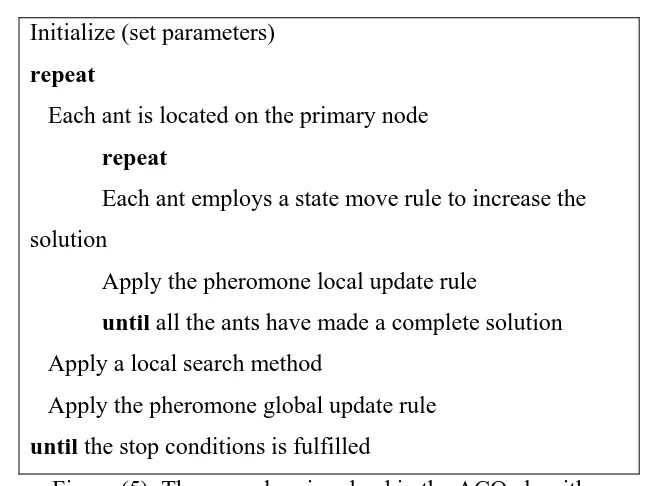
number of constraints and the symbol ‘~’ represents the fuzziness of the parameter. Assuming triangular fuzzy numbers cT ( , ,c c cL R), the problem defined in (15) is transformed into its crisp equivalent as (Yager 1979, 1981):
( ) ( )
where d and c dc are the lateral margins (right and left, respectively) of the triangular fuzzy number central point c(see Fig. 2).
Insert Figure (2) about here
4.7.2. The Zimmerman method
12
In addition, let the membership functions of the fuzzy sets representing the fuzzy constraints be defined as
where p is the tolerance of problem resources (see Fig. 3). The membership function of the i
objective function can be determined by solving the following two models: ( )
where the minimum total cost, ( )f x opt, in the model with and without tolerance for resources is f and 0 f , respectively. The membership function of the objective function is therefore 1
1
With the above settings, the fuzzy problem is transformed to a crisp nonlinear programming problem as
13
4.8. The proposed fuzzy model
Based on the backgrounds given in Subsections 4.7.1 and 4.7.2, when the demand, the available storage, and the total order quantity of all items are fuzzy, the model in (14) is transformed to
14
d are the lateral margins (right and left, respectively) of the triangular fuzzy number central point D .j Based on Zimmerman’s (1976, 1985) method for resource defuzzification, the fuzzy model in (24) is converted to its equivalent crisp decision making problem as
target, i.e., aspiration level of the objective function.
In the next section, a meta-heuristic solution algorithm is proposed to efficiently solve the problem.
5. The solution algorithm
15
integer nonlinear optimization is one of the most difficult problems in practical optimization. In other words, the objective function has a non-derivative structure, the decision variables are integer, and exact methods are costly to be employed. Hence, a meta-heuristic search algorithm is needed for a near-optimum solution. Many researchers have successfully used meta-heuristic approaches to solve complicated optimization problems in various fields of scientific and engineering disciplines. Some of these meta-heuristic algorithms are:
Genetic algorithm (Al-Tabtabai & Alex 1999; Passandideh et al. 2011; Shahsavar et al. 2010),
Ant colony optimization (Colorni et al. 1994; Dorigo & Stutzle 2004),
Simulating annealing (Aarts & Korst 1989; Taleizadeh et al. 2008),
Particle swarm optimization (Alfi & Fateh 2011; Hosseini et al. 2009; Kaveh & Laknejadi 2011; Taleizadeh et al. 2010),
Threshold accepting (Dueck & Scheuer 1990),
Tabu search (Joo & Bong 1996),
Neural networks (Abbasi & Mahlooji 2012),
Evolutionary algorithm (Laumanns et al. 2002; Taleizadeh et al. 2009),
Harmony search (Jaberipour & Khorram 2011; Kaveh & Ahangaran 2012).
Differential evolution (Lee et al 2011; Liao 2010; Huang 2007; Becerra & Coello 2006; Liu 2010).
Population-based algorithms are commonly preferred to others and in some cases
show superior performances. Consequently, an ant colony algorithm is utilized in this research in order to solve the formulated problem in (25). In addition, two other meta-heuristic algorithms of GA and DE are employed as well to enable validating the results obtained.
In the next tow subsections, brief descriptions are first given for ant colony, genetic algorithm, and differential evolution. Then, in the subsequent subsection, the steps involved in the proposed solution methods are described.
5.1. Ant Colony Optimization
16
with many problems in real world environments. In what follows, we briefly review the basis of ACO employed to find a near optimum solution to (25).
The notion behind ACO is based on the ‘‘natural’’ algorithm used by real ants to generate a near-optimal path between their nest and the food source, as shown in Fig. 4. During their seeking food process, ants deposit chemical substances called pheromones on their way back to their nest. Other ants sense the pheromone and are highly interested to the marked paths; the more pheromone that is released on a path, the more attractive that path becomes. The pheromone vapors and vanishes over time. Evaporation removes the pheromone on longer paths (and also on less interesting paths). Shorter paths are refreshed more rapidly, therefore having the chance of being more frequently explored. Naturally, ants will join towards the most efficient path due to the fact that it gets the strongest density of pheromone. The concept of the ACO algorithm is to mimic this performance. This simulation is achieved by creating a pheromone matrix n×m, employed by two key operations: the pheromone quantity tuning (also identified as pheromone deposit and pheromone evaporation
rules) and a probabilistic rule that selects an endpoint based on the pheromone quantity (the
state transition rule).
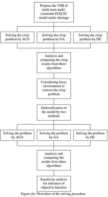
The procedure of the ACO algorithm is displayed in Fig. 5. In this algorithm, m ants are employed in each cycle, to make a full solution. To complete this task, the solution is obtained in steps. To define each step, two rules are used, as
* 0
S is a path chosen according to the probability given in (27),
q is a uniform random value between 0 and 1,
0 q0 1 is a parameter chosen during the implementation of the algorithm
17
p denotes the probability of ant r in node i to choose node j,
( , )i j is the pheromone path value between nodes i and j,
( , )i j is a heuristic value used as the visibility from node i to node j.
In addition, two updated rules are used: the first is the evaporation of the existing pheromone; the second is the quantity of added pheromone on the path. These rules are presented in Eqs. (28) and (29)
1
L shows how much the pheromone path should increase. r
0 1 is the evaporation parameter.
Insert Figure (4) about here Insert Figure (5) about here
5.2. Genetic Algorithm
In this paper, a GA is also developed for NIP problems with fuzzy demand and resources. The main parameters of a GA are the population size NGA , the crossover probabilityP , and the mutation probabilityc P (where the probability of reproduction is m
1
E C m
P ( P P )). The GA parameters of this research take three different values, based on which the best combination is selected. The stopping criterion is 200 iterations. Moreover, the steps involved in the proposed real coded GA algorithm are:
1. Set the parametersP , c P and m NGA
2. Initialize the population randomly
18
4. Select individuals for mating pool (The individuals with higher membership degree have higher probability to reproduce children)
5. Apply the crossover operation for each pair of chromosomes with probability P c
6. Apply the mutation operation for each chromosome with probability P m
7. Replace the current population by the resulting mating pool 8. Evaluate the fitness function
9. If stopping criterion is met stop. Otherwise, go to Step 5.
5.3. Differential evolution
Storn & Price (1997) were the first who introduced differential evolution (DE) to solve optimization problems. At its origin, DE was intended for continuous optimization problems without constraints. However, its present extensions can handle problems of mixed variables and can manage non-linear constraints. Currently, an important number of industrial and scientific applications make use of DE. DE sequentially uses mutation, crossover, and selection operators to produce offspring.
Let DE have a population of NP individuals at generation t, pt
p p1t, t2,...,ptNP
, wherep is an individual defined by it pit
x xit1, it2,...,xiDt
, (i=1,2,…,NP), tij
x (j=1,2,…,D) is a gene of an individual, and D is the number of genes of an individual.
Mutation: In the mutation process, DE creates a mutant vector
1, 2,...,
t t t t
i i i iD
v v v v for
each individual pitcalled a target vector. There are five representative and widely
used mutation operators in the literature, i.e., rand/1, best/1, current-to-best/ 1, best/2, and rand/2. They are respectively described as
1 .( 2 3)
toNP, and pbestt is the best individual in the current population. In this study, the best/2
19
Crossover: Following the mutation, a trail vector
1, 2,...,
t t t t
i i i iD
u u u u is produced using the following crossover operator
, if (0,1) uniformly distributed random number between 0 and 1.
Selection: Subsequently DE chooses the better one from the trail vector uit and the target vector pit to be an individual in the next generation by usually applying the following selection operator
5.4. The steps involved in the solution procedure
The main steps in the proposed procedure are as follow:
Step1: Determine the total cost of all items using the crisp model shown in (14) using ACO, GA, and DE.
Step2: Determine the total cost of all items in fuzzy model (25) by ACO, GA, and DE.
Step3: Perform sensitivity analysis on the tolerance of the objective function (p0) by the better algorithm.
The flowchart of the solving procedure and a representation of the solution for a test problem with 10-item is shown in Figures (6) and (7), respectively.
Insert Figure (6) about here Insert Figure (7) about here
6. Numerical examples
20
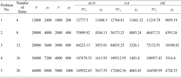
number of items (4, 8, 12, 16, and 20 items) are given in this section. The initial data of all test problems are shown in Table (1). In these examples, a unique value is assumed for both
1
and 2 as 10, 23. Moreover, in Table (2), the fuzzy data of resources with their tolerances for the five test problems are presented. The initial parameter values for implementation of ACO, GA and DE are given in Table (3). All the test problems are solved on a personal computer with Intel core i3-2100 processor having 3.10GHz CPU and 4 Gig RAM. Furthermore, all algorithms are coded using the MATLAB 7.6.0.324 software.
Insert Table (1) about here Insert Table (2) about here Insert Table (3) about here
The steps involved in the proposed procedure to solve the test problems are illustrated as follow.
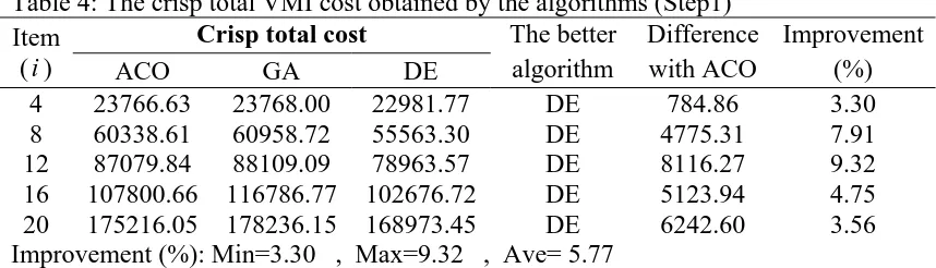
Step 1: In a given test problem, determine the total cost of all items using Eq. (14) by ACO, GA, and DE.
21
Insert Table (4) about here Insert Table (5) about here
Insert Figure (8) about here Insert Figure (9) about here Insert Figure (10) about here Insert Figure (11) about here
Step 2: Determine the total cost of all items in fuzzy model (25) using ACO, GA, and DE. To solve the fuzzy model given in (25), two minimum total cost TC0 and TC1 are first found based on what was discussed in Subsection 4.7.2 to obtain p0 (TC1TC0). The results are shown in Table (2). Then, the five fuzzy test problems modeled in (25) are solved using GA, ACO, and DE. The number of runs for these algorithms is 10, for each test problem, where their minimum fuzzy total costs of the entire SC VMI chain, the least CPU times (seconds), and values are shown in Tables (6)-(8), respectively.
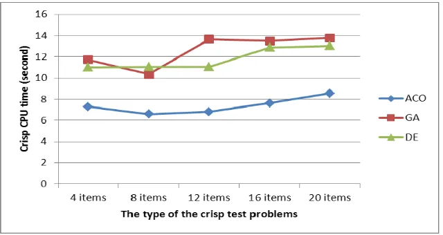
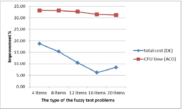
Based on the results given in Table (6), DE is completely the superior algorithm for the total cost in the fuzzy model given in (25). In contrast, based on the results in Table (7), ACO is the better algorithm for the least CPU time (seconds) in the fuzzy model. Figures (12) and (13) show this dominance better. Furthermore, in terms of fuzzy SC VMI total cost, the DE improvement percentages over ACO are 18.72, 15.29, 10.40, 6.20, and 8.41 for 4, 8, 12, 16, and 20 item problems, respectively. In addition, in terms of the CPU time, the ACO improvement percentages with respect to DE are 33.19, 33.16, 32.66, 31.48, and 31.22 seconds for 4, 8, 12, 16, and 20 item problems, respectively. Both improvement fashions are presented in Fig. 14. Consequently, DE in terms of the total cost has a slightly decreasing improvement movement from small test problem to large test problem. Similarly, CPU improvement trend by ACO has a sharp falling until 16-item test problem and after that a little rise. In terms of value, the results in Table (8) indicate that DE is the best algorithm in most of the test problems.
22
Insert Table (8) about here
Insert Figure (12) about here Insert Figure (13) about here Insert Figure (14) about here
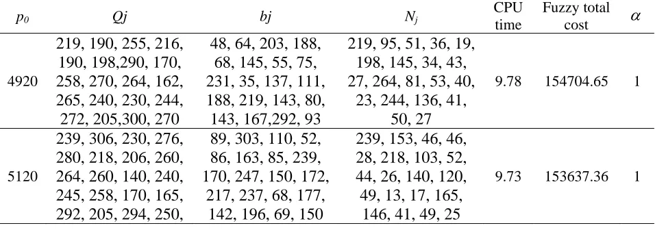
Step 3: Sensitivity analysis for tolerance of objective function (p0) by the better algorithm. In this step, we examine the effect of p0 variation on other parameters. To do this, the fuzzy model (25) is solved with different p0 for the 20-item test problem using DE.
The results are presented in Table (9). Based on the results in this Table, with 20.32% increasing p0 value, the fuzzy total cost has a gentle decline about 5.17%, while the
values remain stable. As a result, the tolerance of the objective function (p0) has an inverse relation with the fuzzy total cost. This can be a key point for SC decision makers. Similarly, Fig. 15 shows the variation of fuzzy total cost with respect to different value of p0 for the 20-items test problem.
Insert Table (9) about here
Insert Figure (15) about here
7. Conclusions and recommendation for future research
23
applicability of the proposed methodology along with a sensitivity analysis on its parameter was shown using five numerical examples in an Iranian automobile supply company containing different numbers of items. The results showed that in both the crisp and the fuzzy models, while the ant colony optimization algorithm was the best algorithm in terms of the required CPU time, differential evolution was the superior algorithm in terms of the total cost. In addition, based on the results in Table (9), the tolerance of objective function (p0) has an inverse relation with the fuzzy total cost. This can be a key point for SC decision makers.
For future researches in this area, the followings are recommended: (a) Quantity discounts can be allowed
(b) In addition to backorders, lost sales can also be assumed for shortages
(c) Other search-heuristic algorithms such as simulated annealing (SA), imperialist competitive algorithm (ICA), and particle swarm optimization (PSO) may also be employed to solve the problem
(d) Instead of EOQ, economic production quantity (EPQ) model can be considered
(e) Multi-echelon supply chain such as one-buyer multi-supplier, multi-buyer one-supplier, and multi-buyer multi-supplier supply chains can be investigated.
References
Aarts, E.H.L., Korst, J.H.M., 1989. Simulated annealing and Boltzmann machine; a stochastic approach to computing (1st ed.). Chichester, U.K: John Wiley and Sons.
Abbasi, B., Mahlooji, H., 2012. Improving response surface methodology by using artificial neural network and simulated annealing. Expert Systems with Applications, 39(3), 3461– 3468.
Alex, R., 2007. Fuzzy point estimation and its application on fuzzy supply chain analysis. Fuzzy Sets and Systems, 158(14), 1571–1587.
Alfi, A., Fateh M.-M., 2011. Intelligent identification and control using improved fuzzy particle swarm optimization. Expert Systems with Applications, 38(10), 12312–12317.
Aliev, R.A., Fazlollahi, B., Guirimov, B.G., Aliev, R.R., 2007. Fuzzy-genetic approach to aggregate production–distribution planning in supply chain management. Information Science, 177(20), 4241–4255.
24
Becerra, R.L., Coello, C.A.C., 2006. Cultured differential evolution for constrained optimization. Computer Methods in Applied Mechanics and Engineering, 195(33-36), 4303– 4322.
Cárdenas-Barrón, L.E., 2011. The derivation of EOQ/EPQ inventory models with two backorders costs using analytic geometry and algebra. Applied Mathematical Modelling, 35(5), 2394–2407.
Cárdenas-Barrón, L.E., Treviño-Garza, G., Wee, H.M., 2012. A simple and better algorithm to solve the vendor managed inventory control system of multi-product multi-constraint economic order quantity model. Expert Systems with Applications, 39(3), 3888–3895.
Chen, H., Chen, J., Chen, Y., 2006. A coordination mechanism for a supply chain with demand information updating. International Journal of Production Economics, 103(1), 347– 361.
Colorni, A., Dorigo, M., Maniezzo, V., 1991. Distributed optimization by ant colonies, in: Proceedings of European Conference on Artificial Life, Paris, France, 134–142.
Colorni, A., Dorigo, M., Maniezzo, V., 1992. An investigation of some properties of an ‘‘ant algorithm’’, in: Proceedings of the Parallel Problem Solving from Nature Conference, Brussels, Belgium, 509–520.
Colorni, A., Dorigo, M., Maniezzo, V., 1994. Ant system for job-shop scheduling, Belgian Journal of Operations Research, Statistics and Computer Science, 34(1) 39–53.
Darwish, M.A., Odah, O.M., 2010. Vendor managed inventory model for single-vendor multi-retailer supply chains. European Journal of Operational Research, 204(3), 473–484. Danese, P., 2006. The extended VMI for coordinating the whole supply network. Journal of Manufacturing Technology Management, 17(7), 888–907.
Dong Y., Xu, K., 2002. A supply chain model of vendor managed inventory. Transportation Research Part E, 38(2), 75–95.
Dorigo M., Stutzle T., 2004. Ant colony optimization. Cambridge, MA, USA: MIT Press. Dorling, K., 2006. Determinants of successful vendor managed inventory relationships in oligopoly industries. International Journal of Physical Distribution and Logistics Management, 36 (3), 176–191.
Dueck G., Scheuer T., 1990. Threshold accepting: A general purpose algorithm appearing superior to simulated annealing. Journal of Computational Physics, 90(1), 161–175.
25
Gen M., Cheng R., 1997. Genetic algorithm and engineering design (1st ed.). New York, NY, U.S.A: John Wiley & Sons.
Hadley, G., Whitin, T. M., 1963. Inventory systems. Prentice Hall
Harris, F.W., 1913. How many parts to make at once, Factory, The Magazine of Management 10 (2), 135-136, & 152.
Hosseini, S.V., Moghadasi, H., Noori, A.H., Royani, M.B., 2009. Newsboy problem with two objectives, fuzzy costs and total discount strategy. Journal of Applied Sciences, 9(10), 1880– 1888.
Huang, F.Z., Wang, L., He, Q., 2007. An effective co-evolutionary differential evolution for constrained optimization. Applied Mathematics and Computation, 186(1), 340–356.
Jaberipour, M., Khorram, E., 2011. A new harmony search algorithm for solving mixed-discrete engineering optimization problems. Engineering Optimization, 43(5), 507–523. Joo, S.J., Bong, J.Y., 1996. Construction of exact D-optimal designs by Tabu search. Computational Statistic and Data Analysis, 21(2), 181–191.
Kaveh, A., Ahangaran, M., 2012. Discrete cost optimization of composite floor system using social harmony search model. Applied Soft Computing Journal, 12(1), 372-381.
Kaveh, A., Laknejadi, K., 2011. A novel hybrid charge system search and particle swarm optimization method for multi-objective optimization. Expert Systems with Applications, 38(12), 15475–15488.
Kristianto, Y., Helo, P., Jiao, J.(R.), Sandhu, M., 2012. Adaptive fuzzy vendor managed inventory control for mitigating the Bullwhip effect in supply chains. European Journal of Operational Research, 216(2), 346–355
Laumanns, M., Thiele, L., Deb, K., Zitzler, E., 2002. Combining convergence and diversity in evolutionary multi-objective optimization. Evolutionary Computation, 10(3), 263–282. Lee, K.M., Hsu, M.R., Chou, J.H., Guo, C.Y., 2011. Improved differential evolution approach for optimization of surface grinding process. Expert Systems with Applications, 38(5), 5680–5686.
Liao, T.W., 2010. Two hybrid differential evolution algorithms for engineering design optimization. Applied Soft Computing, 10(4), 1188–1199.
26
Liu, H., Cai, Z., Wang, Y., 2010. Hybridizing particle swarm optimization with differential evolution for constrained numerical and engineering optimization. Applied Soft Computing, 10(2), 629–640.
Mondal, S., Maiti, M., 2002. Multi-item fuzzy EOQ models using genetic algorithm. Computers & Industrial Engineering 44(1), 105–117.
Pasandideh, S.H.R., Niaki, S.T.A., Nia, A.R., 2010. An investigation of vendor-managed inventory application in supply chain: the EOQ model with shortage. International Journal of Advanced Manufacturing Technology, 49(1-4), 329–339.
Pasandideh, S.H.R., Niaki, S.T.A., Nia, A.R., 2011. A genetic algorithm for vendor managed inventory control system of multi-product multi-constraint economic order quantity model. Expert Systems with Applications, 38(3), 2708–2716.
Petrovic, D., Roy, R., Petrovic, R., 1998. Modelling and simulation of a supply chain in an uncertain environment. European Journal of Operational Research, 109(2), 299–309.
Petrovic, D., Roy, R., Petrovic, R., 1999. Supply chain modelling using fuzzy sets. International Journal of Production Economics, 59(1-3), 443–453
Petrovic, D., 2001. Simulation of supply chain behaviour and performance in an uncertain environment. International Journal of Production Economics, 71(1-3), 429–438.
Pohlen, T., Goldspy, T., 2003. VMI and SMI programs: How economic value added can help sell the change. International Journal of Physical Distribution and Logistics Management, 33(7), 565–581.
Razemi, J., Rad, R.H., Sangari, M.S., 2010. Developing a two-echelon mathematical model for a vendor-managed inventory (VMI) system. International Journal of Advanced Manufacturing Technology, 48(5-8), 773–783.
Schmid, V., Doerner, K.F., Laporte, G., 2013. Rich routing problems arising in supply chain management. European Journal of Operational Research, 224(3), 435–448
Selim, H., Araz, C., Ozkarahan, I., 2008. Collaborative production–distribution planning in supply chain: A fuzzy goal programming approach. Transportation Research Part E, 44(3), 396–419.
Shah, J., Goh, M., 2006. Setting operating policies for supply hubs. International Journal of Production Economics, 100(2), 239–252.
27
Stapleton, D., Hanna, J., Ross, R., 2006. Enhancing supply chain solutions with the application of chaos theory. Supply Chain Management: An international Journal, 11(2), 108–114.
Storn, R., Price, K.V., 1997. Differential evolution: a simple and efficient heuristic for global optimization over continuous spaces. Journal of Global Optimization, 11(4), 341–359.
Taft, E.W., 1918. The most economical production lot. Iron Age, 101, 1410–1412.
Taleizadeh, A.A., Aryanezhad, M.B., Niaki, S.T.A., 2008. Optimizing multiproduct multi-constraint inventory control systems with stochastic replenishment. Journal of Applied Sciences, 8(7), 1228–1234.
Taleizadeh, A.A., Niaki, S.T.A., Hosseini, V., 2009. Optimizing product multi-constraint bi-objective newsboy problem with discount by a hybrid method of goal programming and genetic algorithm. Engineering Optimization, 41(5), 437–457.
Taleizadeh, A.A., Niaki, S.T.A, Shafii, N., Ghavamizadeh Meibodi, R., Jabbarzadeh A., 2010. A particle swarm optimization approach for constraint joint single buyer single vendor inventory problem with changeable lead-time and (r,Q) policy in supply chain. International Journal of Advanced Manufacturing Technology, 51(9-12), 1209–1223.
Taleizadeh, A.A., Niaki, S.T.A., Makui, A., 2012. Multiproduct multiple-buyer single-vendor supply chain problem with stochastic demand, variable lead-time, and multi-chance constraint. Expert Systems with Applications, 39(5), 5338–5348.
Thomas, D.J., Griffin, P.M., 1996. Coordinated supply chain management. European Journal of Operational Research, 94(1), 1–15.
Wang, J., Shu, Y.F., 2005. Fuzzy decision modeling for supply chain management. Fuzzy Sets and systems, 150(1), 107–127.
Xie Y., Petrovic D., Burnham, K., 2006. A heuristic procedure for the two-level control of serial supply chains under fuzzy customer demand. International Journal of Production Economics, 102(1), 37–50.
Yager, R., 1979. Ranking fuzzy subsets over the unit interval, in: Proceedings of 17th IEEE International Conference on Decision and Control, San Diego, CA, 1435–1437.
Yager, R., 1981. A procedure for ordering fuzzy subsets of the unit interval. Information Sciences, 24(2), 143–161.
28
Yu, Y., Wang, Z., Liang, L., 2012. A vendor managed inventory supply chain with deteriorating raw materials and products. International Journal of Production Economics, 136(2), 266–274.
Zimmermann, H.J., 1976. Description and optimization of fuzzy system. International Journal of General Systems, 2(4), 209–215.
29
Figure (1): An illustration of a traditional supply chain
Figure (2): Triangular fuzzy number
Figure (3): Fuzzy resource with tolerance pi
R c L
c c
c
1
c R
d c c
c L
d c c
i
b
1
i
30
Figure (4): Basic Ant Colony Optimization behavior at different time stamps. The green areas represent the amount of pheromones on each path
Initialize (set parameters) repeat
Each ant is located on the primary node repeat
Each ant employs a state move rule to increase the solution
Apply the pheromone local update rule
until all the ants have made a complete solution Apply a local search method
Apply the pheromone global update rule until the stop conditions is fulfilled
31
Figure (6): Flowchart of the solving procedure Propose the VMI of
item multi-constraint EOQ SC model under shortage
Analysis and comparing the crisp
results from three algorithms
Considering fuzzy environment to convert the crisp
problem
Defuzzification of the model by two
methods
Solving the crisp problem by DE Solving the crisp
problem by GA Solving the crisp
problem by ACO
Analysis and comparing the results from three
algorithms
Solving the problem by DE Solving the problem
by GA Solving the problem
by ACO
32
Figure (7): The representation of the solution for the test problem with 10-item
Figure (8): The crisp total cost comparison of meta-heuristic algorithms (step1)
33
Figure (10): DE and ACO improvement trends for total cost and CPU time respectively (step1)
Figure (11): The graph of the minimum total cost using DE for the 20-item crisp problem (step 1)
34
Figure (13): The fuzzy CPU time comparison of meta-heuristic algorithms (step2)
Figure (14): DE and ACO improvement trends for fuzzy total cost and CPU time respectively (step2)
Figure (15): The variation of fuzzy total cost with respect to different values of p0 for the
36 Table 2: Data of problem resources
Problem No.
Number of Items
F p1 V p2
ACO GA DE
0
TC p 0 TC 0 p 0 TC 0 p 0
1 4 12000 2400 1000 200 12777.5 11048.5 12784.81 11041.32 11219.78 9059.19
2 8 20000 4000 2000 400 55809.92 4544.13 56373.23 4083.24 46437.21 4393.26
3 12 28000 5600 3000 600 84223.13 3055.01 84835.25 3226.1 72132.91 10108.82
4 16 36000 7200 4000 800 107678.53 1613.93 109512.95 1483.4 100957.43 1914.4
5 20 44000 8800 5000 1000 169922.65 5637.55 172602.56 4063.43 164589.99 4720.53
Table 3: The initial parameter values for ACO, GA, and DE
DE GA
ACO
NP=300 Probability of crossover (Pc)=0.8
Number of ant=200
F Factor =0.05 Probability of mutation (PM)=0.05
Rate of evaporation=0.2
CR Factor =0.4 Probability of reproduction (PE)=0.15
Population(NGA)=200
Stopping criterion=200 iterations Stopping criterion=200 iterations
37 Table 4: The crisp total VMI cost obtained by the algorithms (Step1) Item
( i )
Crisp total cost The better algorithm
8 60338.61 60958.72 55563.30 DE 4775.31 7.91
12 87079.84 88109.09 78963.57 DE 8116.27 9.32
16 107800.66 116786.77 102676.72 DE 5123.94 4.75 20 175216.05 178236.15 168973.45 DE 6242.60 3.56 Improvement (%): Min=3.30 , Max=9.32 , Ave= 5.77
Table 5: The required CPU time of the algorithms (Step1) Item
( i )
Crisp CPU time (seconds) The better algorithm
Table 6: The fuzzy total VMI cost obtained by the algorithms (Step2) Item
( i )
Fuzzy total cost The better algorithm
4 19320.20 19320.20 15703.45 DE 3616.75 18.72
8 56207.59 57058.55 47614.81 DE 8592.78 15.29
12 85671.46 86926.37 76763.63 DE 8907.83 10.40
38
Table 7: The required CPU times of the algorithms to solve the fuzzy VMI (Step2) Item
( i )
Fuzzy CPU time (seconds) The better algorithm Table 8: The fuzzy -values obtained by the algorithms (Step2) Item
Table 9: Effect of variation of p0 for the fuzzy test problem with 20-items