Nonlinear dependencies on Brazilian equity
network from mutual information minimum
spanning trees
A. Q. Barbi, G. A. Prataviera
Departamento de Administra¸c˜ao, FEA-RP, Universidade de S˜ao Paulo, 14040-905, Ribeir˜ao Preto, SP, Brazil
Abstract
Mutual information minimum spanning trees are used to explore nonlinear de-pendencies on Brazilian equity network in the periods from June 2015 to January 2016 and from January 2016 to September 2016, corresponding to the government transition from President Dilma Rousseff to the current President Michel Temer, respectively. Minimum spanning trees from mutual information and linear corre-lation between stocks returns were obtained and compared. Mutual information minimum spanning trees present higher degree of robustness and evidence of power law tail in the weighted degree distribution, indicating more risk in terms of volatility transmission than it is expected by the analysis based on linear cor-relation. In particular, a remarkable increase of stock returns nonlinear depen-dencies indicates that Michel Temer’s period is more risky in terms of volatility transmission network structure. Also, we found evidence of network structure and stock performance relationship.
Keywords: Stock market network, Emerging markets, Mutual information, Nonlinear dependence, Minimum spanning tree.
1. Introduction
Financial Markets are complex systems whose structure and behav-ior are strongly dependent on their components interrelations. In partic-ular, network theory has contributed to characterize and understand the
Email addresses:[email protected](A. Q. Barbi),[email protected](G. A. Prataviera)
behavior of financial markets. Previous studies indicate that market net-work structure may contain useful information to characterize and even to predict the market behavior such as the occurrence of a financial crisis. An interesting method to analyze such structures started with the seminal work of Ref. [1] using minimum spanning trees (MST). The MST is par-ticularly suitable for extracting the most important information when a large number of linkages is under consideration. However, most of these studies are based on linear dependencies given by Pearson’s linear cor-relation coefficient [2–7]. Thus, it is important to introduce measures of nonlinear dependence between components of a network. In particular, mutual information is a promising alternative to Pearson’s coefficient as a measure of nonlinear dependence [8–10]. Actually, the combination of information theory and network analysis has already proved useful for research on financial markets [11–13]. Moreover, few studies [14] system-atically compares the networks generated through Pearson’s correlation with those generated through mutual information.
The Brazilian equity market is one of the most important in Latin Amer-ica and of emerging markets. It has a signifAmer-icant number of worldwide big companies, like Ita ´u Bank (42nd), Bradesco Bank (67th), Vale do Rio Doce (2nd mining company) and Petrobr´as (13rd oil & gas company), according to the latest Forbes ranking. Additionally, Brazil is currently the 9th largest economy in the world, according to International Monetary Fund. How-ever, the country has been the target of a series of corruption and money laundering investigations, notably the largest operation of this kind in the world, the so called ”Lava Jato” (Car Wash) operation. This political tur-moil has brought great volatility to financial market in recent years, even more after President Dilma Rousseff’s impeachment event in 2016. Inside this mess, the current president Michel Temer took on. Thus, understand-ing the economic and political role in the financial network is important. Concerning the Brazilian market, the few network-based studies are re-stricted to MST based on linear dependencies using Pearson’s correlation coefficient [4,15]. So, we consider important to extend this kind of analysis taking into account asset’s nonlinear interactions.
periods because they are very dissimilar even during a short time win-dow. While during Rousseff’s period, stocks values went down more than 40%, just six months after government transition, stocks valued up around 50%. We investigated such turbulence analyzing networks structures ob-tained from Bovespa’s high frequency stock returns. Our results suggest that the networks obtained from mutual information present a more inter-connected overall dependence, with stronger volatility transmission struc-ture, notably during Michel Temer’s period. Finally, the analysis of the network in the financial market via mutual information brings benefits to the investment decision making, particularly with regard to the analysis of the network structure and stock’s performance.
The article is organized as follows: in Section (2) we discuss the method-ology to obtain and analyze mutual information minimum spanning trees. In Sec.(3) we present the data, and Sec. (4) shows the results by contrasting the networks obtained from mutual information with those obtained with Pearson’s linear correlation. Finally, in (5) we present the conclusion.
2. Methodology
2.1. Nonlinear dependence and Minimum Spanning Tree
Here we are interested in analyze dependencies between stock price returns. The return of a given asset at timetis defined by
ri(t) =ln pendence between assets we use a parameter based on mutual informa-tion. The mutual information between two stock returns ri and rj with
joint probability density f(ri,rj)is defined as [16,17]
well known that statistical independence imply the vanishing of Pearson’s correlation coefficientρi,jdefined by
ρij = q hrirji − hriihrji
(hr2ii − hrii)2(hr2
ji − hrji)2
, (3)
which is easily estimated from empirical data, and where h.i stands for statistical mean. However, the vanishing of correlation does not in general imply thatriandrjare independent. Therefore, MI is a more general
mea-sure of dependence that goes beyond the usual linear relationship given by Pearson’s correlation.
On the other hand, Pearson’s correlation and MI are not directly com-parable since the first one varies in the interval [−1, 1] while the second one may assume values in the interval[0,∞). Then, they should be scaled
over the same range. In addition, the degree of linear dependence given by Pearson’s correlation is better associated with its absolute or its square value. In this paper we use a dependence coefficient whose definition is based on the fact that the MI for a bivariate normal density is given by [17]
Iij =−1
2ln
1−ρ2ij. (4)
Eq. (4) shows that correlation implies dependence for a bivariate normal distribution . Now, the inversion of Eq. (4) allows to define the following global coefficient of dependence [11,18]
λij =
q
1−e−2Iij, (5)
which is limited to the interval[0, 1], and can be compared with the linear correlation absolute value. In addition, a value of λij > ρij ≈ 0 indicates
nonlinear dependence.
With the global dependence coefficient we can define a distance func-tion
dij(global) = 1−λij, (6)
which can be directly compared with a distance based on Pearson’s corre-lation coefficient
The distances defined by Eqs. (6) and (7) will be used to obtain the network minimum spanning tree (MST). The MST is a simply connected graph that connects all Nnodes with N−1 edges such that the sum of all edge dis-tances is a minimum, thus reducing the information contained in N(N−
1)/2 dependence coefficients to(N−1)edges. Kruskal’s algorithm [19] is one of the main algorithms for searching a MST. It adds new weaker links until there are no new additions without making a cycle. This process finishes when the graph is fully connected.
Furthermore, to obtain the MI and the coefficient of dependence in Eq. 5, we need to estimate the empirical density functions f(ri,rj), f(ri), and
f(rj)from data. Here we use the non-parametric method of kernel density estimation [20–22]. For ad-dimensional set of variables x = (r1,· · · ,rd)T
and the given data set {r1,· · · ,rn} whose density is to be estimate, the
multivariate kernel density estimator with kernel K and window widths h1,· · · ,hdis defined as
where the kernel function satisfies R
dK(x)dx = 1. In this work we use
the Gaussian kernel, which for a radially symmetric standard multivariate normal distribution is written as
K(x) = e
−1 2xTx
(2π)d/2. (9)
Besides, for the window bandwidth we use the criteria that minimizes the density mean integrated square error and whose optimal value for a multivariate Gaussian kernel is given by [21,22]
hi =
where ˆσi is the sample standard deviation of variable i, and d = 2 for a bivariate kernel.
2.2. Network measures
networks where hubs are much more connected then what is expected by Poisson distribution of random networks. This lack of scale can be analyzed by the scaling parameter α of a power law distribution, whose calculation is given by the maximum likelihood estimator [23]
α =1+n parameter that can be estimated using Kolmogorov-Smirnov statistic [24]. For this purpose, the R poweRlaw package [25] is employed. Since we are interested in the strength of the dependencies, we use the weighted degree distribution in our analysis. This means that a given degree will be weighted by the values ofλij or|ρij|.
To estimate network’s financial systemic risk, we can determine its ro-bustness coefficient, given by [23]
R=1− 1
hk2i
hki −1
, (12)
where hki andhk2i are the degree distribution first and second moments, respectively. The robustness coefficient represents the fraction of nodes in a network that we need to remove to lose its component structure. Here, we use this metric to evaluate the network’s concentration structure. The bigger the nodes that are very highly connected (a hub), the higher the network’s robustness coefficient, until it approximates to 1.
In order to measure hubs strength individually, we use the node’s eigen-vector centrality. This parameter indicates that a node is important if it is connected to other nodes that are also important. So, the centrality xi of vertexiis defined by [26]
xi =κ1−1
∑
j
Aijxj, (13)
where for us Aij = λij (or |ρij|) are the entries of the MST weighted
adja-cency matrix A,κ1is the largest eigenvalue of A, andxjis the centrality of
Those measures are useful to identify volatility transmission in finan-cial networks. Volatility transmission means that once a hub gets affected by certain volatility, it spreads that instability through its connections, pos-sibly causing a financial instability. This same logic can be used for a vari-ety of systems, like the power grid network. For example, on August 10, 1996, Oregon, a line carrying 1,300 megawatts sagged close to a tree and snapped, while its current was automatically shifted to two lower-voltage lines. However, these too failed. This day, a full blackout happened in 11 US states. In this example, that line (a hub) had a significant energy that could not be tolerated by the other nodes if it fails, possibly causing a cascade effect. In financial networks, an important asset (hub) can also be affected by a certain volatility, such as a news about an accounting fraud in a big bank. Then, quickly many others might feel the impact of the news, especially if they have with it a strong dependence. Thus, a high value of robustness coefficient means that the network has a strong interconnected structure, that is, a significant overall dependence among assets. More, that it has a very significant hub. In this way, there’s more probability that a great turmoil affects more and more stocks, like in a domino effect [27].
3. Data
The data set for this paper comes from the Bovespa Index (Ibovespa), which comprises a portfolio of the main Brazilian assets, and is the most important index of average performance for the Brazilian stock market prices. The share of each stock in the Ibovespa portfolio is directly related to its representativeness in terms of the number of trades and financial volume. This is given by the Stock Negotiability Index (SNI)
SN I =
r
ni
N ×
vi
V, (14)
where ni is the number of deals with the stock i, N is the total number of trades, vi is the financial volume generated by the trades with the i
Our analysis is restricted to data from two periods that we consider relevant. The first period, from 06/01/2015 to 01/26/2016, was under the government of President Dilma Rousseff, with 159 trading sessions and index return of -42%, where we collected 3888 stock returns, given every 15 minutes. The second one, a period from 01/27/2016 to 09/08/2016, un-der the government of President Michel Temer, with 160 trading sessions and index return of 50%, where we obtained 3969 returns, given every 15 minutes. Data were collected from Bovespa ftp site [29]. It contains high frequency trading data for various Brazilian financial instruments. For this purpose, we used the GetHFData package from R software [30].
All statistical and network analysis obtained in this paper were carried out inRsoftware, while Gephi was useful for network illustration design.
4. Results and discussion
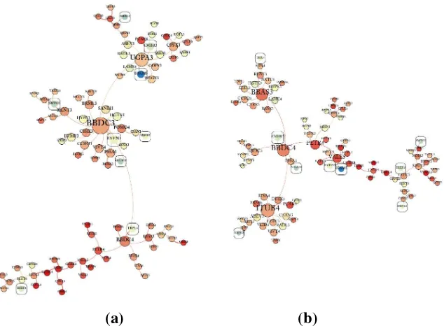
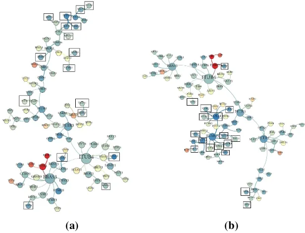
Fig. 1a-b shows the MST network structure for the Dilma Rousseff’s (DR) period, obtained from the distances based on linear and global de-pendence, respectively. To identify individual differences, we highlighted into a square, stocks which may make up the portfolio that maximizes the so-called Sharpe index, through the efficient frontier selection technique [31]. This index selects portfolios with the best return-risk ratio. Fig. 2 a-b shows the same as in Fig. 1 but for Michel Temer’s (MT) period. We observe that MST based on linear correlation the stocks with best Sharpe index are widespread throughout the network for both periods. For the mutual information MSTs, they are concentrated at the periphery for DR period, while they are more central for MT period. The mean distances for each network are depicted in the captions of Figs. 1and 2, which shows that the MSTs based on MI are more concentrated, most notably during MT period.
(a) (b)
Figure 1: MST for Dilma Rousseff’s period. (a) MST based on linear correlation; (b) MST based on mutual information. Nodes size is related to eigenvector centrality, and color hue degree to the stock variation in the period, red for negative returns, until dark blue, for positive ones. Stocks are highlighted into a square if it composes a minimum of 3% of the portfolio that maximizes the Sharpe index. MST mean distance: (a) 0.64; (b) 0.56.
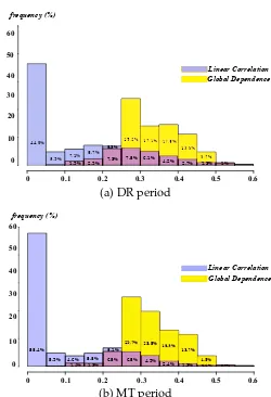
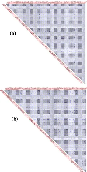
we show a pictorial representation of the symmetric matrix whose entries are given by the absolute value difference between the global dependence coefficient and linear correlation for both periods, and whose entries are represented by color intensity, so that dark points corresponds to a dif-ference of at least 0.3. The higher concentration of dark points in Fig. 4b shows that this period is characterized by an increasing asset’s nonlinear dependence. In fact, the linear correlation structure in MT period has a lower overall dependence than in DR period, as shown in Fig. 3. This indicates that a risk analysis based on linear correlation for MT period is even less appropriate.
(a) (b)
Figure 2: MST for Michel Temer’s period. (a) MST based on linear correlation; (b) MST based on mutual information. Stocks are highlighted into a square if it composes a min-imum of 3% of the portfolio that maximizes the Sharpe index. MST mean distance: (a) 0.66; (b) 0.54.
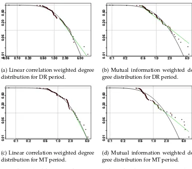
include a log-normal density fitting (black line). By comparing Figs. 5a-5c with5b-5d, we see that the weighted degree distribution for linear correla-tion MSTs follows more closely the log-normal distribucorrela-tion, while for the mutual information MSTs the tail dependence is close to a power law. The power law tail is even more evident in Fig. 5d, which corresponds to the period with more nonlinear dependencies. This tail behavior allows that we find nodes with very high degree values with a higher probability.
In Table1, the assets were splitted into two groups, (a) containing the mean returns of the 20 assets with the highest and lowest eigenvector cen-trality, and (b) the mean weighted degree of the 20 stocks with the highest and lowest returns for the networks based on linear correlation and global dependence, and whereµrandσrstands for mean and standard deviation
of returns, andµkandσkare the mean and standard deviation of weighted
Histograma R vs. IM
(a)
(b)
Figure 4: Pictorial representation of the symmetric matrix whose entries are given by
|λij− |ρij||. (a) Dilma Rousseff’s period; (b) Michel Temer’s period. Dark dots show
0.05 0.10 0.200.01 0.50 1.00 2.00 5.00
(a) Linear correlation weighted degree distribution for DR period.
(b) Mutual information weighted de-gree distribution for DR period.
0.1 0.2 0.5 1.0 2.0 5.0
(c) Linear correlation weighted degree distribution for MT period.
(d) Mutual information weighted de-gree distribution for MT period.
Figure 5: Weighted degree complementary cumulative distribution function for each pe-riod in a log-log scale. The power law fitting is depicted by the green line. Estimated scaling parameter: (a)α= 3.03; (b)α= 2.44; (c)α= 4.19; (d)α= 2.39. The lognormal density fit in black line was included for comparative purposes.
centrality and assets returns. For example, as shown in Table 1(a), if an investor, using the information of networks based on mutual information, put his money on the 20 assets with the largest centralities, during the MT period he would have gained 40% more than if he had only used an analysis based on linear correlation networks. Furthermore, for the DR period, if the investor uses the information of networks based on mutual information, he would also have saved almost 20% of loss, providing that he knows the strategy of investing in less central assets. In fact, in Table 1(b), we see that, in the MT period, the best assets returns are related to the highest weighted degree, and to the smallest in the DR period.
Table 1: Relationship between centrality and stock returns. (a) Mean returns of the 20 stocks with the highest and lowest eigenvector centrality; (b) weighted degree of the 20 stocks with the highest and lowest returns. µr and σr stands for mean and standard
deviation of returns, and µk andσk are the mean and standard deviation of weighted
degree.
Period Dilma Rousseff Michel Temer
(a) Returns of the 20 stocks with the highest and lowest eigenvector centralities
more central less central more central less central
µr σr µr σr µr σr µr σr
Linear correlation -20.4% 14.7% -27.7% 33.1% 64.3% 63.3% 64.4% 67.9%
Global dependence -32.7% 19.1% -8.3% 24.9% 105.5% 126.7% 46.5% 63.8%
(b) Weighted degree of the 20 stocks with the highest and lowest returns
best returns worst returns best returns worst returns
µk σk µk σk µk σk µk σk
Linear correlation 1.45 0.83 1.90 1.21 2.2 1.4 1.5 0.76
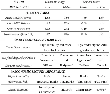
Table2shows the main results of this work. Part (a) of Table 2shows some network metrics. We see that for mutual information networks, the mean MST distance has declined 18% for period MT and just 12.5% for pe-riod DR. Despite the mean degree remains the same, the robustness coef-ficient, calculated from Equation (12), increases by 27% during period MT (during DR, it raises 5%), while power law α parameter, calculated from Equation (11), decreases from 4.19 to 2.39 during period MT (for period DR it decreased from 3.03 to 2.44), which is a significant change.
The part (b) of Table2shows some MSTs qualitative features. As seen in Table 1(b), both linear correlation and mutual information spanning trees suggests that stock returns are related to their centralities, but this is much more evident for networks based on mutual information. In addi-tion, in the linear correlation networks all the best Sharpe index assets are diffuse around the tree. On the other hand, in the mutual information net-works, for DR period, the assets with the greatest Sharpe indices appears on the periphery of the graph, while for MT period these same stocks are now much more central. In fact, for DR period, the most central assets ’moved’ the market to a 42% negative return, whereas assets with the best Sharpe index remains into the periphery. During MT period, central assets now push the market to a 50% positive return. In this period, Sharpe’s best indices remain on the central part of the graph. These results suggests that the central stocks are the ones that really ’move’ the market.
Table 2: Paper main results
PERIOD Dilma Rousseff Michel Temer
DEPENDENCE Linear Global Linear Global
(a) MST METRICS
Mean weighted degree 1.98 1.98 1.99 1.99
Mean MST distance 0.64 0.56 0.66 0.54
Scale parameter (α) 3.03 2.44 4.19 2.39
Robustness coefficient (R) 0.62 0.65 0.56 0.71
(b) MST MAIN CHARACTERISTICS
Centrality vs. returns High centrality indicates bad stock returns
High centrality indicates
good stock returns
Weighted degree distribution Closer to a log-normal
Sharpe index dispersion Diffuse Peripheral Diffuse Central
(c) ECONOMIC SECTORS IMPORTANCE
evidence in the mutual information minimum spanning trees weighted degree distributions. Finally, mutual information network analysis seems to bring benefits to the investment decision making process, particularly concerning the analysis of network structure and stock performance. More-over, those type of networks seems to be useful to identify risk not cap-tured by a linear correlation network analysis. For further research it would be interesting to replicate this kind of study for other developing countries or to diverse types of markets, such as currencies.
Lastly, network analysis is a rapidly developing science, and it would not be surprising if we have much faster, more flexible and interactive methods of data analysis and visualization in a short time. For us, by now it is enough to think that if the key determinant for estimating financial risk models is the dependency structure among all its assets, it seems that having an accurate map at hand is already a great starting point.
6. Acknowledgements
The authors gratefully acknowledge financial support from the Brazil-ian agency CNPq.
References
References
[1] R. Mantegna,Hierarchical structure in financial markets, Eur. Phys. J. B 11 (1) (1999) 193–197. doi:10.1007/s100510050929.
URLhttp://link.springer.com/10.1007/s100510050929
[2] S. Miccich, G. Bonanno, F. Lillo, R. N. Mantegna, Degree stability
of a minimum spanning tree of price return and volatility, Physica
A: Statistical Mechanics and its Applications 324 (1-2) (2003) 66–73.
doi:10.1016/S0378-4371(03)00002-5.
URL http://linkinghub.elsevier.com/retrieve/pii/ S0378437103000025
[3] R. Coelho, C. G. Gilmore, B. Lucey, P. Richmond, S. Hut-zler, The evolution of interdependence in world equity
mar-kets: evidence from minimum spanning trees, Physica A:
doi:10.1016/j.physa.2006.10.045.
URL http://linkinghub.elsevier.com/retrieve/pii/ S0378437106010624
[4] B. M. Tabak, T. R. Serra, D. O. Cajueiro, Topological properties
of stock market networks: The case of brazil, Physica A:
Statis-tical Mechanics and its Applications 389 (16) (2010) 3240–3249.
doi:10.1016/j.physa.2010.04.002.
URL http://linkinghub.elsevier.com/retrieve/pii/ S0378437110002992
[5] C. G. Gilmore, B. M. Lucey, M. W. Boscia, Comovements in
govern-ment bond markets: A minimum spanning tree analysis, Physica A:
Statistical Mechanics and its Applications 389 (21) (2010) 4875–4886.
doi:10.1016/j.physa.2010.06.057.
URL http://linkinghub.elsevier.com/retrieve/pii/ S0378437110006059
[6] Y. Zhang, G. H. T. Lee, J. C. Wong, J. L. Kok, M. Prusty, S. A. Cheong,
Will the us economy recover in 2010? a minimal spanning tree study,
Physica A: Statistical Mechanics and its Applications 390 (11) (2011) 2020–2050. doi:10.1016/j.physa.2011.01.020.
URL http://linkinghub.elsevier.com/retrieve/pii/ S0378437111000847
[7] R. H. Heiberger, Stock network stability in times of crisis, Physica A: Statistical Mechanics and its Applications 393 (2014) 376–381.
doi:10.1016/j.physa.2013.08.053.
URL http://linkinghub.elsevier.com/retrieve/pii/ S0378437113008030
[8] A. Fraser, H. Swinney,Independent coordinates for strange attractors
from mutual information., Phys Rev A Gen Phys 33 (2) (1986) 1134–
1140.
URLhttp://www.ncbi.nlm.nih.gov/pubmed/9896728
[9] A. Kraskov, H. Stgbauer, P. Grassberger, Estimating mutual
infor-mation., Phys Rev E Stat Nonlin Soft Matter Phys 69 (6 Pt 2) (2004)
066138. doi:10.1103/PhysRevE.69.066138.
[10] J. B. Kinney, G. S. Atwal, Equitability, mutual information, and the
maximal information coefficient., Proc Natl Acad Sci U S A 111 (9)
(2014) 3354–3359. doi:10.1073/pnas.1309933111. URLhttp://dx.doi.org/10.1073/pnas.1309933111
[11] A. Dionisio, R. Menezes, D. A. Mendes, Mutual information: a
measure of dependency for nonlinear time series, Physica A:
Sta-tistical Mechanics and its Applications 344 (1-2) (2004) 326–329.
doi:10.1016/j.physa.2004.06.144.
URL http://linkinghub.elsevier.com/retrieve/pii/ S0378437104009598
[12] C. Yang, X. Zhu, Q. Li, Y. Chen, Q. Deng, Research on the evolution
of stock correlation based on maximal spanning trees, Physica
A: Statistical Mechanics and its Applications 415 (2014) 1–18.
doi:10.1016/j.physa.2014.07.069.
URL http://linkinghub.elsevier.com/retrieve/pii/ S0378437114006554
[13] P. Fiedor, Networks in financial markets based on the mutual
infor-mation rate., Phys Rev E Stat Nonlin Soft Matter Phys 89 (5) (2014)
052801. doi:10.1103/PhysRevE.89.052801.
URLhttp://dx.doi.org/10.1103/PhysRevE.89.052801
[14] H. Kaya, Eccentricity in asset management, Journal of Network The-ory in Finance 1 (2015) 1–31.
[15] B. M. Tabak, T. R. Serra, D. O. Cajueiro, The expectation hypothesis
of interest rates and network theory: The case of brazil, Physica A:
Statistical Mechanics and its Applications 388 (7) (2009) 1137–1149.
doi:10.1016/j.physa.2008.12.036.
URL http://linkinghub.elsevier.com/retrieve/pii/ S0378437108010297
[16] C. E. Shannon, A mathematical theory of
communica-tion, Bell System Technical Journal 27 (4) (1948) 623–656.
doi:10.1002/j.1538-7305.1948.tb00917.x.
[17] T. M. Cover, J. A. Thomas,Elements of Information Theory, John Wi-ley & Sons, Inc., Hoboken, NJ, USA, 2005. doi:10.1002/047174882X. URLhttp://doi.wiley.com/10.1002/047174882X
[18] H. Joe, Relative entropy measures of multivariate dependence, J Am Stat Assoc 84 (405) (1989) 157–164.
[19] J. B. Kruskal, On the shortest spanning subtree of a graph and the
traveling salesman problem, Proc. Amer. Math. Soc. 7 (1) (1956)
48–48. doi:10.1090/S0002-9939-1956-0078686-7.
URL http://www.ams.org/jourcgi/jour-getitem?pii= S0002-9939-1956-0078686-7
[20] B. W. Silverman,Density Estimation for Statistics and Data Analysis, Springer US, Boston, MA, 1986. doi:10.1007/978-1-4899-3324-9. URLhttp://link.springer.com/10.1007/978-1-4899-3324-9
[21] D. W. Scott, Multivariate Density Estimation: Theory, Practice, and
Visualization, Wiley Series in Probability and Statistics, John Wiley &
Sons, Inc, Hoboken, NJ, 2015. doi:10.1002/9781118575574. URLhttp://doi.wiley.com/10.1002/9781118575574
[22] Y. Moon, B. Rajagopalan, U. Lall, Estimation of mutual
informa-tion using kernel density estimators., Phys Rev E Stat Phys
Plas-mas Fluids Relat Interdiscip Topics 52 (3) (1995) 2318–2321. doi: 10.1103/PhysRevE.52.2318.
URLhttp://dx.doi.org/10.1103/PhysRevE.52.2318
[23] A.-L. Barabasi, Network Science, Cambridge University Press, Cam-bridge CB2 8BS, United Kingdom, 2016.
[24] A. Clauset, C. R. Shalizi, M. E. J. Newman, Power-law distributions
in empirical data, SIAM Rev. 51 (4) (2009) 661–703. doi:10.1137/
070710111.
URLhttp://epubs.siam.org/doi/abs/10.1137/070710111
[25] C. S. Gillespie, Fitting heavy tailed distributions: The poweRlaw
package, Journal of Statistical Software 64 (2) (2015) 1–16.
[26] M. Newman, Networks, Oxford University Press, 2010.
doi:10.1093/acprof:oso/9780199206650.001.0001.
URL http://www.oxfordscholarship.com/view/10.1093/acprof: oso/9780199206650.001.0001/acprof-9780199206650
[27] I. Dobson, B. A. Carreras, V. E. Lynch, D. E. Newman, Complex sys-tems analysis of series of blackouts: cascading failure, critical points,
and self-organization., Chaos 17 (2). doi:10.1063/1.2737822.
URLhttp://dx.doi.org/10.1063/1.2737822
[28] Economatica, https://economatica.com/, [Online; accessed 02-February-2017].
[29] Bovespa, ftp://ftp.bmf.com.br/, [Online; accessed 22-October-2017].
[30] M. Perlin, R. Henrique, Gethfdata: A r package for downloading and aggregating high frequency trading data from bovespa, Available at SSRN.
[31] W. F. Sharpe, Capital asset prices: A theory of market equilibrium
under conditions of risk, J Finance 19 (3) (1964) 425. doi:10.2307/
2977928.