A NEW SPECTRAL-SPATIAL FRAMEWORK FOR CLASSIFICATION OF
HYPERSPECTRAL DATA
Davood Akbaria
a
Surveying and Geomatics Engineering Department, College of Engineering, University of Zabol, Zabol, Iran - [email protected]
KEYWORDS: Hyperspectral image, Spectral-spatial classification, Support Vector Machines, Minimum Spanning Forest
ABSTRACT:
In this paper, an innovative framework, based on both spectral and spatial information, is proposed. The objective is to improve the classification of hyperspectral images for high resolution land cover mapping. The spatial information is obtained by a marker-based Minimum Spanning Forest (MSF) algorithm. A pixel-based SVM algorithm is first used to classify the image. Then, the marker- based MSF spectral-spatial algorithm is applied to improve the accuracy for classes with low accuracy. The marker-based MSF algorithm is used as a binary classifier. These two classes are the low accuracy class and the remaining classes. Finally, the SVM algorithm is trained for classes with acceptable accuracy. To evaluate the proposed approach, the Berlin hyperspectral dataset is tested. Experimental results demonstrate the superiority of the proposed method compared to the original MSF-based approach. It achieves approximately 5% higher rates in kappa coefficients of agreement, in comparison to the original MSF-based method.
1. INTRODUCTION
Imaging spectroscopy, also known as hyperspectral imaging, is concerned with the measurement, analysis, and interpretation of spectra acquired from either a given scene or a specific object at a short, medium, or long distance by a satellite sensor over the visible to infrared and sometime thermal spectral regions (Shippert, 2004). Recent technological improvements in spatial, spectral, and radiometric resolution of spectrometer imagers beget the need of developing new methods for land cover classification. A large number of researches are presented for classification of hyperspectral images (Senthil et al., 2010; Shackelford and Davis, 2003; Shrestha et al., 2005). However, they can be categorized in two major groups of the spectral or pixel-based and the spectral-spatial approaches. While the pixel- based techniques, e.g. the classic Maximum Likelihood and Support Vector Machines (SVM) classifiers, mainly emphasize the independence of pixels, the spectral-spatial approaches, e.g. Geographic Object-Based Image Analysis (GEOBIA) (Blaschke et al., 2014) and Minimum Spanning Forest (MSF) (Tarabalka et al., 2010) classifiers, employ both the spectral characteristics and the spatial context of the pixels. The importance of applying spatial patterns has been identified as a desired objective by many scientists devoted to multidimensional data analysis. These approaches have been studied from various points of views. For instance, several possibilities are discussed in (Landgrebe, 2003) for the refinement of results obtained by pixel-based techniques in multispectral imaging. This is normally done through a second step, based on a spatial context. Such contextual classification is extended also to hyperspectral images by distinguishing amongst certain land cover classes (Jimenez et al., 2005; Negri et al., 2014).
The pixel-based classification methods are often unable to accurately differentiate between some classes with high spectral similarity. This is mainly because; they take only the spectral information into account. Consequently, methods that can exploit the spatial information are crucial for producing more accurate land cover maps (Carleer and Wolff, 2006; Jensen, 2004; Shackelford and Davis, 2003). Many researchers have demonstrated that the use of spectral-spatial information improves the classification results, compared to the use of
spectral data alone, in hyperspectral imagery (Fauvel et al., 2012; Huang and Zhang, 2011; Paneque-Gálvez et al., 2013; Plaza et al., 2009; Rajadell et al., 2009; Tarabalka et al., 2011). In the early studies on spectral-spatial image classification, the spectral information from the neighborhoods are extracted by either fixed windows (Camps-Valls et al., 2006) or morphological profiles (Fauvel et al., 2008), and used to classify and label each pixel.
Segmentation techniques are the powerful tools for defining the spatial dependencies among the pixels and for finding the homogeneous regions in an image (Gonzalez and Woods, 2002). An alternative way to achieve the accurate segmentation is to perform a marker-based segmentation (Gonzalez and Woods, 2002; Soille, 2003). The idea behind this approach is to select either one or several pixels that belong to each spatial object. Each spatial object is often referred to as either a region seed, or a marker of the corresponding region. These regions, then, grow from the selected seeds. In this way, every region, in the resulting segmentation map, is associated with one region’s seed. Marker-based segmentation significantly reduces the over- segmentation and has, as a result, led to a better accuracy rate.
Tarabalka et al. have proposed an efficient approach for spectral-spatial classification using the MSF grown from automatically selected markers (Tarabalka et al., 2010). They used a pixel-wise SVM classification in order to select the most reliable classified pixels as markers. In this framework, a connected components labeling is applied on the classification map. Then, if a region is large enough, its marker is determined as the P% of pixels within this region with the highest probability estimates. Otherwise, it should lead to a marker only if it is very reliable. A potential marker is formed by pixels with estimated probability higher than a defined threshold.
In this paper, a modified spectral-spatial classification approach is proposed to improve the spectral-spatial classification of hyperspectral images. The method benefits from both MSF and SVM classifiers in an integrated framework. In the proposed approach, the SVM pixel-based algorithm is first used to classify hyperspectral images. Afterwards, for classes with low The International Archives of the Photogrammetry, Remote Sensing and Spatial Information Sciences, Volume XLII-4/W5, 2017
GGT 2017, 4 October 2017, Kuala Lumpur, Malaysia
This contribution has been peer-reviewed.
0
0 r 0
0
accuracy, the marker-based MSF (MMSF) spectral-spatial algorithm is used to improve their accuracies.
The rest of this paper is organized as follows. Section II describes the original MSF-based approach for spectral-spatial classification of hyperspectral images. In section III, the proposed classification scheme is presented. Experimental results and discussion are discussed in Section IV and, finally, conclusions are drawn in section V.
Where, PA is class-specific producer's accuracy. In classification procedure, the high error rate of certain classes is not only an index of low accuracy between the set of classes, but also depends on the population of each class. Therefore, a classification measure, named can be defined for each class i as follows:
(2)
2. MMSF APPROACH
MSF spectral-spatial algorithm grown of markers is used to improve classes' classification in SVM algorithm. In MSF, each pixel is considered as a vertex, , of an undirected graph,
, where V and E are sets of vertices and edges, respectively, and W is a mapping of the set of the edges E into . Each edge of this graph connects a couple of vertices i and j, corresponding to the neighboring pixels. Furthermore, a weight is assigned to each edge , which indicates the degree of dissimilarity between two vertices (i.e., two corresponding pixels) connected by this edge. We have used an Eight-neighborhood and a Spectral Angle Mapper (SAM) measure for computing the weights of edges, as described in (van der Meer, 2006). Given a graph
, the MSF rooted on a set of distinct vertices consists in finding a spanning forest of , such that each distinct tree of is grown from one root , and the sum of the edges' weights of is minimal (Stawiaski, 2008).
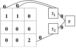
In order to obtain the MSF rooted on markers, additional vertices i.e. , are introduced. Each additional vertex is connected by the edge with a null weight to the pixels representing a marker . Furthermore, an additional root vertex is added and is connected by the null-weight edges to the vertices (see Figure 1). The minimal spanning tree of the constructed graph induces a MSF in G, where each tree is grown on a vertex . Finally, a spectral-spatial classification map is obtained by assigning the class of each marker to all the pixels grown from this marker.
0
Figure 1. An example of addition of extra vertices , and r to the image graph for the construction of an MSF rooted on
markers 1 and 2; non-marker pixels are denoted by ―0.‖
3. PROPOSED FRAMEWORK
In the proposed framework, which hereinafter is called MSF- SVM algorithm, the hyperspectral image is first classified using SVM algorithm. Then, the error rate for each class is computed as:
Er=1- PA (1)
Where and are, respectively, the error rate and the population size for class i, and N is the number of classes. In this study, class i has low accuracy if . The above valuehas been estimated by trial and error.
For this algorithm, it is in particular importance to mention that the labeling of each pixel is first decided using the algorithm. is used for classifying the image into two classes: a class with maximum value and the rest of classes. Moreover, for the condition 'if ', if the answer is negative, the pixel label can be found using the algorithm. is used to improve the class with value less than class of algorithm. This decision making process is continued using other MMSF algorithms until the answer is negative for the pixel label which is determined by SVM algorithm.
4. EXPERIMENTAL RESULTS AND DISCUSSIONS
The Berlin hyperspectral dataset was used for the experiments. Table 1 presents the main characteristics of this dataset
Dataset Berlin Sensor HyMap
Context Urban area
Spatial coverage 300×300
Spatial Resolution (m) 3.5
Number of bands 114
Number of classes 5
Table 1. The main characteristics of the Berlin dataset.
In experiments, to create a map of markers for MSF algorithm, each connected component of the SVM classification map, i.e. 8-neighborhood connectivity, is analyzed. If this region contains more than 20 pixels, 5% of its pixels with the highest estimated probability are selected as the marker for this component (Tarabalka et al., 2010). Otherwise, the region marker is formed by the pixels with estimated probability higher than a threshold . The threshold is equal to the lowest probability within the highest 2% of the probabilities for the whole image. In the next step, the image pixels are grouped into the MSF using the spectral angle dissimilarity measure, built from the selected markers (van der Meer, 2006). Moreover, in order to compare the results of the proposed MSF-SVM algorithm, we have implemented independently SVM and MMSF algorithms for image classification.
The accuracies of the classification maps are generally assessed by computing the confusion matrix using the reference data. Based on this matrix, several criteria have been used to evaluate the efficiency of algorithms (Congalton, 1991; Story and Congalton, 1986). These measures are a) the overall accuracy (OA), which is the percentage of correctly classified pixels, b) the Kappa coefficient of agreement (κ), which is the percentage of agreement corrected by the amount of agreement that could be expected due to chance alone, and c) the class-specific
1 1 0
0 0 0
0 0 2
The International Archives of the Photogrammetry, Remote Sensing and Spatial Information Sciences, Volume XLII-4/W5, 2017 GGT 2017, 4 October 2017, Kuala Lumpur, Malaysia
This contribution has been peer-reviewed.
100 95 90 85 80 75
88.3
SVM MMSF MSF-SVM
Overall Accuracy Kappa coefficient producer's accuracy, which is the percentage of correctly
classified samples for a given class.
It should be noted that, the training samples for MSF-SVM are divided in two subsets: a subset for the training SVM and a subset for finding the classes with low accuracy. We have chosen 20% exiting training samples of each class for training the SVM and the remaining for its testing.
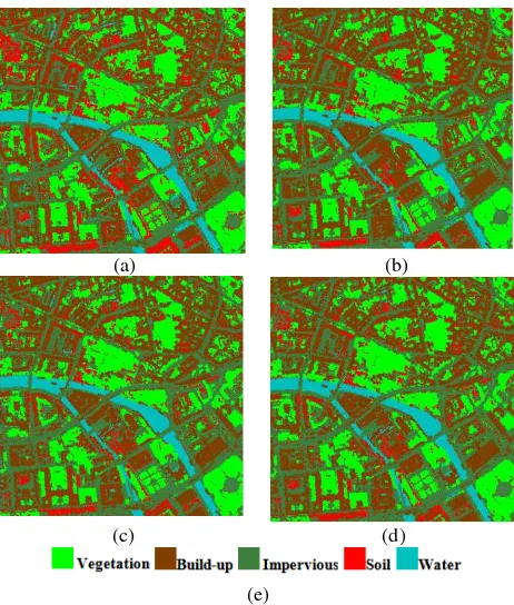
Five thematic land cover classes are identified in the Berlin dataset (see Figure 2.d): Vegetation, Build-up, Impervious, Soil and Water. For each class, we have randomly chosen 30% of the labeled samples for training and use the other 70% for testing purposes.
A pixel-based classification was performed using the multiclass SVM classifier with the Gaussian radial basis function (RBF) kernel. The penalty parameters C and (which constitute the spread of the RBF kernel) are estimated using a five-fold cross validation: C = 200 and .
Figures. 2.a, 2.b and 2.c show the classification maps of SVM, MMSF, and the proposed MSF-SVM algorithm, respectively. As can be seen, the map of the MSF-SVM algorithm contains far more homogeneous regions when compared with the maps obtained by other methods (see Figure 2.c). These results can show the importance of using spatial information throughout the classification procedure.
Figure 2. Berlin dataset: (a) SVM Classification map, (b) MMSF Classification map, (c) MSF-SVM Classification map
(d) reference map and (e) the legend.
Table 2 shows the assessment parameters of SVM classification, the overall accuracy, the kappa coefficient, and the class-specific producer's accuracy parameters. As can be seen, Build-up and Impervious classes have proposed parameter ( greater than or equal to 0.5. This increase in the parameter , as mentioned in section 3, is related to the large population and high error rate class. Also, the proposed MSF- SVM algorithm has resulted in a) up to an approximately 7%
higher rate of accuracy for the SVM, and b) up to an approximately 4% higher rate of accuracy for the MMSF in the OA (see Figure 3).
SVM MMSF MSF-SVM
OA(%) - - 85.6 88.3 92.7
(%)
- - 79.3 83.7 88.8Vegetation 2236.4 0.31 93.9 95.6 96.8
Build-up 7015.5 0.97 78.6 89.8 94.1
Impervious 7249.6 1 80.3 85.8 91.7
Soil 1055.9 0.14 85.9 89.7 86.2 Water 528.5 0.07 96.7 97.0 96.7
Table 2. The SVM assessment parameters and the classification accuracies obtained on the Berlin dataset
92.7 88.8 85.6
83.7
79.3
Figure 3. The global accuracies of different methods.
In Table 2, all the class-specific producer's accuracy rates for the proposed MSF-SVM algorithm are higher than 90%. An exception is the accuracy rates for the Soil class; these rates are slightly reduced when compared with the MMSF results. This reduce in accuracy can be due to the low number of pixels and the high dispersion of Soil class in the image. In addition, the spectral complexity of the Berlin dataset is effective in this case. Moreover, in all classes, the MMSF classification accuracy rates are much higher than those of the SVM. In Build-up and Impervious classes, (see Tab. 2), the improvements of about 16% and 11% in the producer's accuracies are obtained in compared with the SVM algorithm. This shows the importance of using spatial information in these two classes.
5.CONCLUSION
In this study, a framework for the spectral-spatial classification of hyperspectral images has proposed. In proposed framework, i.e. MSF-SVM, the hyperspectral image is first classified using SVM algorithm. Then, the MMSF spectral-spatial algorithm is used to improve the accuracy for classes with low accuracy. The experiments have been conducted using Berlin benchmark image in the hyperspectral remote sensing community acquired by HyMap in 2003. The results demonstrate that the proposed MSF-SVM algorithm generally improves the classification accuracy rates when compared to the classic SVM algorithm and the original MSF method. The kappa coefficient obtained for the MSF-SVM algorithm is approximately 5% and 9% higher than the MMSF and SVM algorithms, respectively.
ACKNOWLEDGMENTS
The authors would like to thank German Aerospace Centre (DLR) for providing the hyperspectral dataset used in this research.
A
cc
u
rac
y
(
P
er
ce
n
ta
g
e)
(a) (b)
(c) (d)
(e)
The International Archives of the Photogrammetry, Remote Sensing and Spatial Information Sciences, Volume XLII-4/W5, 2017 GGT 2017, 4 October 2017, Kuala Lumpur, Malaysia
This contribution has been peer-reviewed.
REFERENCES
Blaschke, T., Hay, G.J., Kelly, M., Lang, S., Hofmann, P., Addink, E., and Tiede, D., 2014. Geographic Object-Based Image Analysis – Towards a new paradigm. ISPRS Journal of
Photogrammetry and Remote Sensing, 87: 180–191.
Camps-Valls, G., Gomez-Chova, L., Munoz-Mari, J., Vila- Frances, J., and Calpe-Maravilla, J., 2006. Composite kernels for hyperspectral image classification. IEEE Geosci. Remote
Sensing Letter, 3, 93–97.
Carleer, A.P., and Wolff, E., 2006. Urban land cover multi-level region-based classification of VHR data by selecting relevant features. International Journal Remote Sensing, 27(6), 1035– 1051.
Congalton, R., 1991. A review of assessing the accuracy of classifications of remotely sensed data. Remote Sensing of
Environment, 37, 35–46.
Fauvel, M., Chanussot, J., and Benediktsson, J.A., 2012. A spatial–spectral kernel-based approach for the classification of remote sensing images. Pattern Recognition, 45: 381–392.
Fauvel, M., Chanussot, J., Benediktsson, J.A., and Sveinsson, J.R., 2008. Spectral and spatial classification of hyperspectral data using SVMs and morphological profiles. IEEE Translation
Geosci. Remote Sensing, 46, 3804–3814.
Gonzalez, R., and Woods, R., 2002. Digital Image Processing. 2nd ed. Englewood Cliffs, NJ: Prentice-Hall.
Huang, X., and Zhang, L., 2011. A multidirectional and multiscale morphological index for automatic building extraction from mutispectral GeoEye-1 imagery.
Photogrammetric Engineering and Remote Sensing, 77, 721-
732.
Jensen, J.R., 2004. Introductory Digital Image Processing—A Remote Sensing Perspective. 3rd ed. Upper Saddle River, NJ: Pearson Prentice-Hall.
Jimenez, L.O., Rivera-Medina, J.L., Rodriguez-Diaz, E., Arzuaga-Cruz, E., and Ramirez-Velez, M., 2005. Integration of spatial and spectral information by means of unsupervised extraction and classification for homogenous objects applied to multispectral and hyperspectral data. IEEE Translation Geosci.
Remote Sensing, 43, 844−851.
Landgrebe, D.A., 2003. Signal theory methods in multispectral remote sensing. Hoboken: John Wiley and Sons.
Negri, R.G., Dutra, L.V., and Sant’Anna, S.J.-S., 2014. An innovative support vector machine based method for contextual image classification. ISPRS Journal of Photogrammetry and
Remote Sensing, 87, 241–248.
Paneque-Gálvez, J., Mas, J.-F., Moré, G., Cristóbal, J., Orta- Martínez, M., Luz, A.C., et al., 2013. Enhanced land use/cover classification of heterogeneous tropical landscapes using support vector machines and textural homogeneity. International Journal of Applied Earth Observation and
Geoinformation, 23, 372–383.
Plaza, A., Benediktsson, J.A., Boardman, J.W., Brazile, J., Bruzzone, L., Camps-Valls, G., and Trianni, G., 2009. Recent
advances in techniques for hyperspectral image processing.
Remote Sensing of Environment, 113: S110–S122.
Rajadell, O., Garc´ıa-Sevilla, P., and Pla, F., 2009. Textural features for hyperspectral pixel classification. in IbPria09,
Lecture Notes in Computer Science 5524, 208-216.
Senthil, K.A., Keerthi, V., Manjunath, A.S., van der Werff, H.M.A., and van der Meer, F.D., 2010. Hyperspectral image classification by a variable interval spectral average and spectral curve matching combined algorithm. International Journal
Applied Earth Observation Geoinformation, 261-269.
Shackelford, A.K., and Davis, C.H., 2003. A combined fuzzy pixel-based and object-based approach for classification of high-resolution multispectral data over urban areas. IEEE
Translation Geosci. Remote Sensing, 41, 2354–2363.
Shippert, P., 2004. Why Use Hyperspectral Imagery?.
Photogrammetric Engineering and Remote Sensing, 377–380.
Shrestha, D.P., Margate, D.E., van der Meer, F.D., and Anh, H.V., 2005. Analysis and classification of hyperspectral data for mapping land degradation : an application in southern Spain.
International Journal Applied Earth Observation
Geoinformation, 85-96.
Soille, P., 2003. Morphological Image Analysis. 2nd ed. Berlin, Germany: Springer-Verlag.
Stawiaski, J., 2008. Mathematical morphology and graphs: Application to interactive medical image segmentation. Ph.D. dissertation, Paris School Mines, Paris, France.
Story, M., and Congalton, R., 1986. Accuracy assessment: A user's perspective. Photogrammetric Engineering and Remote
Sensing, 52, 397–399.
Tarabalka, Y., Chanussot, J., and Benediktsson, J.A., 2010. Segmentation and classification of hyperspectral images using minimum spanning forest grown from automatically selected markers. IEEE Translation System, Man, Cybern. B, Cybern., 40(5): 1267–1279.
Tarabalka, Y., Tilton, J.C., Benediktsson, J.A., and Chanussot, J., 2011. A Marker-Based Approach for the Automated Selection of a Single Segmentation From a Hierarchical Set of Image Segmentations. IEEE Journal of Selected Topics in
Applied Earth Observations and Remote Sensing.
Van Der Meer, F., 2006. The effectiveness of spectral similarity measures for the analysis of hyperspectral imagery.
International Journal Apply Earth Observation
Geoinformation, 8: 3–17.
The International Archives of the Photogrammetry, Remote Sensing and Spatial Information Sciences, Volume XLII-4/W5, 2017 GGT 2017, 4 October 2017, Kuala Lumpur, Malaysia
This contribution has been peer-reviewed.