Volume 25, Number 3, 2010, 325– 337
HYPOTHESIS TESTS ON HALL PERMANENT INCOME (HPI):
THE CASE OF INDONESIA
R. Maryatmo
Universitas Atma Jaya Yogyakarta (maryatmo@gmail.com)
ABSTRACT
This paper is focused on the test of Hall Permanent Hypothesis. Hall hypothesizes that economic agents have perfect information on their life time income. Since economic agents have perfect information on their life time income, they tend to hold their inter-temporal consumption to be equal. There are three ways to test the Hall hypothesis. The three ways are Dickey Fuller, Augmented Dickey Fuller, Cambell and Mankiw tests. The results are inconsistent each others. The finding tends to support that the interest rate transmission mechanism for inter-temporal consumption is not working in Indonesia. The interest rate in Indonesia tends to be higher than of the neighboring countries. The interest rate in Indonesia tends to be high because of the high inflation rate, and inefficient banking practice. It is interesting to plan further research on staggering high inflation and inefficient banking practice in Indonesia.
Keywords: Hall income permanent hypothesis, inflation, Indonesia.
INTRODUCTION
The current study aims to investigate the characteristics of random walk from the realization of consumption of Indonesians. The observation of random characteristics towards a particular phenomenon is based on Hall’s findings (1978) concerning the rela-tionship between rational expectations towards future income (rational expectation) along with the characteristics of random walk from consumption realization. Hall (1978) was first to test random walk towards a phenomenon and stated that when expectations towards future income are rational, therefore the theory of permanent income and life-cycle consump-tion indirectly endorses the characters of random walk in consumption realization.
Hall’s (1978) studies prove that consump-tive behaviors support the Permanent Income
Hypothesis (PIH). Studies from Flavin (1981), Cambell and Mankiw (1989) demonstrates that PIH is not proven or that the data does not completely support PIH. Studies in Indonesia conducted by Triandaru (2006) prove that the data do not completely support PIH. According to Triandaru, only 22% of Indonesians use information related with future income to determine the level of consumption. A study from Rao (2005) in Fiji, a developing country, also produced similar results. The conclusion is that PIH does not completely apply in the country.
Should the people be able to entirely use the most recent information for consumption decisions, therefore the present consumption level will be equivalent to the consumption level in the past added with the consumption changes that are influenced by the most recent information mentioned before. Recent infor-mation is random in nature, therefore the differences between predicting present con-sumption and concon-sumption in previous periods also become random. In general, the random walk is expressed in the following formula:
Ct+1 = Ct + t (1) Proving the characteristics of random walk for consumption decisions, apart from indicating information perfection in the economy, also indicates that people engage in reasoning when making decisions. People have considerable freedom to allocate their funds over time. Monetary policies are ineffective in influencing the economy. When information is perfect, consumers determine their long term consumption based on the permanent income during the course of their life. Should a person express optimism that he/she will gain high income in the future, this person will use future incomes for present time consumption. Conversely, when economic actors sense uncertainty of the future economy, they will tend to save for the interests of future consumption.
Income transmission towards consumption over time operates through interest rates (Mankiw, 1985). When the real interest rates are low, consumption funding becomes cheap, and people will tend to borrow more from banks for their present time consumption. Loan payments are done by using future income. Conversely with high interest rates, the opportunity cost of consumption expen-diture becomes expensive. Therefore people tend to save and use their savings for future consumption.
Not many studies of consumption over time have been conducted in Indonesia. Our
search in EBSCO electronic journal did not find a study investigating consumption over time in Indonesia. Searching in GOOGLE also did not result in research reports of consumption over time, specifically observed in Indonesia. Some regional studies can be related to consumption over time which includes Indonesian regions.
One of the studies includes the obser-vation of financial integration in Australia and Asia (Brouwer, 1996). A few countries were observed by Brouwer in addition to Australia including Hongkong, Japan, Taiwan, Thailand, Singapore, Indonesia, and Malaysia. The study concluded that financial integration had taken place in Australia and Asia. Moreover, the researcher also concluded that no clear relationships between economic openness with economic performance was established, indicated by savings and investment performance. This implies that transmission over time has not operated perfectly as well as its influence towards the performance of consumption. Kim et al (2005) studied the influence of financial integration towards the spread of consumption risks among countries in East Asia including Indonesia. The stock market and credit market played a minor role in spreading consumption risks. In line with Brouwer’s findings, Kim (2005) and Rao (2005) demonstrated that monetary transmission to the real sector did not proceed effectively.
MODEL AND APPROACH
To introduce the consumption over time model we would firstly introduce the simplest form of the model, namely the two period model. It is assumed that economic actors live in two periods, the present (t) and the future (t+1). Economic actors acquire adequate information to decide on their present consumption (Ct) or future consumption (Ct+1). Economic actors hold the utility functions over time as presented below (Waldman, 2003, pp 106-118)
U = f (Ct, Ct+1) (2)
Maximum consumer satisfaction is achieved when the consumers are able to effectively decide the allocation of their consumption. The substitution between consumption levels over time is referred to as Marginal Rate of Time Preference (MRTP) and can be formulated as the following.
MRTP =
1 t
t
1 t
t
C U C
U
dC dC
(3)
In order to elevate levels of satisfaction, consumers encounter a budget constraint over time. Consumers obtain income for each period. Income Mt for period one, and income Mt+1 for period two. It is assumed that income in period two, referring to the period resembling the future, is certain. Consumers are entitled to make higher levels of consumption by borrowing money. The interest rates charged is (Rt). Consumers could save with the equivalent amount of interest (Rt) for future consumption. If consumers borrow money for present consumption, the consumer must return the principal in addition to the interests costs in the future. If consumers save in the present, they have higher purchasing power in the future. His savings and interests will be added as income in the next period. Savings can be defined as
the remaining income from present consumption.
St = Mt– pt Ct (4)
The notation pt serves as the consumption price index. Equation (4) can also imply that savings (St) indicates a negative value, should the consumer borrow for present consumption.
The total amount of money used for future consumption refers to future income (Mt+2) added with savings (St) added with saving interests (RtSt). In the case of negative savings, it implies that the consumer borrows, and he is required to return the loan together with its interest in the future. The payment of loans and loan interests reduce his future consumption rates. Future consumption is expressed in the following equation:
pt+1 Ct+1 = Mt+1 + St + RtSt = Mt+1 +
(1 + Rt) St (5)
Noting that Rt refers to interests, when equation (4) is substituted with equation (5), therefore the new formula below is produced.
pt+1 Ct+1 = Mt+1 + (1+ Rt) (Mt– pt Ct)
= Mt+1 + (1+ Rt) Mt - pt (1+ Rt) Ct
The equation above can also be formulated differently as displayed below.
pt+1 Ct+1 + pt (1+ Rt) Ct = Mt+1 +
(1+ Rt) Mt (6)
Optimization of constrained utility function can be achieved with the Lagrange Multiplier method. The Lagrange equation is expressed as follows:
Max LU(C1,C2)(Mt1(1Rt)Mt
0
The aforementioned balance requirement stated that currently, the amount of money used for present consumption produces the same satisfaction with the amount of money used for future consumption. Equation (10) and (11) results in present consumption demands (Ct), and future consumption demands, with each serving as a function from present income (Mt), future income (Mt+1), interest (Rt), and price (pt).
ECONOMETRIC AND STATISTICAL TESTS
The following sub-chapter will discuss the required econometric and statistical tests. The econometric tests used in the study consist of those performed by Hall and applied by Rao (2005), as well as additional tests which are the Dickey Fuller tests and Augmented Dickey Fuller tests as well as Co integration tests (Gujarati, 2003). The statistical tests will include t-tests and F-test. These tests are to be explained in the following sections respectively.
1. Dickey Fuller Test
The Hall random walk tests basically observe the relationship between marginal consumer satisfactions over time. To perform
the Hall test approach, a number of testing alternatives are considered for example Dickey Fuller test and Augmented Dickey Fuller test, in addition to the Hall test itself. Numerous complementary tests and Hall tests are consecutively elaborated. Because Hall (1978) assumed that information is perfect, and that consumers acquire the ability to predict their future income levels, consumption levels are likely to remain constant. Hall simplified equation (11) to become equation (1). Equation (1) can be expressed in a much simpler form by adding a coefficient and delaying the time one period backward as displayed below.
Ct = β Ct-1 + t (12) Equation (12) will be equivalent to equation (1) when β = 1. Equation (12) or (1) will indi-cate random walk when β=1 is proven. The requirement of β=1 states that past consump-tion is equivalent to present consumpconsump-tion, except in cases of random shock as large as t. Equation (13) is basically identical to equation (12) if =(β–1). Should equation (12) require the condition of β=1, this implies that equation (14) needs to be proven with =0. To prove equation (13) the following hypothesis is required.
H0 : = 0 HA : ≠ 0
Such tests basically resemble the application of the Dickey Fuller test (Gujarati, 2003).
2. Augmented Dickey Fuller Test
has the tendency to produce residuals (t) that are auto-correlative. To eliminate or reduce the tendency for autocorrelation, Dickey Fuller introduced the autoregressive variable in equation (13). It is also likely that autocorre-lation is caused by trends in the consumption variable. To eliminate the element of trend, it is possible to add the variable trend to equation (13). The Augmented Dickey Fuller equation is formulated as below.
Ct = 0 + 1 t + 2 Ct-1 +iCt-i + t (14) The proposed hypothesis is identical with the hypothesis that performs tests for equation (13).
3. Hall Tests
Cambell and Mankiw (1989) performed the Hall hypothesis test and made a solution for equation (10) and (11) to obtain a consumption equation as a function of present and future income, interest, and price. Cambell and Mankiw subsequently assumed that a number of consumers (1–) are forward looking and make consumption decisions based on the permanent income they possess, while the remaining () make consumption decisions based on the consideration of the level of present income possessed. Should intertemporal processes occur, therefore the random walk hypothesis tests can be per-formed through the following specified model.
Ct = µ + Mt + (1–) Rt + t (15) The notation indicates the substitution elasticity parameter and Rt represents real interest rate. When the actual interest becomes a transmission of income over time, the coefficient parameter (1–) should be signi-ficant and in equivalent to zero. Considering that determining the credit of developing countries is not determined by interest (Rt) but by other variables for example the debtor’s status, and because the bank’s interest is usually controlled by the monetary powers, the variable of interest (Rt) in Cambell and
Mankiw’s paper approach uses an instru-mental variable (IV). The approach utilizing the instrumental variable becomes an alternative towards the interest variable that becomes a transmission of people purchase power over time. Rao (2005) applied this model for the Fiji case. Considering that the study period in Fiji involved the period where goods and services tax had been introduced, therefore the model included dummy variables within the model that indicates differences of observation prior to and following the implementation of tax. The econometric model is presented as follows.
lnCt = µ + lnMt + (1–) Rt + β T DUMt + t (16) The model is specified as a non-linear model to enable estimations using the Ordinary Least Squares model by creating linearity and using its log values. The focus of the study remains to test transmission of interest in the Fiji economy, using the t-test towards the significance coefficient (1–) .
4. Normality Tests
Numerous statistical tests assume that the basic distribution probability resembles a normal distribution. Statistical parameters that are to be tested are assumed to have a normal distribution. Statistical parameters are assumed to have a normal distribution because the statistical parameters are a function of the residuals that are assumed to have a normal distribution. Therefore, numerous new statis-tical tests can be performed when the assumption of normality for the residuals are proven. Normality tests testing the residuals of an equation with a normal distribution are very important in the process of statistical tests.
2003, pp 148-9). Among the characteristics of a normal distribution are a Skewness (S) of zero (0), and a Kurtosis (K) of three (3). The JB formula test is expressed as follows.
The degree of freedom from the JB statistic is as large as two. If the probability value of the JB statistic is low, this means that the JB value is statistically considered equal to zero, the researcher can reject the hypothesis that the residuals have a normal distribution. If the probability value is high, it is happen when the JB statistic is high, the researcher cannot reject the assumption that residuals have a normal distribution.5. Co-integration Tests
A new regression estimation outcome can be understood as the estimation outcome when the regression outcome is not spurious (Thomas, 1997 pp 426). In order to ensure that the regression is not spurious, numerous methods can be applied for example 1) the variables that are estimated are stationery variables; 2) in cases where the regressed variable is non stationery, however the variable indicates the same level of integration namely 1 degree, therefore the estimation can be made through a co integration approach. The equation can be co integrated when the residuals from the equation is stationery.
Co integration tests can be performed using the unit square tests as follows (Gujarati, 2003, pp 823).
t = t-1 + µt (18) The above residual is assumed to be stationery when the autocorrelation equation (18) pro-duces an autocorrelation coefficient in equivalent to one (≠ 1), or in other words if ≠ 0. Co integration tests can be performed with the following hypothesis tests.
H0 : = 0 HA : ≠ 0
Should it be statistically proven that theta () is in equivalent to zero, implying that the rho autocorrelation coefficient () is in equivalent to one, therefore it can be concluded that the residuals tend to be convergent and stationery, and therefore it can be indirectly concluded that the long term equation is co integrated (Engle, and Granger, 1991, pp. 8-15)
6. t Tests
T tests are performed in order to prove that each independent variable statistically indicates a significant influence towards the dependant variable. T Tests are performed with statistical tests with the null hypothesis as a parameter equivalent to zero. The alternative hypothesis is that the parameter coefficient is equal to zero. The hypothesis is formally expressed as follows.
H0 : 1 = 0 HA : 1 ≠ 0
The value of the t statistic can be calculated by using the following formula (Wallpole, 1993)
If the calculated t from formula (20) is higher than that of the t table, for a particular confidence level and for a certain degree of freedom, it is proven that the coefficient parameters of the estimation is not statistically equal to zero. It implies that the independent variable statistically influences the dependent variable. If the t calculated from formula (20) is smaller than that of the table t, with a particular confidence level and the degree of freedom, it is proven that the estimated parameter coefficient is equal to zero. Because the estimated regression parameter is equal to zero, the effect of the independent variable towards the dependent variable is statistically insignificant.
7. F test
F Tests are used to prove that the effect of the independent variable towards the dependent variable is statistically significant. F tests are based on the F distribution referred to as Explained Sum Squares (ESS) towards the Residual Sum Squares (RSS), and each com-ponent divided with the degree of freedom. The F statistic formula can be expressed in the following formula (Wallpole, 1993) calculate the related component values. F tests can be performed by proposing the following hypothesis.
H0 : 0 = 1 = 2 = ... n = 0 HA : 0≠ 1 ≠ 2≠... n ≠ 0
Should the calculated F be larger than the F in the table, with the degree of freedom, and a particular confidence level, therefore it can be concluded to reject the assumption that the regression parameter coefficient equals to zero, and accept that statistically all regression parameter coefficients do not equal to zero. The rejection of the null hypothesis implies that statistically, the variance of the independent variable is simultaneously able to explain the variance in the dependent variable. Conversely should the F be smaller than the F in the table, with the confidence level, and degree of freedom, therefore the hypothesis that states that the regression parameter coefficient equals to zero cannot be rejected. Because statistically all regression parameter coefficients equal to zero, therefore the effect of the independent variable is insignificant towards the dependent variable.
DATA AND CONSUMER ABILITY TO USE INFORMATION AND INTEREST TRANSMISSION
The data used in the study comprise of quarterly data from the first quarterly year 1983 until two quarterly years of 2008 downloaded from the Bank Indonesia website (http://www.bi.go.id/). The data downloaded from the BI website used in this research consist of the data variable consumption, income, interest, and inflation.
The variable interest is approached using the real interest which refers to the difference between nominal interests with the inflation rate. The data on nominal interest used is the three month interest deposit. The three month deposit interest is used as an approach towards nominal interest because the three month deposit is one of the bank products that is largely requested by depositors and is relati-vely sensitive towards interest change, meanwhile inflation rates are reduced from the Consumer Price Index variable. The last variable is time, which is approached using physical time. The first quarterly of 1983 is represented by one, and the second quarterly of 1983 is represented by two and etc.
According to Hall (1978) consumers are able to make estimations of their future income. Consumption expenditures over time tend to be constant. Consumers use their inco-me over tiinco-me for an equal level of con-sumption over time. The level of concon-sumption tends not to change over time. Present consumption expenditures are likely to be equal with past time consumption added with the change of consumption caused by the change of information obtained when making a consumer decision. The statement above can be mathematically represented by equation (1).
In an econometric sense, equation (1) also states that auto correlative consumption over time is very high. Present consumption is highly influenced by past time consumption. Hall (1978) stated that the level of past time consumption is equivalent to the level of present consumption, therefore it can be said that the level of auto correlative consumption equals to one. Empirically, the data from Indonesia from the first quarterly 1983 to the second quarterly 2008 demonstrates a strong relationship between consumptions over those periods. Because the data is presented through quartiles, therefore the correlation of consumption over time is made in two versions. The first version is the version for
relationship of consumption between quartiles, while the second version is the relationship of consumption between years. The correlation of consumption is displayed in Table 1 and Graphic 1 as follows.
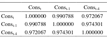
Table 1. Correlation of Consumption Over
Time
Const Const-1 Const-4 Const 1.000000 0.990788 0.972067 Const-1 0.990788 1.000000 0.974301 Const-4 0.972067 0.974301 1.000000
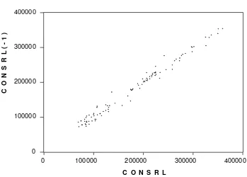
Observing the figure and table above, the relationship between consumption over time is clearly established, therefore it could be said that present consumption is equivalent to past consumption. In terms of the correlation values, the relationship is very strong. The value for correlation is 0.99 and 0.97, which are consecutively presented for the relationship of present consumption with consumption in the last quarterly (t-1), and past year consumption (t-4). The figure also demonstrates the relationship between present consumption and consumption in past quartiles which is also very strong and forms a 45 degree diagonal. From the correlation values it is clear (although its values not large), that time brings upon change. The correlation for consumption between quartiles is stronger compared to consumption between years. However the figure and the values may be deceiving in some sense. Processes of formal verification are largely required. The approach of Dickey Fuller demonstrates that does not equal to zero, as displayed in the following estimation outcomes.
D(CONSRL) = 0.01461663763*CONSRL(-1) (2.669283)*
R squared = 0.001764 Adjusted R-Squared = 0.001764
0 100000 200000 300000 400000
0 100000 200000 300000 400000
C O N S R L
C
O
N
S
R
L
(
-1
)
. .
Figure 1. Correlation of Consumption Over Time
The values in the brackets represent the values of the calculated t. The asterisk above the brackets represents the calculated t of 2.66 which is larger than the t in the table on the risk level of 5 percent. If the calculated t is larger than the table t this implies that theta () is in equivalent to zero. Past time consumption is in equivalent to present time consumption, and the Hall hypothesis is not proven. Interest transmission for consumption over time did not occur. The DF tests indicate a weakness. The DW indeed indicates a value of 1.8, which implies that no first order autocorrelation is present, however the LM autocorrelation tests indicate that the autocorrelation for orders larger than one, is present in the estimation outcome for the residuals, therefore indicating a bias estimation outcome (Gudjarati, 2003, pp 452). The DF Model presents its own fundamental weaknesses, because the potential of autocorrelation within itself. In addition to the normality tests with the Jarque Berra (JB) statistical values of 14.85 and p as large as
0.0005, it fails to prove the basic assumption that the residuals are normally distributed, therefore making the results of other statistical tests dubious to account for.
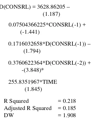
Although the results of the statistical tests are unreliable, however it remains plausible to understand that present real consumption is not equal to past time consumption. In reality the consumption level continues to increase in line with the increase of production and income. It becomes necessary to further test the statistical significance of these increases. To take account of the lack of validity of the Hall statistical tests using the DF test approach, the Augmented Dickey Fuller (ADF) approach is introduced. The ADF tests include the lag dependent variable in order to reduce or eliminate autocorrelation between residuals.
D(CONSRL) = 3628.86205 – (1.187)
0.07504366225*CONSRL(-1) + (-1.441)
0.1716032658*D(CONSRL(-1)) – (1.794)
0.3760622364*D(CONSRL(-2)) + -(3.848)*
255.8351967*TIME (1.845)
R Squared = 0.218 Adjusted R Squared = 0.185
DW = 1.908
The JB statistic demonstrates a relatively low value of 3.06, with a p of 0.19 indicating that the residuals are normally distributed as assumed by the Ordinary Least Squares approach. Furthermore statistical tests that are based upon the normality assumptions can be performed. The theta coefficient () is as large as (-0.0750), with the calculated t (-1.441). The calculated t will be equivalent to the table t with a risk level of 15.27%. If the maximum risk level was established at 5%, the calculated t would be larger compared to the t in the table. Theta is not significantly different with zero, therefore the autocorrelation coefficient equals to one. This implies that the present consumption level is not significantly different with zero, therefore the autocorrelation coefficient equals to one. This implies that the present consumption level with the past quarterly consumption level added with unexpected values (residual) occurred at the moment the consumption decision was made. Although the consumption value from time to time experiences an increase, however the increases for each quarterly are statistically insignificant.
The third Hall test approach is used in the Cambell-Mankiw model (1989). The initial estimation outcome was free from heteros-cedasticity although it experienced
autocorre-lation. When overcoming the issue of autocorrelation with the weighted approach towards its autocorrelation, or took into account the variable of time trends, the first degree autocorrelation tended to disappear. Although cured from the ills of autocorrelation however the remaining results were marked with non-normal residuals. Further obser-vations demonstrate that the non-normal residuals are primarily caused by the crisis period in 1997 and 1998 where consumption tends to sharply increase from average. This tendency can be understood, because when dealing with a crisis and uncertainty, consumers tend to buy up goods before prices increase. Expectation towards the crisis increases the consumption to reach levels above average. Non normality is also supported by the presence of extreme data in March. Each march the consumption levels significantly reduces below the average. Such declines are possibly attributed to seasonal fluctuations. Seasonal weightings on March are too large. The cured estimation outcome from first degree autocorrelation is as follows.
LOG(CONSRL)-RHO*LOG(CONSRL(-1)) =
1.1286887 + 0.6852833511*(LOG(YRL) – (2.227)* (5.517)*
RHO*LOG(YRL(-1))) – 0.00257127838* (-1.416)
((RN-RHO*RN(-1))-(INF-RHO*INF(-1))) +
0.002101146332*TIME (3.437)*
R2 = 0.880 R2 Adj = 0.876 DW = 1.946
5 percent. The result of the first study is interesting to discuss as the coefficient for present consumption is 0.685. This implies that 69 percent of Indonesians behave in line with Keynes’s theory. As much as 69 percent of Indonesians perform consumption patterns based on present consumption. While 31 per-cent of the remaining behave intertemporally. They perform their consumption patterns by considering future income. The results of the study are closely related with the findings of Triandaru (2006) that demonstrates that 68 of Indonesians display consumption behaviours in accordance with Keynes theory. The remaining 32 percent of Indonesians display consumption patterns in accordance with the Permanent Income Hypothesis theory. Triandaru conducted a study with annual data from the period 1980-2004. The findings are identical with the findings of the value of marginal rate of consumption (mpc) of Indo-nesia with Keynes’s approach that demons-trates the mpc value as large as 70 percent (Maryatmo, 2004). A study from Rao (2005) concerning proportion of the people who make consumption decisions based on present income information is as large as 61 to 71 percent. This implies that most of the Fiji people act in accord with the predictions of Keynes. While the remaining (between 29-39 percent) decide their level of consumption based on income information over time.
The estimation outcome for the interest’s parameter and the elasticity substitution indi-cates that it is in line with expectation theory. If interest rates increase, present consumption rates will decline. The increase of interest rates implies an increase in consumption costs. If the cost of consumption increases, the rate of consumption will decline. However, the magnitude of the estimation of the interest coefficient parameter and elasticity substitutions is statistically insignificant. This implies that interest transmission for purchase power over time does occur. Stimulus of interest is inadequate to trigger change in
consumption. Obstacles related with credit, causes the interest to be useless in influencing consumption.
Obstacles related with credit can be observed from the perspective of supply or demand. Obstacles from the supply may occur because Indonesian banks are inefficient in executing their roles as intermediary financial institutions. The interest that is offered by the banks is relatively high compared to the credit interest rates in neighboring countries. The high interest rates in banks are generally caused by the high inflation in Indonesia, and the use of interest as the basis of bank income (Goeltom, 2007, pp 280).
Elasticity of substitutions is statistically insignificant. The low elasticity of substitutions implies the very low intertem-poral transmission. Interest coefficient esti-mation outcomes and elasticity of substitutions is as large as 0.00257. If the estimation results of lambda, that represents the proportion of people making consumption decisions using considerations of present time, is as large as 0.685, the value of elasticity of substitutions is as large as minus 0.00817. The increase of present consumption as large as one percent would be substituted with the reduction of future consumption with a very small percentage as large as 0.00817. Consumption transmission over time does not occur, because of credit obstacles and interest transmission. The absence of income transmission over time also indicates that the information is not perfect, therefore consumers are not able to appropriately predict their future income.
CONCLUSIONS
based on information of their current income. Interest transmission is also inadequate in supporting the transmission of people purchase power over time. The high interest rates cause the opportunity cost of con-sumption to be expensive. The high interest rates are triggered by the high inflation in Indonesia, and also because of the inefficiency of banks in Indonesia.
Several approaches for proving Hall hypothesis which predicts that people use information to determine their level of con-sumption over time resulted inconsistent conclusion. The inconsistent results are primarily caused by the different assumptions that base those numerous approaches. The more realistic conclusion is that Hall hypothesis simply does not apply in Indonesia. Constraints on interest transmission are one of the causal factors for not allowing intertemporal consumption transmission to take place. Credit constraints which dampened the transmission on intertemporal consumption is an interesting agenda for further research. It would be an interesting topic of future research is about high inflation in Indonesia that eventually stimulates high nominal interest rates.
REFERENCES
Brouwer, G., 1996. “Consumption and liqui-dity constraints in Australia and East Asia: Does financial integration matter?” Research Discussion Paper, Reserve Bank of Australia.
Cambell, J., Y., and Mankiw, N., G., 1989.
“Consumption income and interest rates: Reinterpreting the time series evidence”, Working Paper No. 2924, National Bureau of Economic Research, Cam-bridge, MA.
Engle, R., F., and C., W., J. Granger. 1991. Long-Run Economic Relationships, Reading in Cointegration, Oxford University Press, New York,
Flavin, M. A., 1981. “The adjustment of consumption to changing expectation about future income”, Journal of Political Economi, 89, 974-1009.
Goeltom, Miranda, S., 2007. Essays in Macroeconomic Policy: The Indonesian Experience”, Gramedia, Jakarta.
Gujarati, Domodar, N., 2003. Basic Econo-metrics, International Edition, 4th ed., McGraw-Hill, Singapura.
Hall, R.E., 1978. “Stocastic implications of the life cycle-permanent income hypothesis: Theory and evidence”, Journal of Political Economy, 86: 971-87.
Kim, Soyoung, Sunghyun, H., Kim, and Yunjong Wang. 2005. “Financial inte-gration and consumption risk sharing in
East Asia”, Research Discussion Paper, Research Institute for SUPEX Mana-gement: Republic of Korea.
Mankiw, Gregory, N., 1985. “Consumer durables and the real interest rate”, The Review of Economics and Statistics, Vol LXVII (3).
Maryatmo, R., 2004. “Dampak moneter kebi-jakan defisit anggaran pemerintah dan peranan asa nalar dalam simulasi model makro-ekonomi Indonesia (1983:1– 2002:4) [“The impacts of fiscal deficit policies and the role of rational expectation on simulation of Indonesian macroeconomic model (1983:1-2002:4)]”. Buletin Ekonomi Moneter dan Perbankan, September.
Rao, Bhaskara, B., 2005. “Testing Hall’s permanent income hypothesis for a developing country: the case of Fiji”, Applied Economics Letters, 12: 245-248 Serven, Louis, 1999. “Terms-of-trade shocks
and optimal investment: Another look at the Laursen-Metzler effect “, World Bank Policy Research Working Paper, No 1424, World Bank.
Econo-mics, Manchester Metropolitan Univer-sity, Addison Wesley Longman, 1st ed. Triandaru, S., 2006. Penerapan Fungsi
Kon-sumsi Tradisional dan Life Cycle-Perma-nent Income Hypothesis pada Konsumsi Indonesia Tahun 1980-2004 [Application of Traditional and Life Cycle Permanent Income Hypothesis Consumption Function on Indonesian Cases in 1980-2004
Periods] Penelitian tidak dipublikasikan, didanai oleh Fakultas Ekonomi Univer-sitas Atma Yogjakarta.
Waldman, Don, E., 2003. Microeconomics, International Edition, Pearson, Boston. Walpole, Ronald W., and Raymond H. Myers,