For your convenience Apress has placed some of the front
matter material after the index. Please use the Bookmarks
Contents at a Glance
About the Authors ...
xiii
About the Technical Reviewer ...
xv
Acknowledgments ...
xvii
Introduction ...
xix
Chapter 1: Business Intelligence Basics
■
...
1
Chapter 2: Visio Services
■
...
59
Chapter 3: Reporting Services
■
...
143
Chapter 4: Business Connectivity Services
■
...
187
Chapter 5: Excel Services
■
...
247
Chapter 6: PerformancePoint Services
■
...
305
xix
Introduction
In working with SharePoint and with BI, we frequently found that there was no single source of information that could address the needs of both database administrators (DBAs) and SharePoint administrators and developers. With that in mind, we decided to write one.
In fairness, given the pace of the technology we deal with, it’s very difficult to find one source for it all. But, in order to deliver solutions with these modern platforms, one needs to know core business intelligence (BI) concepts as well as core SharePoint BI concepts.
SharePoint is becoming the de facto choice for delivery of BI products for Microsoft. This has been happening ever since the introduction of Visio Services, Business Connectivity Services, Reporting Services, Excel Services, PerformancePoint Services and, as icing on the cake, Power View for interactive analytics.
Even if you are an experienced .NET developer, you’ll find it difficult to find a single book that teaches enough of all these technologies and BI concepts. That’s why we put this book together—to address that unique and fascinating area that is the intersection of BI and SharePoint 2013. The first chapter gets you familiar with enough BI concepts to get you going, even if you have no background in BI. Expert DBAs can skip this chapter. The subsequent chapters focus on each of the core SharePoint BI concepts one by one, and they give you enough examples to explore each of these topics in detail. Moreover, we made it a point not to ignore the administrative side of things. In each chapter, we introduce you to the various facilities in central administration, and we also look at the PowerShell commands relevant to these features.
Business Intelligence Basics
This chapter presents the basics of business intelligence (BI). If you’re an experienced data-warehouse expert, you might want to skip this chapter, except for the section at the end that introduces Microsoft SharePoint 2013 BI concepts. But, because most readers will be SharePoint experts, not data-warehouse experts, we feel it necessary to include the fundamentals of data warehousing in this book. Although we can‘t cover every detail, we’ll tell you everything you need to get full value from the book, and we’ll refer you to other resources for more advanced topics.
What Will You Learn?
By the end of this chapter, you’ll learn about the following:
The essentials of BI •
The OLAP system and its components •
Microsoft SQL Server 2012 BI tools •
SharePoint 2013 BI components •
Software Prerequisites
You’ll need a basic understanding of databases and the relevant tools to get the most out of the topics in this book. You’ll also need the software listed here:
SharePoint Server 2013 Enterprise Edition •
SQL Server 2012 Developer Edition and its BI tools, SSDT (SQL Server Development Tools, •
formerly known as BIDS, or Business Intelligence Development Studio) for Microsoft Visual Studio 2010
SQL Server 2012 Developer Training Kit, available for download at •
http://www.microsoft.com/en-us/download/details.aspx?id=27721
AdventureWorks DB for SQL Server 2012, available for download at •
http://msftdbprodsamples.codeplex.com/releases/view/55330
Visual Studio 2012 Professional Edition, trial version available for download at •
2
Microsoft SharePoint Designer 2013, available for download at •
http://www.microsoft.com/en-us/download/details.aspx?id=35491
If you prefer to use Express editions of Visual Studio and SQL Server instead of the full •
versions, you can download them from http://www.microsoft.com/express/.
Note
■
At the time of writing, Microsoft had not released SQL Server 2012 Business Intelligence project templates for
Visual Studio 2012. Hence, we use Visual Studio 2010 throughout this book to develop BI projects, and Visual Studio 2012
to develop solutions specific to SharePoint 2013.
Introduction to Business Intelligence
Effective decision-making is the key to success, and you can’t make effective decisions without appropriate and accurate information. Data won’t do you much good if you can’t get any intelligent information from it, and to do that, you need to be able to analyze the data properly. There’s a lot of information embedded in the data in various forms and views that can help organizations and individuals create better plans for the future. We’ll start here with the fundamentals of drilling down into data—how to do it and how you can take advantage of it.
I couldn’t resist including a picture here that highlights the benefits of BI. (See Figure 1-1.) This drawing was presented by Hasso Plattner of the Hasso Plattner Institute for IT Systems at the SIGMOD Keynote Talk. (SIGMOD is the Special Interest Group on Management of Data of the Association for Computing Machinery.)
Why Intelligence?
Chances are you’ve seen the recommendations pages on sites such as Netflix, Wal-Mart, and Amazon. On Netflix, for example, you can choose your favorite genre, and then select movies to order or watch online. Next time you log in, you’ll see a “Movies you’ll love” section with several suggestions based on your previous choices. Clearly, there’s some kind of intelligence-based system running behind these recommendations.
Now, don’t worry about what technologies the Netflix web application is built on. Let’s just try to analyze what’s going on behind the scenes. First, because there are recommendations, there must be some kind of tracking mechanism for your likes and dislikes based on your choices or the ratings you provide. Second, recommendations might be based on other users’ average ratings minus yours for a given genre. Each user provides enough information to let Netflix drill down, aggregate, and otherwise analyze different scenarios. This analysis can be simple or complex, depending on many other factors, including total number of users, movies watched, genre, ratings, and so on—with endless possibilities.
Now consider a related but different example—your own online banking information. The account information in your profile is presented in various charts on various timelines, and so forth, and you can use tools to add or alter information to see how your portfolio might look in the future.
So think along the same lines, but this time about a big organization with millions of records that can be
explored to give CIOs or CFOs a picture of their company’s assets, revenues, sales, and so forth. It doesn’t matter if the organization is financial, medical, technical, or whatever, or what the details of the information are. There’s no limit to how data can be drilled down into and understood. In the end, it boils down to one thing—using business intelligence to enable effective decision making.
Let’s get started on our explorations of the basics and building blocks of business intelligence.
Understanding BI
Just about any kind of business will benefit from having appropriate, accurate, and up-to-date information to make key decisions. The question is, how do you get this information when the data is tightly coupled with business—and is continually in use? In general, you need to think about questions such as the following:
How can you drill down into tons of information, aggregate that information, and perform •
mathematical calculations to analyze it?
How can you use such information to understand what’s happened in the past as well as •
what’s happening now, and thereby build better solutions for the future?
Here are some typical and more specific business-related questions you might have to answer:
What are the newly created accounts this month? •
Which new users joined this quarter? •
Which accounts have been removed this year? •
How many vehicles have we sold this year, and what’s the new inventory? •
How many issues have been addressed this week in the command center? •
What is the failure rate of products in this unit? •
What are the all-time top 10 stocks? •
Can you rank these employees in terms of monthly sales? •
4
What kind of system could provide the means to answer these questions? A comprehensive business intelligence system is a powerful mechanism for digging into, analyzing, and reporting on your data.
Note
■
Business intelligence is all about decisions made effectively with accurate information in a timely manner.
Data mostly has a trend or a paradigm. When you’re looking at the data, you might begin to wonder, “What if....” To answer this question, you need the business intelligence mechanism. Understanding the basics of BI or data-warehouse modeling helps you achieve accurate results.
Every industry, organization, enterprise, firm, or even individual has information stored in some format in databases or files somewhere. Sometimes this data will just be read, and sometimes it needs to be modified and provide instant results. In such cases, one significant factor is the size of the data. Databases that yield instant results by adding, editing, or deleting information deal with transactional1 data. Such information needs a quick turnaround from the applications. In such cases, users seek or provide information via the UI or another source, and the result of any subsequent read, publish, edit, or even delete must happen instantly. Transaction results must also be delivered instantly, with low latency. A system that can deliver such instant results usually is based on the model called Online Transaction Processing, or just OLTP.
OLTP vs. OLAP
Online Transaction Processing (OLTP) systems are more suitable for handling transactional data and optimized for performance during Read/Write operations specifically for a faster response. On the other hand, Online Analytical Processing (OLAP) systems are read-only (though there can be exceptions) and are specifically meant for analytical purposes. This section explores these two systems in more detail.
Online Transaction Processing System
Data in the OLTP model is relational, and it is normalized according to database standards—such as the third or fourth normal form. Normalization involves splitting large tables into smaller tables to minimize redundancy and dependency in data. For example, instead of storing an employee’s department details in the employee table itself, it would be better to store the same information in a department table and link it to the employee table.
An important factor in the OLTP model is that data doesn’t repeat in any fashion; hence, it is arranged into more than one table. In this way, transactions involve fewer tables and columns, thus increasing performance. There are fewer indexes and more joins in this model, and the tables will hold the key information.
Figure 1-2 shows a basic OLTP system.
Note
■
We strongly recommend you download and install the AdventureWorks sample database from
msftdbprodsamples.codeplex.com/downloads/get/417885
. You’ll get the most out of this chapter and the others if
you can follow along.
OLTP is not meant for slicing and dicing the data, and it’s definitely not meant to be used to make key decisions based on the data. OLTP is real-time, and it’s optimized for performance during Read/Write operations specifically for a faster response. For example, an OLTP system is meant to support an airline reservation system that needs to publish airline schedules, tariffs, and availability and at the same support transactions related to ticket reservations and cancellations. The system cannot be used for analysis because that would degrade the performance of routine transactions. Moreover, a normalized structure is not suitable for analysis (for example, revenue analysis for an airline) because this involves joins between various tables to pull relevant information, leading to increased query complexity.
Take a look at Figure 1-3. Notice how information is limited or incomplete. You cannot tell what the numbers or codes are for various columns. To get more information on these values, you need to run a query that joins this table with others, and the query would become bigger and bigger as the number of relational tables increases.
Figure 1-2. HR Relational Tables from the AdventureWorks database
6
On the other hand, it would be very easy to query the table if it were a little bit denormalized and had some data pre-populated, as shown in Figure 1-4. In this case, the number of joins is reduced, thereby shortening the T-SQL query. This simplifies the query and improves the performance. However, the performance depends on the efficiency of indexing. Further, denormalizing the tables causes excessive I/O.
Caution
■
As you can see in Figure
1-4
, the T-SQL query would be simplified, but denormalized tables can cause
excessive I/O because they contain fewer records on a page. It depends on the efficiency of the indexing. The data and
indexes also consume more disk space than normalized data.
You might wonder why you can’t simply run these queries on your OLTP database without worries about performance. Or create views. Simply put, OLTP databases are meant for regular transactions that happen every day in your organization. These are real-time and current at any point of time, which makes OLTP a desirable model. However, this model is not designed to run powerful analyses on these databases. It’s not that you can’t run formulas or aggregates, it’s that the database might have been built to support most of the applications running in your
organization and when you try to do the analysis, these applications take longer to run. You don’t want your queries to interfere with or block the daily operations of your system.
Note
■
To scale operations, some organizations split an OLTP database into two separate databases (that is, they
replicate the database). One database handles only write operations, while the other is used for read operations on the
tables (after the transactions take place). Through code, applications manage the data so that it is written to one database
and read for presentation from another. This way, transactions take place on one database and analysis can happen on
the second. This might not be suitable for every organization.
So what can you do? Archive the database! One way that many organizations are able to run their analyses on OLTP databases is to simply perform periodic backups or archive the real-time database, and then run their queries on the disconnected-mode (non-real-time) data.
Note
■
A database that has been backed up and repurposed (copied) for running analyses might require a refresh
because the original source database might have had data updated or values changed.
Good enough? Still, these OLTP databases are not meant for running analyses. Suppose you have a primary table consisting of information for one row in four different normalized tables, each having eight rows of information—the complexity is 1x4x8x8. But what if you’re talking about a million rows? Imagine what might happen to the
performance of this query!
Note
■
The data source for your analysis need not be OLTP. It can be an Excel file, a text file, a web service, or
information stored in some other format.
We must emphasize that we are not saying that OLTP doesn’t support analysis. All we are saying is that OLTP databases are not designed for complex analysis. What you need for that is a nonrelational and nonlive database where such analysis can be freely run on data to support business intelligence.
To tune your database to the way you need to run analyses on it, you need to do some kind of cleaning and rearranging of data, which can be done via a process known as Extract, Transform, and Load (ETL). That simply means data is extracted from the OLTP databases (or any other data sources), transformed or cleaned, and loaded into a new structure. Then what? What comes next?
The next question to be asked, even if you have ETL, is to what system should the data be extracted, transformed, and loaded? The answer: It depends! As you’ll see, the answer to lots of things database-related is “It depends!”
Online Analytical Processing System
To analyze your data, what you need is a mechanism that lets you drill down, run an analysis, and understand the data. Such results can provide tremendous benefits in making key decisions. Moreover, they give you a window that might display the data in a brand-new way. We already mentioned that the mechanism to pull the intelligence from your data is BI, but the system to facilitate and drive this mechanism is the OLAP structure, the Online Analytical Processing system.
The key term in the name is analytical. OLAP systems are read-only (though there can be exceptions) and are specifically meant for analytical purposes, which facilitates most of the needs of BI. When we say a read-only database, it’s essentially a backup copy of the real-time OLTP database or, more likely, a partial copy of an entire OLTP database.
In contrast with OLTP, OLAP information is considered historical, which means that though there might be batch additions to the data, it is not considered up-to-the-second data. Data is completely isolated and is meant for performing various tasks, such as drill down/up, forecasting, and answering questions like “What are my top five products,” “Why is a Product A not doing good in Region B.” and so on. Information is stored in fewer tables, and queries perform much faster because they involve fewer joins.
Note
■
OLAP systems relax normalization rules by not following the third normal form.
8
You’re probably already wondering how you can take your OLTP database and convert it to an OLAP database so that you can run some analyses on it. Before we explain that, it’s important to know a little more about OLAP and its structure.
The Unified Dimensional Model and Data Cubes
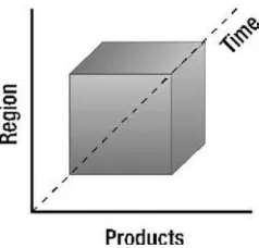
Data cubes are more sophisticated OLAP structures that will solve the preceding concern. Despite the name, cubes are not limited to a cube structure. The name is adopted just because cubes have more dimensions than rows and columns in tables. Don’t visualize cubes as only 3-dimensional or symmetric; cubes are used for their multidimensional value. For example, an airline company might want to summarize revenue data by flight, aircraft, route, and region. Flight, aircraft, route, and region in this case are dimensions. Hence, in this scenario, you have a 4-dimensional structure (a hypercube) at hand for analysis.
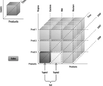
A simple cube can have only three dimensions, such as those shown in Figure 1-5, where X is Products, Y is Region, and Z is Time.
Table 1-1. OLTP vs. OLAP
Online Transaction Processing System
Online Analytical Processing System
Used for real-time data access.
Transaction-based.
Data might exist in more than one table.
Optimized for faster transactions.
Transactional databases include Add, Update, and Delete operations.
Not built for running complex queries.
Line-of-business (LOB) and
enterprise-resource-planning (ERP) databases use this model.
Tools: SQL Server Management Studio (SSMS).
Follows database (DB) normalization rules.
Relational database.
Holds key data.
Fewer indexes and more joins.
Query from multiple tables.
Used for online or historical data.
Used for analysis and drilling down into data.
Data might exist in more than one table.
Optimized for performance and details in querying the data.
Read-only database.
Built to run complex queries.
Analytical databases such as Cognos, Business Objects, and so on. use this model.
Tools: SQL Server Analysis Services (SSAS).
Relaxes DB normalization rules.
Relational database.
Holds key aggregated data.
Relatively more indexes and fewer joins.
With a cube like the one in Figure 1-5, you can find out product sales in a given timeframe. This cube uses Product Sales as facts with the Time dimension.
Facts (also called measures) and dimensions are integral parts of cubes. Data in cubes is accumulated as facts and aggregated against a dimension. A data cube is multidimensional and thus can deliver information based on any fact against any dimension in its hierarchy.
Dimensions can be described by their hierarchies, which are essentially parent-child relationships. If dimensions are key factors of cubes, hierarchies are key factors of dimensions. In the hierarchy of the Time dimension, for example, you might find Yearly, Half-Yearly, Quarterly, Monthly, Weekly, and Daily levels. These become the facts or members of the dimension.
In a similar vein, geography might be described like this:
Country
■
Dimensions, facts (or measures), and hierarchies together form the structure of a cube.
10
Now imagine cubes with multiple facts and dimensions, each dimension having its own hierarchies across each cube, and all these cubes connected together. The information residing inside this consolidated cube can deliver very useful, accurate, and aggregated information. You can drill down into the data of this cube to the lowest levels.
However, earlier we said that OLAP databases are denormalized. Well then, what happens to the tables? Are they not connected at all and just work independently?
Clearly, you must have the details of how your original tables are connected. If you want to convert your normalized OLTP tables into denormalized OLAP tables, you need to understand your existing tables and their normalized form in order to design the new mapping for these tables against the OLAP database tables you’re planning to create.
To plan for migrating OLTP to OLAP, you need to understand OLAP internals. OLAP structures its tables in its own style, yielding tables that are much cleaner and simpler. However, it’s actually the data that makes the tables clean and simple. To enable this simplicity, the tables are formed into a structure (or pattern) that can be depicted visually as a star. Let’s take a look at how this so-called star schema is formed and at the integral parts that make up the OLAP star schema.
Facts and Dimensions
OLAP data tables are arranged to form a star. Star schemas have two core concepts: facts and dimensions. Facts are values or calculations based on the data. They might be just numeric values. Here are some examples of facts:
Dell US Eastern Region Sales on Dec. 08, 2007 are $1.7 million. •
Dell US Northern Region Sales on Dec. 08, 2007 are $1.1 million. •
Average daily commuters in Loudoun County Transit in Jan. 2010 are 11,500. •
Average daily commuters in Loudoun County Transit in Feb. 2010 are 12,710. •
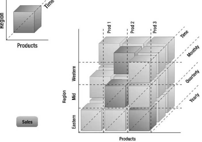
Dimensions are the axis points, or ways to view facts. For instance, using the multidimensional cube in Figure 1-6 (and assuming it relates to Wal-Mart), you can ask
What is Wal-Mart’s sales volume for Date mm/dd/yyyy? Date is a dimension. •
What is Wal-Mart’s sales volume in the Eastern Region? Region is a dimension. •
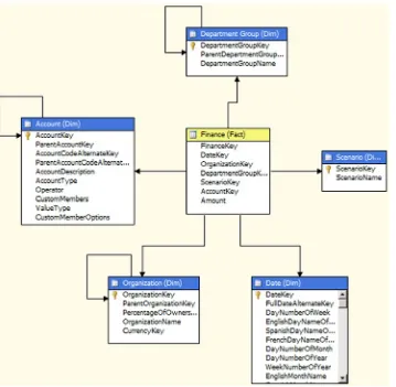
Values around the cube that belong to a dimension are known as members. In Figure 1-6, examples of members are Eastern (under the Region dimension), Prod 2 (under Products), and Yearly (under Time). You might want to aggregate various facts against various dimensions. Generating and obtaining a star schema is simple to do using SQL Server Management Studio (SSMS). You can create a new database diagram by adding more tables from the AdventureWorks database. SSMS will link related tables and form a star schema as shown in Figure 1-7.
Figure 1-7. A star schema
Note
■
OLAP and star schemas are sometimes spoken of interchangeably.
12
OLAP data is in the form of aggregations. You want to get from OLAP information such as the following:
The volume of sales for Wal-Mart last month •
The average salaries paid to employees this year •
A statistical comparison of your own company details historically, or a comparison against •
other companies
Note
■
Another model similar to the star schema is the snowflake schema, which is formed when one or more
dimension tables are joined to another dimension table (or tables) instead of a fact table. This results in reference
relationships between dimensions; in other words, they are normalized.
So far, so good! Although the OLAP system is designed with these schemas and structures, it’s still a relational database. It still has all the tables and relations of an OLTP database, which means that you might encounter performance issues when querying from these OLAP tables. This creates a bit of concern in aggregation.
Note
■
Aggregation is nothing but summing or adding data or information on a given dimension.
Extract, Transform, and Load
It is the structure of the cubes that solves those performance issues; cubes are very efficient and fast in providing information. The next question then is how to build these cubes and populate them with data. Needless to say, data is an essential part of your business and, as we’ve noted, typically exists in an OLTP database. What you need to do is retrieve this information from the OLTP database, clean it up, and transfer the data (either in its entirety or only what’s required) to the OLAP cubes. Such a process is known as Extract, Transform, and Load (ETL).
Note
■
ETL tools can extract information not only from OLTP databases, but also from different relational databases,
web services, file systems, or various other data sources.
You will learn about some ETL tools later in this chapter. We’ll start by taking a look at transferring data from an OLTP database to an OLAP database using ETL, at a very high level. But you can’t just jump right in and convert these systems. Be warned, ETL requires some preparation, so we’d better discuss that now.
Need for Staging
All of these common issues essentially demand an area where you can happily carry out all your operations—a staging or data-preparation platform. How would you take advantage of a staging environment? Here are the tasks you’d perform:
1. Identify the data sources, and prepare a data map for the existing (source) tables and entities.
2. Copy the data sources to the staging environment, or use a similar process to achieve this. This step essentially isolates the data from the original data source.
3. Identify the data source tables, their formats, the column types, and so on.
4. Prepare for common ground; that is, make sure mapping criteria are in sync with the destination database.
5. Remove unwanted columns.
6. Clean column values. You definitely don’t want unwanted information—just exactly enough to run the analysis.
7. Prepare, plan, and schedule for reloading the data from the source and going through the entire cycle of mapping.
8. Once you are ready, use proper ETL tools to migrate the data to the destination.
Transformation
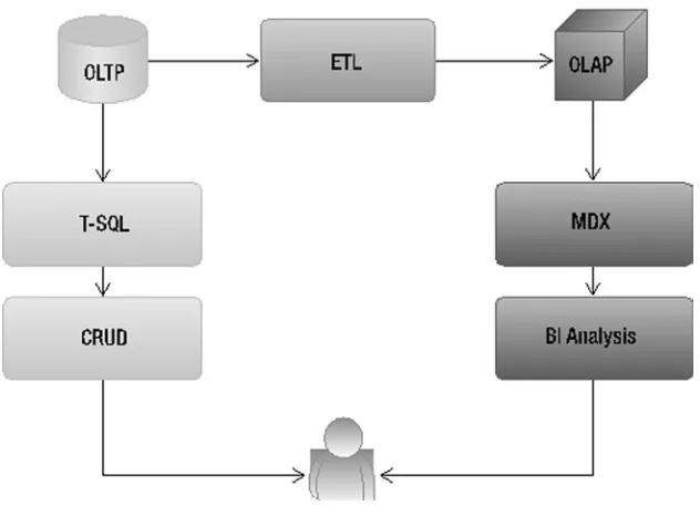
Let’s begin with a simple flow diagram, shown in Figure 1-8, which shows everything put together very simply. Think about the picture in terms of rows and columns. There are three rows (for system, language used, and purpose) and two columns (one for OLTP and the other for OLAP).
14
On OLTP databases, you use the T-SQL language to perform the transactions, while for OLAP databases you use MDX queries instead to parse the OLAP data structures (which, in this case, are cubes). And, finally, you use OLAP/MDX for BI analysis purposes.
What is ETL doing in Figure 1-8? As we noted, ETL is the process used to migrate an OLTP database to an OLAP database. Once the OLAP database is populated with the OLTP data, you use MDX queries and run them against the OLAP cubes to get what is needed (the analysis).
Now that you understand the transformation, let’s take a look at MDX scripting and see how you can use it to achieve your goals.
MDX Scripting
MDX stands for Multidimensional Expressions. It is an open standard used to query information from cubes. Here’s a simple MDX query (running on the AdventureWorks database):
select [Measures].[Internet Total Product Cost] ON COLUMNS, [Customer].[Country] ON ROWS
FROM [AdventureWorks]
WHERE [Sales Territory].[North America]
MDX can be a simple select statement as shown, which consists of the select query and choosing columns and rows, much like a traditional SQL select statement. In a nutshell, it’s like this:
Select x, y, z from cube where dimension equals a.
Sound familiar?
Let’s look at the MDX statement more closely. The query is retrieving information from the measure “Internet Total Product Cost” against the dimension “Customer Country” from the cube “AdventureWorks.” Furthermore, the
where clause is on the “Sales Territory” dimension, because you are interested in finding the sales in North America.
Note
■
Names for columns and rows are not case sensitive. Also, you can use 0 and 1 as ordinal positions for columns
and rows, respectively. If you extend the ordinal positions beyond 0 and 1, MDX will return the multidimensional cube.
MDX queries are not that different from SQL queries except that MDX is used to query an analysis cube. It has all the rich features, similar syntax, functions, support for calculations, and more. The difference is that SQL retrieves information from tables, resulting in a two-dimensional view. In contrast, MDX can query from a cube and deliver multidimensional views.
Go back and take a look at Figure 1-6, which shows sales (fact) against three dimensions: Product, Region, and Time. This means you can find the sales for a given product in a given region at a given time. This is simple. Now suppose you have regions splitting the US into Eastern, Mid and Western and the timeframe is further classified as Yearly, Quarterly, Monthly, and Weekly. All of these elements serve as filters, allowing you to retrieve the finest aggregated information about the product. Thus, a cube can range from a simple 3-dimensional one to a complex hierarchy where each dimension can have its own members or attributes or children. You need a clear understanding of these fundamentals to write efficient MDX queries.
In a multidimensional cube, you can either call the entire cube a cell or count each cube as one cell. A cell is built with dimensions and members.
Using our example cube, if you need to retrieve the sales value for a product, you’d do it as
Notice that square brackets—[ ]—are used when there’s a space in the dimension/member.
Looks easy, yes? But what if you need just a part of the cube value and not the whole thing? Let’s say you need just prod1 sales in the East region. Well that’s definitely a valid constraint. To address this, you use tuples in a cube.
Tuples and Sets
A tuple is an address within the cube. You can define a tuple based on what you need. It can have one or more dimensions and one measure as a logical group. For instance, if we use the same example, data related to the East region during the fourth quarter can be called one tuple. So the following is a good example of a tuple:
(Region.East, Time.[Quarter 4], Product.Prod1)
You can design as many as tuples you need within the limits of dimensions.
A set is a group of zero or more tuples. Remember that you can’t use the terms tuples and sets interchangeably. Suppose you want two different areas in a cube or two tuples with different measures and dimensions. That’s where you use a set. (See Figure 1-9.)
16
For example, if (Region.East, Time.[Quarter 4], Product.Prod1) is one of your tuples, and (Region.East, Time.[Quarter 1], Product.Prod2) is the second, then the set that comprises these two tuples looks like this:
{(Region.East, Time.[Quarter 4], Product.Prod1), (Region.East, Time.[Quarter 1], Product.Prod2)}
Best Practices
■
When you create MDX queries, it’s always good to include comments that provide sufficient
information and make logical sense. You can write single-line comments by using either “//” or “—” or multiline
comments using “/*…*/”.
For more about advanced MDX queries, built-in functions, and their references, consult the book Pro SQL Server 2012 BI
Solutions by Randal Root and Caryn Mason (Apress, 2012).
Putting It All Together
Table 1-2 gives an overview of the database models and their entities, their query languages, and the tools used to retrieve information from them.
Table 1-2. Database models
Nature of usage
Transactional (R/W)
Add, Update, Delete
Analytics (R)
Data Drilldown, Aggregation
Type of DB OLTP OLAP
Entities Tables, Stored Procedures, Views, and so on Cubes, Dimensions, Measures, and so on
Query Language(s) T-SQL/PL-SQL MDX
Tools SQL Server 2005 (or higher), SSMS SQL Server 2005 (or higher), SSMS, SSDT, SSAS
Before proceeding, let’s take a look at some more BI concepts.
The BI Foundation
Now that you understand OLAP system and cubes, let’s explore some more fundamental business intelligence (BI) concepts and terms in this section.
Data Warehouses
A data warehouse is a combination of cubes. It is how you structure enterprise data. Data warehouses are typically used at huge organizations for aggregating and analyzing their information.
Figure 1-10. Data warehouse and data marts
Data Marts
A data mart is a baby version of the data warehouse. It also has cubes embedded in it, but you can think of a data mart as a store on Main Street and a data warehouse as one of those huge, big-box shopping warehouses. Information from the data mart is consolidated and aggregated into the data-warehouse database. You have to regularly merge data from OLTP databases into your data warehouse on a schedule that meets your organization’s needs. This data is then extracted and sent to the data marts, which are designed to perform specific functions.
Note
■
Data marts can run independently and need not be a part of a data warehouse. They can be designed to
function as autonomous structures.
18
Decision Support Systems and Data Mining
Both decision support systems and data mining systems are built using OLAP. While a decision support system gives you the facts, data mining provides the information that leads to prediction. You definitely need both of these, because one lets you get accurate, up-to-date information and the other leads to questions that can provide intelligence for making future decisions. (See Figure 1-11.) For example, decision support provides accurate information such as “Dell stocks rose by 25 percent last year.” That’s precise information. Now if you pick up Dell’s sales numbers from the last four or five years, you can see the growth rate of Dell’s annual sales. Using these figures, you might predict what kind of sales Dell will have next year. That’s data mining.
Figure 1-11. Decision support system vs. data mining system
Note
■
Data mining leads to prediction. Prediction leads to planning. Planning leads to questions such as “What if?”
These are the questions that help you avoid failure. Just as you use MDX to query data from cubes, you can use the DMX
(Data Mining Extensions) language to query information from data-mining models in SSAS.
Tools
Now let’s get to some real-time tools. What you need are the following:
SQL Server Database Engine (Installation of the SQL Server 2012 will provision it) •
SQL Server Data Tools (formerly known as Business Intelligence Development Studio) •
AdventureWorks 2012 DW2012 sample database. •
Note
SQL Server Management Studio
SSMS is not something new to developers. You’ve probably used this tool in your day-to-day activities or at least for a considerable period during any development project. Whether you’re dealing with OLTP databases or OLAP, SSMS plays a significant role, and it provides a lot of the functionality to help developers connect with OLAP databases. Not only can you run T-SQL statements, you can also use SSMS to run MDX queries to extract data from the cubes.
SSMS makes it feasible to run various query models, such as the following:
• New Query: Executes T-SQL queries on an OLTP database
• Database Engine Query: Executes T-SQL, XQuery, and sqlcmd scripts • Analysis Services MDX Query: Executes MDX queries on an OLAP database • Analysis Services DMX Query: Executes DMX queries on an OLAP database
• Analysis Services XMLA Query: Executes XMLA language queries on an OLAP database Figure 1-12 shows that the menus for these queries can be accessed in SSMS.
Figure 1-12. Important menu items in SQL Server Management Studio
Note
■
The SQL Server Compact Edition (CE) code editor has been removed from SQL Server Management Studio in
SQL Server 2012. This means you cannot connect to and query a SQL CE database using management studio anymore.
TSQL editors in Microsoft Visual Studio 2010 Service Pack 1 can be used instead for connecting to a SQL CE database.
20
SQL Server Data Tools
While Visual Studio is the developer’s rapid application development tool, SQL Server Data Tools or SSDT (formerly known as Business Intelligence Development Studio or BIDS) is the equivalent development tool for the database developer. (See Figure 1-14.) SSDT looks like Visual Studio and supports the following set of templates, classified as Business Intelligence templates:
Analysis Services Templates •
• Analysis Services Multidimensional and Data Mining Project: The template used to create conventional cubes, measures, and dimensions, and other related objects
• Import from Server (Multidimensional and Data Mining): The template for creating an analysis services project based on a multidimensional analysis services database
• Analysis Services Tabular Project: Analysis service template to create Tabular Models, introduced with SQL Server 2012
• Import from PowerPivot: Allows creation of a Tabular Model project by extracting metadata and data from a PowerPivot for Excel workbook
• Import from Server (Tabular): The template for creating an analysis services Tabular Model project based on an existing analysis services tabular database
Integration Services Templates •
• Integration Services Project: The template used to perform ETL operations
• Integration Services Import Project Wizard: Wizard to import an existing integration services project from a deployment file or from an integration services catalog
Reporting Services Templates •
• Report Server Project Wizard: Wizard that facilitates the creation of reports from a data source and provides options to select various layouts and so on
• Report Server Project: The template for authoring and publishing reports
Figure 1-14. Creating a new project in SSDT
Transforming OLTP Data Using SSIS
As discussed earlier, data needs to be extracted from the OLTP databases, cleaned, and then loaded into OLAP in order to be used for business intelligence. You can use the SQL Server Integration Services (SSIS) tool to accomplish this. In this section, we will run through various steps detailing how to use Integration Services and how it can be used as an ETL tool.
SSIS is very powerful. You can use it to extract data from any source that includes a database, a flat file, or an XML file, and you can load that data into any other destination. In general, you have a source and a destination, and they can be completely different systems. A classic example of where to use SSIS is when companies merge and they have to move their databases from one system to another, which includes the complexity of having mismatches in the columns and so on. The beauty of SSIS is that it doesn’t have to use a SQL Server database.
Note
22
The important elements of SSIS packages are control flows, data flows, connection managers, and event handlers. (See Figure 1-15.) Let’s look at some of the features of SSIS in detail, and we’ll demonstrate how simple it is to import information from a source and export it to a destination.
Figure 1-15. SSIS project package creation
Because you will be working with the AdventureWorks database here, let’s pick some its tables, extract the data, and then import the data back to another database or a file system.
Open SQL Server Data Tools. From the File menu, choose New, and then select New Project. From the installed templates, choose Integration Services under Business Intelligence templates and select the Integration Services Project template. Provide the necessary details (such as Name, Location, and Solution Name), and click OK.
Once you create the new project, you’ll land on the Control Flow screen shown in Figure 1-15. When you create an SSIS package, you get a lot of tools in the toolbox pane, which is categorized by context based on the selected design window or views. There are four views: Control Flow, Data Flow, Event Handlers, and Package Explorer. Here we will discuss two main views, the Data Flow and the Control Flow:
Data Flow •
Data Flow Sources (for example, ADO.NET Source, to extract data from a database using •
a .NET provider; Excel Source, to extract data from an Excel workbook; Flat File Source, to extract data from flat files; and so on).
Data Flow Transformations (for example, Aggregate, to aggregate values in the dataset; •
Data Conversion, to convert columns to different data types and add columns to the dataset; Merge, to merge two sorted datasets; Merge Join, to merge two datasets using join; Multicast, to create copies of the dataset; and so on).
Data Flow Destinations (for example, ADO.NET destination, to write into a database using •
an ADO.NET provider; Excel Destination, to load data into a Excel workbook; SQL Server Destination, to load data into SQL Server database; and so on).
Based on the selected data flow tasks, event handlers can be built and executed in the •
Control Flow •
Control Flow Items (for example, Bulk Insert Task, to copy data from file to database; Data •
Flow Task, to move data from source to destination while performing ETL; Execute SQL Task, to execute SQL queries; Send Mail Task, to send email; and so on).
Maintenance Plan Tasks (for example, Back Up Database Task, to back up source database •
to destinations files or tapes; Execute T-SQL Statement Task, to run T-SQL scripts; Notify Operator Task, to notify SQL Server Agent operator; and so on).
Let’s see how to import data from a system and export it to another system. First launch the Import And Export Wizard from the Solution Explorer as shown in Figure 1-16. Then right-click on SSIS Packages and select the SSIS Import And Export Wizard option.
Figure 1-16. Using the SSIS Import and Export Wizard
Note
■
Another way to access the Import and Export Wizard is from
C:\Program Files\Microsoft SQL Server\110\DTS\Binn\DTSWizard.exe
.
Here are the steps to import from a source to a destination:
1. Click Next on the Welcome screen.
2. From the Choose a Data Source menu item, you can select various options, including Flat File Source. Select “SQL Server Native Client 11.0” in this case.
24
4. Use Windows Authentication/SQL Server Authentication.
5. Choose the source database. In this case, select the “AdventureWorks” database.
6. Next, choose the destination options and, in this case, select “Flat File Destination.”
7. Choose the destination file name, and set the format to “Delimited.”
8. Choose “Copy data from one or more tables or views” from the “Specify Table Copy or Query” window.
9. From the Flat File Destination window, click “Edit mappings,” leave the defaults “Create destination file,” and click OK.
10. Click Finish, and then click Finish again to complete the wizard.
11. Once execution is complete, you’ll see a summary displayed. Click Close. This step would create the .dtsx file, and you need to finally run the package once to get the output file.
Importing can also be done by using various data flow sources and writing custom event handlers. Let’s do it step by step in the next Problem Case.
PROBLEM CASE
Figure 1-17. Seven AdventureWorks sales tables
Here’s how to accomplish your goals:
1.
Open SSDT and, from the File menu, choose New. Then select New Project. From the
available project types, choose Integration Services (under Business Intelligence Projects),
and from the Templates choose Integration Services Project. Provide the necessary details
(such as Name, Location, and Solution Name), and click OK.
26
Clicking the link “No Data Flow tasks have been added to this package. Click here to add a new Data Flow task” (shown in Figure 1-18) enables the Data Flow task pane, where you can build a data flow by dragging and dropping the tool box items as shown in Figure 1-19. Add an ADO NET Source from the SSIS Toolbox to the Data Flow Task panel as shown in Figure 1-19.
Figure 1-18. Enabling the Data Flow Task panel
Figure 1-19. Adding a data flow source in SSIS
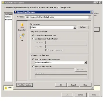
3.
Double-click ADO NET Source to launch the ADO.NET Source Editor dialog. Click the New
button to create a new Connection Manager.
4.
The list of data connections will be empty the first time. Click the New button again, and
connect to the server using one of the authentication models available.
Figure 1-21. SSIS Connection Manager data access mode settings Figure 1-20. SSIS Connection Manager
28
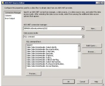
7.
Under “SQL command text,” enter a SQL query or use the Build Query option as shown
in Figure
1-22
. (Because I already prepared a script for this, that’s what I used. You’ll find
the SQL script ‘salesquery.txt’ in the resources available with this book.) Then click the
Preview button to view the data output.
Figure 1-22. ADONET Source Editor settings
9.
From the Data Flow Destinations section in the SSIS Toolbox, choose a destination that
meets your needs. For this demo, select Flat File Destination (under Other Destinations).
10.
Drag and drop Flat File Destination onto the Data Flow Task panel as shown in Figure
1-24
.
If you see a red circle with a cross mark on the flow controls, hover your pointer over the
cross mark to see the error.
30
11.
Connect the blue arrow from the ADO NET source to the Flat File Destination.
12.
Double-click on Flat File Destination, which opens the Editor. (See Figure
1-25
.)
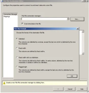
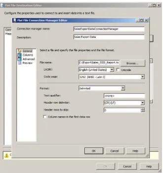
Figure 1-25. Flat File Format settings
13.
Click the New button to open the Flat File Format window, where you can choose among
several options. For this demo, select Delimited.
32
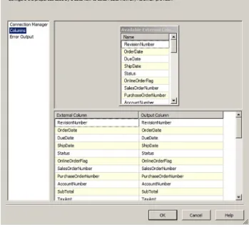
15.
On the next screen, click Mappings Node. Choose the Input Column and Destination
Columns and then click OK.
16.
The final data flow should look like Figure
1-27
.
Figure 1-27. SSIS Data Flow
17.
Start debugging by clicking F5, or click Ctrl+F5 to start without debugging.
18.
During the process, you’ll see the indicators (a circle displayed on the top right corner of
the Task) on data flow items change color to orange, with a rotating animation, indicating
that the task is in progress.
19.
Once the process completes successfully, the indicator on data flow items changes to
green (with a tick mark symbol), as shown in Figure
1-28
.
Figure 1-28. SSIS Data Flow completion
34
Figure 1-29. SSIS package execution progress
21.
Complete the processing of the package by clicking on Package Execution Completed
at the bottom of the package window.
22.
Now go to the destination folder and open the file to view the output.
23.
Notice that all the records (28,866) in this case are exported to the file and are
comma-separated.
Figure 1-30. SSIS data flow using the Aggregate transformation
Figure 1-31. SSIS data flow merge options
In many cases, you might actually get a flat file like this as input and want to extract it from and load it back into your new database or an existing destination database. In that scenario, you’ll have to take this file as the input source, identifying the columns based on the delimiter, and load it.
As mentioned before, you might have multiple data sources (such as two sorted datasets) that you want to merge. You can use the merge module and load the sources into one file or dataset, or any other destination, as shown in Figure 1-31.
Tip
36
Now let’s see how to move your OLTP tables into an OLAP star schema. Because you chose tables in the Sales module, let’s identify the key tables and data that need to be (or can be) analyzed. In a nutshell, you need to identify one fact table and other dimension tables first for the Sales Repository (as you see in Figure 1-32).
Figure 1-32. Sales fact and dimension tables in a star schema
The idea is to extract data from the OLTP database, clean it a bit, and then load it to the model shown in Figure 1-32. The first step is to create all the tables in the star schema fashion.
Table 1-3. Tables to create
Table Name
Column Name
Data Type
Key
Dim_Customer CustomerID Int, not null PK
AccountNumber Nvarchar(50), null
CustomerType Nvarchar(3), null
Dim_DateTime DateKey Int, not null PK
FullDate Date, not null
Dim_SalesOrderHeader SalesOrderHeaderID Int, not null PK
OrderDate Datetime, null
DueDate Datetime, null
Status Tinyint, null
Dim_SalesPerson SalesPersonID Int, not null PK, FK (to SalesPersonID in Dim_SalesTerritoryHistory,
TerritoryID Int, null FK (to TerritoryID in Dim_SalesTerritory table)
Dim_SalesTerritory TerritoryID Int, no null PK
38
Table Name
Column Name
Data Type
Key
Dim_SalesTerritoryHistory SalesTerritoryHistoryID Int, not null PK
SalesPersonID Int, not null FK (to SalesPersonID in Dim_SalesPerson table)
TerritoryID Int, not null FK (to TerritoryID in Dim_SalesTerritory table)
StartDate Date, null
EndDate Date, null
Dim_Store StoreID Int, not null PK
CustomerID Int, not null FK (to CustomerID in Dim_Customer table)
SalesPersonID Int, not null FK (to SalesPersonID in Dim_SalesPerson table)
Fact_SalesOrderDetails SalesOrderID Int, not null PK
SalesOrderHeaderID Int, not null FK (on SalesOrderHeaderID in Dim_SalesOrderHeader table)
DateKey Int, not null FK (to DateKey in Dim_DateTime table)
CustomerID Int, not null FK (to CustomerID in Dim_Customer table)
TerritoryID Int, not null FK (to TerritoryID in Dim_SalesTerritory table) Table 1-3. (continued)
Figure 1-33. Sample OLAP tables in a star schema
Notice the Fact_SalesOrderDetails table (fact table) and how it is connected in the star. And the rest of the tables are connected in the dimension model making up the star schema. There are other supporting tables, but we’ll ignore them for awhile because they might or might not contribute to the cube.
Note
40
You might be wondering how we arrived at the design of the tables.
Rule #1 when you create a schema targeting a cube is to identify what you would like to accomplish. In this case, we would like to know how Sales did with stores, territories, and customers, and across various date and time factors. (Recollect the cube in Figure 1-6.) Based on this, we identify the dimensions as Store, Territory, Date/Time, Customer, and Sales Order Header. Each of these dimensions will join to the Facts Table containing sales order details as facts.
As with the SSIS example you saw earlier (importing data from a database and exporting it to a flat file), you can now directly move the information into these newly generated tables instead of exporting it to the flat files.
One very important and useful data flow transformation is the Script Component, which you can use to
programmatically read the table and column values from the ADO NET Source (under the AdventureWorks database) and write to the appropriate destination tables (under the AdventureWorksDW database), using a script. While you do the extraction from the source, you have full control over the data and thus can filter the data, clean it up, and finally load it into the destination tables, making it a full ETL process. You simply drag and drop the Script Component from the Data Flow Transformations into the Data Flow, as shown in Figure 1-34.
Figure 1-34. Using the SSIS Script Component
Note
■
For more information on using the Script Component to create a destination, see the references at
msdn.microsoft.com/en-us/library/ms137640.aspx
and
msdn.microsoft.com/en-us/library/ms135939.aspx.
Tip
■
Many other operations—including FTP, e-mail, and connecting web services—can be accomplished using
SSIS. Another good real-time example of when you could use SSIS is when you need to import a text file generated from
another system or to import data into a different system. You can run these imports based on schedules.
Now that we’ve created the tables and transformed the data, let’s see how to group these tables in a cube, create dimensions, run an MDX query, and then see the results.
Creating Cubes Using SSAS
Microsoft SQL Server Analysis Services (SSAS) is a powerful tool you can use to create and process cubes. Let’s look at how cubes are designed, what the prerequisites are, and how cubes are created, processed, and queried using the MDX query language.
Note
■
SQL Server 2012 comes with a lot of new features. (Visit
msdn.microsoft.com/en-us/library/bb522628.aspxSSAS is used to build end-to-end analysis solutions for enterprise data. Because of its high performance and scalability, SSAS is widely used across organizations to scale their data cubes and tame their data warehouse models. Its rich tools give developers the power to perform various drill-down options over the data.
Let’s take care of the easy part first. One way to get started with cubes is by using the samples provided with the AdventureWorks database. You can download the samples from the msftdbprodsamples.codeplex.com/downloads/ get/258486 link. The download has two projects for both the Enterprise and Standard versions:
1. Open one of the folders based on your server license, and then open the AdventureWorks DW2012Multidimensional-EE.sln (for Enterprise Edition) file using SSDT.
2. Open the Project Properties and set the Deployment Target Server property to your SQL Server Analysis Services Instance.
3. Build and deploy the solution. If you get errors during deployment, use SQL Server Management Studio to check the database permissions. The account you specified for the data source connection must have a login on the SQL Server instance. Double-click the login to view the User Mapping properties. The account must have db_datareader permissions on the AdventureWorksDW2012 database.
This project contains lots of other resources, including data sources, views, cubes, and dimensions. However, these provide information relating to the layout, structure, properties, and so forth of SSDT, and they contain little information about cube structures themselves.
Once the project is deployed successfully (with no errors), open SSMS. You’ll find the cubes from the previous deployment available for access via MDX queries. Later in this chapter, you’ll learn how to create a simple cube. For now, we’ll use the available AdventureWorks cubes.
Executing an Analysis Services MDX query from SSMS involves few steps:
1. Run SQL Server Management Studio, and connect to the Analysis Services instance on your server by choosing Analysis Services under the Server type.
2. Click the New Query button, which launches the MDX Query Editor window.
3. In the MDX Query Editor window, from the Cube drop-down menu, select one of the available cubes from the Analysis Services database you’re connected to, “AdventureWorks” in this case.
4. Under the Metadata tab, you can view the various measures and dimensions available for the cube you selected.
5. Alternatively, you can click on the Analysis Services MDX Query icon at the top to open the query window.
6. Writing an MDX query is similar to writing a T-SQL query. However, instead of querying from tables, MDX queries from a cube’s measures and dimensions.
42
OK, so far you’ve seen the basic cube (using one from the AdventureWorks database) and also how to query from the cube using a simple MDX query. Let’s now begin a simple exercise to build a cube from scratch.
Using data from the Sales Repository example you saw earlier, let’s configure a cube using the Dimension and Fact tables you created manually with the AdventureWorksDW database:
1. Once you have the data from SSIS in the designated tables (structured earlier in this chapter), you can create a new project under SSAS.
2. Open SSDT, and create a New Project by selecting Analysis Services Multidimensional and Data Mining Project.
3. Provide a valid project name, such as AW Sales Data Project, a Location, and a Solution Name. Click OK.
4. A basic project structure is created from the template, as you can see in Figure 1-36. Figure 1-35. Executing a simple MDX query
5. Create a new data source by right-clicking on Data Sources and selecting New Data Source; this opens the New Data Source Wizard.
6. Click the New button, and choose the various Connection Manager options to create the new Data Connection using the database AdventureWorksDW2012.
7. Click Next, and choose “Use the service account” for the Impersonation option. You can also choose other options based on how your SQL Server is configured.
8. Click Next, provide a valid Data Source Name (AW Sales Data DW in this case), and click Finish, as shown in Figure 1-37.
Figure 1-37. The SSAS Data Source Wizard completion screen
The next step is to create the data source views, which are important because they provide the necessary tables to create the dimensions. Moreover, a view is the disconnected mode of the database; hence, it won’t have any impact on performance.
9. Right-click Data Source Views, and choose New Data Source View, which brings up the Data Source View Wizard.
10. Select an available data source. You should see the AW Sales Data DW source you just created.
44
12. To save the data source view, provide a valid name (AW Sales Data View) and click Finish.
13. Notice that Design View now provides a database diagram showing all the tables selected and the relations between each of them.
14. Now you can create either a dimension or a cube, but it’s always preferable to create dimensions first and then the cube, because the cube needs the dimensions to be ready. Right-click Dimensions, and choose New Dimension, which brings up the Dimension Wizard.
15. Click Next. On the Select Creation Method screen, choose “Use an existing table” to create the dimension source, and then click Next.
16. On the next screen, choose the available Data source view. For the Main table, select Dim_DateTime and then click Next.
17. The next screen displays the available attributes and types. (See Figure 1-39.) Notice the attribute types that are labeled “Regular.” By default, only the primary keys of the tables are selected in the attributes for each dimension. You need to manually select the other attributes. This step is important because these are the values you query in MDX along with the available measures.
18. Choose the attributes Month Name, Quarter, and Year in our sample, and change the attribute types to Month, Quarter, and Year, respectively, as shown in Figure 1-39. Click Next.
19. Provide a logical name for the dimension (Dim_Date in our case), and click Finish. This creates the Dim_Date.dim dimension in the Dimensions folder in your project.
20. In Solutions Explorer, right-click the Cubes folder and choose New Cube to bring up the Cube Wizard welcome screen. Click Next.
21. On the Select Creation Method screen, choose “Use existing tables” and then click Next.
22. From the available “Measure group tables” list, select the fact table or click the Suggest button. (See Figure 1-40.)
46
23. If you choose Suggest, the wizard selects the available measure group tables. You can choose your own Measure Group tables in the other case. Click Next to continue.
24. The Select Measures screen displays the available measures, from which you can either select all or just what you need. Leave the default to select all, and click Next to continue.
25. Now you can choose to Select Existing Dimensions from any available. For now, you can leave the default—the existing dimension. Click Next to continue.
26. The Select New Dimensions screen gives you the option to choose new dimensions that the wizard identifies from the data source selected. If you already chose a dimension in the previous step, ignore that dimension or just click Next to continue. If you previously created a dimension and also selected the same one that’s listed here, the wizard creates another dimension with a different name. Click Next.
27. Provide a valid cube name, AW Sales Data View, as shown in Figure 1-41. Notice that Preview displays all the measures and dimensions chosen for this cube. Click Finish to complete the step.
48
29. In the Dimensions window (usually found in the bottom left corner), expand each of the dimensions and notice that the attributes are just the primary key columns of the table. (See Figure 1-43.) You need all the attributes or at least the important columns you want to run analyses on.
30. From the Dimensions folder in Solution Explorer, double-click each of the dimensions to open the Dimension Structure window (shown in Figure 1-44).
Figure 1-43. SSAS project dimension settings
Figure 1-44. The Dimension Structure screen showing Attributes, Hierarchies, and Data Dource View
50
32. Repeat the same steps for the rest of the dimensions, and click Save All. Refresh the window, and notice that all columns now appear under attributes and have been added to the Dimensions.
33. To add hierarchies, drag and drop the attribute or attributes from the Attributes pane to the Hierarchies pane. Repeat the step for all of the dimensions. When you’re done, go back to the Cube Structure window.
34. On the left in the Measures pane, you now have only one measure—Fact Sales Order Details Count. To create more measures, simply right-click on the Measures window and choose New Measure.
35. From the New Measure dialog box, select the option “Show all columns.”
36. For the Usage option, select Sum as the aggregation function. Then choose
Dim_SalesTerritory as the Source Table and SalesYTD as Source Column, and click OK. This provides a new measure, Sales YTD, by summing the values from a given territory against the available dimensions.
37. All is well at this time. Your final window looks something like what’s shown in Figure 1-45.
Figure 1-45. The AW Sales Data Project sample
39. This step builds and deploys the project to the target server. You can view the deployment status and output in the deployment progress window.
40. If the deployment is successful, you’ll see a “Deployment Completed Successfully” message at the bottom of the progress window, as shown in Figure 1-46.
Figure 1-46. The Deployment Progress window
41. Let’s now switch applications and open SSMS.
52
43. Object Explorer displays the available databases. You’ll find the AW Sales Data Project you created earlier in BIDS and deployed locally. Expand the options, and notice the various entities available under the Data Sources, Data Source Views, Cubes, and Dimensions (See Figure 1-48.)
Figure 1-48. BIDS databases
44. Click the MDX Query icon on the toolbar to open the query window and the cube window. Make sure the appropriate data source is selected at the top.
45. The cube will display the available Measures and Dimensions, as shown in Figure 1-49.
Figure 1-49. Running a simple MDX query
46. In the query window, type the MDX query to retrieve the values from the cube. In this case, to get the Sum of Sales YTD in the Sales Territory Measure, the query should look like the one in Figure 1-49.
47. Execute and parse the query to view the output in the results window.
Final Pointers for Migrating OLTP Data to OLAP
Now that you know the concepts, let’s see some of the important factors to keep in mind while planning for a migration. First, you need to be completely aware of why you need to migrate to an OLAP database from an OLTP database. If you are not clear, it’s a good idea to go back to the section “Online Analytical Processing System” and make a checklist (and also review the need for a staging section). Be sure to consider the following items:
Make sure that there is no mismatch in column names between the two ends. Most of •
the time, you don’t have same columns anyway; in such cases, maintain metadata for the mapping. ETL tools (in this case, SSIS) support different column names.
While mapping columns between the source and destination, there is a good possibility that •
the data types of the columns might not match. You need to ensure that type conversion is taken care of during transformation.
With OLAP, the idea is to restrict the number of columns and tables and denormalize as much •