Getting Started with RStudio
John Verzani
Getting Started with RStudio by John Verzani
Copyright © 2011 John Verzani. All rights reserved. Printed in the United States of America.
Published by O’Reilly Media, Inc., 1005 Gravenstein Highway North, Sebastopol, CA 95472.
O’Reilly books may be purchased for educational, business, or sales promotional use. Online editions are also available for most titles (http://my.safaribooksonline.com). For more information, contact our corporate/institutional sales department: (800) 998-9938 or [email protected].
Editor: Mike Loukides Production Editor: Kristen Borg
Proofreader: O’Reilly Production Services
Cover Designer: Karen Montgomery Interior Designer: David Futato Illustrator: Robert Romano
Nutshell Handbook, the Nutshell Handbook logo, and the O’Reilly logo are registered trademarks of O’Reilly Media, Inc. Getting Started with RStudio, the image of a ribbonfish, and related trade dress are trademarks of O’Reilly Media, Inc.
Many of the designations used by manufacturers and sellers to distinguish their products are claimed as trademarks. Where those designations appear in this book, and O’Reilly Media, Inc., was aware of a trademark claim, the designations have been printed in caps or initial caps.
While every precaution has been taken in the preparation of this book, the publisher and authors assume no responsibility for errors or omissions, or for damages resulting from the use of the information con-tained herein.
Table of Contents
Using the Right Class to Store Data 19
Data Cleaning 20
Using the Code Editor to Write R Scripts 21
Using Add-On Packages 22
Graphics 23
Command History 24
All Finished, for Now 25
Preface
Conventions Used in This Book
The following typographical conventions are used in this book:
Italic
Indicates new terms, URLs, email addresses, filenames, and file extensions. Constant width
Used for program listings, as well as within paragraphs to refer to program elements such as variable or function names, databases, data types, environment variables, statements, and keywords.
Constant width bold
Shows commands or other text that should be typed literally by the user.
Constant width italic
Shows text that should be replaced with user-supplied values or by values deter-mined by context.
This icon signifies a tip, suggestion, or general note.
This icon indicates a warning or caution.
Using Code Examples
This book is here to help you get your job done. In general, you may use the code in this book in your programs and documentation. You do not need to contact us for permission unless you’re reproducing a significant portion of the code. For example, writing a program that uses several chunks of code from this book does not require permission. Selling or distributing a CD-ROM of examples from O’Reilly books does require permission. Answering a question by citing this book and quoting example code does not require permission. Incorporating a significant amount of example code from this book into your product’s documentation does require permission.
We appreciate, but do not require, attribution. An attribution usually includes the title, author, publisher, and ISBN. For example: “Getting Started with RStudio by John Ver-zani (O'Reilly). Copyright 2011 John VerVer-zani, 978-1-449-30903-9.”
If you feel your use of code examples falls outside fair use or the permission given above, feel free to contact us at [email protected].
Safari® Books Online
Safari Books Online is an on-demand digital library that lets you easily search over 7,500 technology and creative reference books and videos to find the answers you need quickly.
With a subscription, you can read any page and watch any video from our library online. Read books on your cell phone and mobile devices. Access new titles before they are available for print, and get exclusive access to manuscripts in development and post feedback for the authors. Copy and paste code samples, organize your favorites, down-load chapters, bookmark key sections, create notes, print out pages, and benefit from tons of other time-saving features.
O’Reilly Media has uploaded this book to the Safari Books Online service. To have full digital access to this book and others on similar topics from O’Reilly and other pub-lishers, sign up for free at http://my.safaribooksonline.com.
How to Contact Us
Please address comments and questions concerning this book to the publisher: O’Reilly Media, Inc.
1005 Gravenstein Highway North Sebastopol, CA 95472
800-998-9938 (in the United States or Canada) 707-829-0515 (international or local)
We have a web page for this book, where we list errata, examples, and any additional information. You can access this page at:
http://shop.oreilly.com/product/0636920021278.do
To comment or ask technical questions about this book, send email to:
For more information about our books, courses, conferences, and news, see our website at http://www.oreilly.com.
Find us on Facebook: http://facebook.com/oreilly
Follow us on Twitter: http://twitter.com/oreillymedia
Watch us on YouTube: http://www.youtube.com/oreillymedia
CHAPTER 1
Overview, Installation
This book introduces users to the RStudio Integrated Development Environment (IDE) for using and programming R, the widely used opsource statistical computing en-vironment. RStudio is a separate open-source project that brings many powerful coding tools together into an intuitive, easy-to-learn interface. RStudio runs in all major plat-forms (Windows, Mac, Linux) and through a web browser (using the server installa-tion). This book should appeal to newer R users, students who want to explore the interface to get the most out of R, and long-time R users looking for a more modern development environment.
RStudio is periodically released as a stable version, and has daily releases in between. This book, as written, describes one of the daily releases—in particular, version 0.95.75; the current stable release is version 0.94.102. Some features described here, such as the project feature, are not currently available in the stable release.
We will begin with a quick overview of R and IDEs before diving into RStudio.
What is R?
R is an open-source software environment for statistical computing and graphics. R compiles and runs on Windows, Mac OS X, and numerous UNIX platforms (such as Linux). For most platforms, R is distributed in binary format for ease of installation. The R software project was first started by Robert Gentleman and Ross Ihaka. The language was very much influenced by the S language, which was originally developed at Bell Laboratories by John Chambers and colleagues. Since then, with the direction and talents of R’s core development team, R has evolved into the lingua franca for statistical computations in many disciplines of academia and various industries. R is much more than just its core language. It has a worldwide repository system, the
Comprehensive R Archive Network (CRAN)—http://cran.r-project.org—for
user-contributed add-on packages to supplement the base distribution. As of 2011, there were more than 3,000 such packages hosted on CRAN and numerous more on other
sites. In total, R currently has functionality to address an enormous range of problems and still has room to grow.
R is designed around its core scripting language but also allows integration with com-piled code written in C, C++, Fortran, Java, etc., for computationally intensive tasks or for leveraging tools provided for other languages.
What is an IDE?
R, like other programming languages, is extended (or developed) through user-written functions. An integrated development environment (IDE), such as RStudio, is designed to facilitate such work. In addition, unlike many other statistical software packages in which a graphical user interface is employed, a typical user interacts with R primarily through the command line. An IDE for R then must also include a means for issuing commands interactively. R is not unique in this respect, and IDEs for interactive sci-entific programming languages have matured to include features such as:
• A console for issuing commands.
• Source-code editor; at its core, development involves the act of programming, and this task is inevitably done with a source-code editor. Such editors have been around for some time now, and expectations for editors are now quite demanding. A typical set of expectations includes:
— A rich set of keyboard shortcuts
— Automatic source-code formatting, assistance with parentheses, keyword highlighting
— Code folding and easy navigation through a file and among files — Context-sensitive assistance
— Interfaces for compiling or running of software — Project-management features
— Debugging assistance
— Integration with report-writing tools
• Object browsers; in interactive use, a user’s workspace includes variables that have been defined. An object browser allows the user to identify quickly the type and values for each such variable.
• Object editors; from an object browser, a means to inspect or edit objects is typi-cally provided.
• Integration with the underlying documentation. • Plot-management tools.
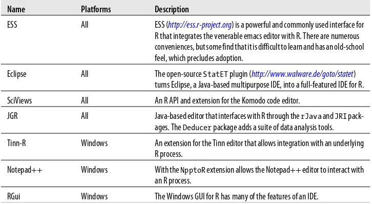
Table 1-1. Some existing IDEs for R
Name Platforms Description
ESS All ESS (http://ess.r-project.org) is a powerful and commonly used interface for R that integrates the venerable emacs editor with R. There are numerous conveniences, but some find that it is difficult to learn and has an old-school feel, which precludes adoption.
Eclipse All The open-source StatET plugin (http://www.walware.de/goto/statet) turns Eclipse, a Java-based multipurpose IDE, into a full-featured IDE for R.
SciViews All An R API and extension for the Komodo code editor.
JGR All Java-based editor that interfaces with R through the rJava and JRI pack-ages. The Deducer package adds a suite of data analysis tools.
Tinn-R Windows An extension for the Tinn editor that allows integration with an underlying R process.
Notepad++ Windows With the NpptoR extension allows the Notepad++ editor to interact with an R process.
RGui Windows The Windows GUI for R has many of the features of an IDE.
Why RStudio?
The RStudio project currently provides most of the desired features for an IDE in a novel way, making it easier and more productive to use R. Some highlights are:
• The main components of an IDE are all nicely integrated into a four-panel layout that includes a console for interactive R sessions, a tabbed source-code editor to organize a project’s files, and panels with notebooks to organize less central components.
• The source-code editor is feature-rich and integrated with the built-in console. • The console and source-code editor are tightly linked to R’s internal help system
through tab completion and the help page viewer component.
• Setting up different projects is a snap, and switching between them is even easier. • RStudio provides many convenient and easy-to-use administrative tools for
man-aging packages, the workspace, files, and more.
• The IDE is available for the three main operating systems and can be run through a web browser for remote access.
• RStudio is much easier to learn than Emacs/ESS, easier to configure and install than Eclipse/StatET, has a much better editor than JGR, is better organized than Sciviews, and unlike Notepad++ and RGui, is available on more platforms than just Windows.
The RStudio program can be run on the desktop or through a web browser. The desktop version is available for Windows, Mac OS X, and Linux platforms and behaves similarly across all platforms, with minor differences for keyboard shortcuts.
To achieve this cross-platformness, RStudio leverages numerous existing web technol-ogies in its design. For the desktop applications, it cleverly displays them within an
industry standard HTML widget provided by Qt (a cross-platform application and UI
framework) to create a desktop application. Consequently, R users can have a feature-rich and consistent programming environment for R their way—desktop- or web-based. Web-based usage is not in the “cloud” (although that service may be forthcom-ing), but rather can be done through a trusted server within a department or organi-zation.
RStudio is the brainchild of J. J. Allaire, who, with his brother, previously had tremen-dous success developing the influential ColdFusion IDE and scripting language for web development. Allaire is currently joined by the very able Joseph Cheng, Joshua Paulson, and Paul DiCristina. In the short time that their initial beta has been available, they have proven to be very responsive to user input. RStudio is under active development. As such, elements discussed in this book may be changed by the time you are reading it. Sorry…but you’ll likely be better off with the new feature than my description of the old one.
Like R, RStudio is an open-source project. Its stated goal—which it is already meeting —is to develop a powerful tool that supports the practices and techniques required for creating trustworthy, high-quality analysis. The codebase is released under the AGPLv3 license and is available from GitHub (https://github.com/rstudio/rstudio). RStudio is built on top of many other open-source projects. Most visible of these are GWT, Goo-gle’s Web Toolkit; Qt, the graphical toolkit of Nokia; and Ace, the JavaScript code editor (http://ace.ajax.org). Other leveraged projects are listed in RStudio’s About dialog. The bulk of the code is written in C++ and Java, the language for working with GWT.
Using RStudio
We will reverse things slightly by beginning with the process of starting RStudio, and postpone any installation issues for a bit. As RStudio can be used from the desktop or through a server, there are two ways of starting it.
Desktop Version
For the desktop version, RStudio is started like most other applications. In Fig-ure 1-1, we see the application running under Mac OS X. There it was started by clicking on its icon in the Applications folder. For Windows users, the installation process
leaves a menu item. For Linux users, the command rstudio will open the window. It
In Figure 1-1 we see three main components: the Console, which should look familiar to any R user; a Workspace browser (with no items, as the initial workspace is empty) and the History interface. The latter two are part of notebooks that contain other
com-ponents. The Source component, or code editor, is not open in the screenshot, as no
files are open for editing or viewing.
Server Version
Starting the server version requires one to know the appropriate URL for the resource. We used a local URL for this book, but the real value comes from using RStudio as a resource on the wider internet. When accessing RStudio, one must first authenticate. The basic screen to do so looks like Figure 1-2. Authentication depends on the server, but the default is to authenticate against the user accounts on the machine, so the web adminstrator should have provided a secure means to access RStudio.
Once authenticated, the layout looks similar to that of the desktop version—compare
Figure 1-1 to Figure 1-3 to see this. One main difference is the location of the menu bar. In the desktop figure, under Mac OS X, the menu bar is placed following the custom of that operating system—detached from the application and at the top of the screen —and is not integrated into the RStudio GUI. For the server version, the menu bar appears above the application’s main toolbar.
Figure 1-1. RStudio on initial startup; the main interface has four panels (one hidden in this screenshot), a toolbar, and in some cases, a menu bar
When using the server version, only one instance per user may be opened. If a new session is started—on a different machine, or even if just in a different tab of the same browser—the old one is disconnected and a notification issued.
Figure 1-2. Login screen for the server version of RStudio
Which Workspace?
When R is started, it follows this process: • R is started in the working directory.
• If present, the .Rprofile file’s commands are executed. • If present, the .Rdata file is loaded.
• Other actions described in ?Startup are followed.
When R quits, a user is queried to “Save workspace image?” When the workspace is saved it writes the contents to an .Rdata file, so that when R is restarted the workspace can persist between sessions. (One can also initiate this with save.image.)
This process allows R users to place commands they desire to run in every session in an .Rprofile file, and to have per directory .Rdata files, so that different global work-spaces can be used for different projects.
Projects
RStudio provides a very useful “project” feature that allows a user to switch quickly between projects. Each project may have different working directories, workspaces, and collection of files in the Source component. The current project name is listed on the far right of the main application toolbar in a combobox that allows one to switch between open projects, open an existing project, or create a new project.
A new project requires just a name and a working directory. This feature is a natural fit for RStudio, because when it runs as a web application, there is a need to serialize and restore sessions due to the nature of web connections. Switching between projects is as easy as selecting an open project. RStudio just serializes the old one and restores the newly selected one.
As of writing, the “project” feature is not available in the stable release (0.94.102) but is in the “daily build” version.
Which R?
RStudio does not require a special version of R to run, as long as it is a fairly modern one. It will work with binary versions from CRAN or user-compiled versions. As such, when RStudio starts up, it must be able to locate a version of R, which could possibly reside in many different places. Usually RStudio just finds the right one, but one can bypass the search process. The document online at http://www.rstudio.org/docs/ad-vanced/versions_of_r details how to specify which R installation to use. In short, it depends on the underlying operating system. For Windows desktop users, it can be
specified in the Options dialog (“The Options Dialog” on page 9). For Linux and Mac OS X users, one can set an environment variable, as seen here:
$ export RSTUDIO_WHICH_R=/usr/local/bin/R
Web-based users really don’t have a choice, as this is determined by who configures the server.
Layout of the Components
The RStudio interface consists of several main components sitting below a top-level toolbar and menu bar. Although this placement can be adjusted, the default layout utilizes four main panels or panes in the following positions:
• In the upper left is a Source browser notebook for editing files (see “Source Code
Editor” on page 63) or viewing some data sets. In Figure 1-3 this is not visible, as that session had no files open.
• In the lower left is a Console for interacting with an R process (Chapter 3). • In the upper right is a notebook widget to hold a Workspace browser (“Workspace
Browser” on page 38) and History browser (“Command History” on page 36). • In the lower right is a notebook to hold tabs for interacting with the Files (“The
File Browser” on page 71), Plots (“The Browser” on page 45), Packages (“Package Maintenance” on page 73), and Help system components (“The Help Page Viewer” on page 42).
The Console pane is somewhat privileged: it is always visible, and it has a title bar. The other components utilize notebook widgets, and the page tabs serve as a title bar. These pages have page-specific toolbars (perhaps more than one)—which in the case of the Source component are also context-specific.
The user may change the default allocation of space for each of the panes. There is a sash appearing in the middle of the interface between the left and right sides that allows the user to adjust the horizontal allocation of space. Furthermore, each side then has another sash to allocate the vertical space between its two panes. As well, the title bar of each pane has icons to shade a component, maximize a component vertically, or share the space.
Keyboard Shortcuts
One can easily switch between components using the mouse. As well, the View menu
bar has subitems for this task. For power users, the keyboard accelerators listed in
Table 1-2. Keyboard shortcuts for navigation between major components
Description Windows & Linux Mac
Move cursor to Source Editor Ctrl+1 Ctrl+1
Move cursor to Console Ctrl+2 Ctrl+2
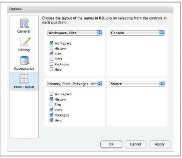
RStudio preferences are adjusted through the Options dialog . There are four panels for this dialog to adjust: general properties, editing properties (Figure 3-4), appearance properties and pane layout (Figure 1-4).
The pane layout allows the user to determine which panes go in which corners, and, for the supplemental components (not the Console or Source editor), which compo-nents are rendered in which notebook. One modifies a placement simply by adjusting a combobox, or by checking one of the checkboxes. In Figure 1-4, the choices put the code editor on the right, the console in the lower right, and the file browser on the
upper left. There are many examples of panel placement on
http://rstudio.org/screen-shots/.
The appearance panel of the options dialog allows one to set the default font size and modify the theme for the editing in the console or source-code editor. This book uses the default TextMate theme for its screenshots.
Installing RStudio
Installing RStudio is usually a straightforward process.
First, RStudio requires a working, relatively modern R installation. If that is not already present, then one should consult http://cran.r-project.org to learn how to install R for the given operating system. For Windows and Mac OS X, one can simply download a self-installing binary; for Linux, installation varies. For the Debian distribution (in-cluding Ubuntu), the R system can be installed using the regular package-management tools. Of course, as R is open source, one can also compile and install it using the source code.
The RStudio package is available for download from http://www.rstudio.org/down-load/. There is a choice between a Desktop version and a Server version. The Desktop version is appropriate for single-user use. The files come in a common format for binary installation (e.g., exe, dmg, deb, or rpm). One downloads the file and installs it as any other program.
For those searching out the latest features, follow the link on http://www.rstudio.org/ download/daily to get the binaries for the most recent (but not necessarily stable) build. Installing a server version requires more work and care. Some directions are given at
http://rstudio.org/docs/.
One can also install RStudio from its source code. A link for the source “tarball” for the current stable version appears on the appropriate download page. For the adven-turous, the latest development build files are available from https://github.com/rstudio/ rstudio. Installation details are in the INSTALL file accompanying the source code. The same source is used to compile both the Desktop and Server version.
As RStudio depends on some of the latest features of many moving parts, such as GWT,
there can be issues with compiling from the source. The support forums (
http://sup-port.rstudio.org/) are an excellent place to find specific answers to any issues.
Logging
RStudio creates secret files for itself to store information, including log-ging information. When there are issues at startup, the log can be con-sulted for direction as to what is going wrong.
For desktop users, the log directory is either ~/.rstudio-desktop/log for Mac and Linux users; or for Windows users, %localappdata%\RStudio-Desktop\log (Windows Vista and 7) or %USERPROFILE%\Local Set-tings\Application Data\RStudio-Desktop\log for XP.
In the application’s menu bar, the Help > Diagnostics item can be used to find the log files.
Updating RStudio
Updating RStudio is also straightforward.
To see if an update is available, the Help > Check for Updates menu item will open a dialog with update information.
If an update is available, one can stop RStudio, install the new version, then restart. RStudio writes session information to the user’s home directory (e.g., to the file ~/.rstu-dio-desktop). This will persist between upgrades.
CHAPTER 2
Case Study: Data Cleaning
Now that we know how to start RStudio, let’s dive in. We’ll begin with a blow-by-blow account of a sample data analysis for which we read in some data, clean it up, then format it for further study. The point of the exercise is to show how many of RStudio’s features can be used during the process to speed the task along. We will postpone for now an example of the “development” aspect of RStudio.
The data set we look at here comes from a colleague, and contains records from a psychology experiment on a colony of naked mole rats. The experimenter is interested in both the behavior of each naked mole rat in time and the social aspect of the colony as a whole.
Each rat wears an RFID chip that allows the researcher to track its motion. The ex-periment consists of 15 chambers (bubbles) in a linear arrangement separated by 14 tubes. Each tube has a gate with a sensor. When a mole rat passes through the tube, the time and gate are recorded. Unfortunately, gates can be missed, and the recording device can erroneously replicate values, so the raw data must be cleaned up.
This data comes to us in rich-text format (rtf). This quasi text-based format is a bit unusual for data transfer but presumably is used by the recording apparatus. We will see that this format has some idiosyncrasies that will require us to work a little harder than we might normally do to read data into an RStudio session, but don’t worry, RStudio is up to the task.
Our first step is to copy the file into a directory named NMR. We are performing this analysis using the desktop version, so we simply copy files the usual way after making a new directory. Had we been working through a server, we could have uploaded the file into a new directory using first the New Folder toolbar button, then the Upload toolbar button of the Files component.
Using Projects
To organize our work, we set up a new project. RStudio allows us to compartmentalize our work into projects that have separate global workspaces and associated files. We easily navigate between projects using a selector (a combobox) in the main toolbar located in the upper-right corner. The same selector has an option to create a New Project..., which we choose. To create a new project, one fills in a project name and location.
When the project is created, the working directory is set. The title bar of the Console panel is updated, as are the contents of the Files component, which lists the files and subdirectories in a given directory. The Files component resides in a notebook, which by default is placed in the upper-right corner. If it isn’t showing, select its tab. In
Figure 2-1, we see that our working directory contains our data file and a bookkeeping file that RStudio created.
Figure 2-1. The Files browser shows files added when a new project is created
The Files browser panel is typical of RStudio’s components. In addition to the main application toolbar, most components come with their own toolbar. In this case, the toolbar has buttons to add a new folder, delete selected files, etc. In addition, the Files component adds a second toolbar to facilitate the selection of files and navigation within directories.
Reading in a Data File
Clicking on the data file name in the file browser opens up a system text editor ( Fig-ure 2-2), allowing us to edit the file. For many text-based files, the file will open in RStudio’s source-code editor. However, the actual editor employed depends on the extension and MIME type of the file. For rtf files, the underlying operating system’s
editor is used, which for Mac OS X is textedit. We can see that the data appears to
date, time, and gate number. This is basically comma-separated-value (CSV) data with a nonstandard separator.
However, although we rarely see rtf files, we know the textedit program will likely render them using the markup for formatting, so perhaps there are some markup com-mands that needs to be removed. To investigate, we make a copy of the data file, but store it instead with a txt extension. The Files component makes it easy to perform basic file operations such as this. To make a copy of a file, one selects the checkbox next to the file and invokes the More > Copy… menu item, as seen in Figure 2-3.
Figure 2-3. Copying files in the Files browser—the command acts on the checked file
We change the extension to txt and our file list is updated. The displayed contents of the directory may also be refreshed by clicking the terminus on the path indicated by the links to the right of the house icon in the secondary toolbar; or the curved arrow icon on the far right of the component’s main toolbar. Now, clicking on the txt file opens the file in RStudio’s source-code editor as a text file (Figure 2-4).
Figure 2-2. The rtf file is opened in an editor provided by the system, not by RStudio
The editor’s status bar shows us the line and position of the cursor and, on the far right, that we are looking at a text file. We can now see that there is indeed a header (and, if we scroll down, a footer) wrapping our data. We highlight the header and then use the Delete key to remove this content from the file. We then scroll to the bottom of the file and remove a trailing brace. Afterwards, we click the Save toolbar button (the upper-left toolbar button, which is grayed out in the figure, as no changes have been made).
We now wish to read in the file using read.csv. RStudio provides an Import Dataset
toolbar button under the Workspace component, which provides an interface that will
handle most csv data, such as that exported from a spreadsheet. In this example though, we have a few idiosyncrasies that prevent its use. (This is a deliberate choice to show off some of RStudio’s other features.)
So we head on over to the Console component to do the work. With the default panel
arrangement the console is located on the left side, usually in the lower-left panel. In R, one can’t avoid the console, and RStudio’s should look very familiar.
Tab Key Completion
At the console we create the command to call the function directly. This requires us to specify a few of its arguments, as we have a different separator, an odd character every other line, and no header. We will use the tab completion feature to assist us in filling in these values. This feature provides completion candidates for many different settings, allowing us in this case to recall quickly the names for lesser-used arguments.
First, we type read.csv in the console. Then we press the Tab key to bring up the tab completion dialog (Figure 2-5) for this function.
Figure 2-5. Tab-key completion dialog showing small snippet about the read.csv function from the function’s help page
RStudio’s tab completion dialog for a function nicely displays its arguments and a short description, gleaned from its help page (when available). In this example we see the sep argument is what we need to specify a semicolon for a separator, the header argu-ment to specify a non-default header, and comment.char to skip the lines starting with a backslash.
The file name is the first argument. For file names (indicated by quotes), tab completion will fill in the file name, or, if more than one candidate is possible, provide a popup (Figure 2-6) to fill in the file. Here we type a left parentheses and double quote, and RStudio provides the matching values.
Figure 2-6. Tab-key completion for strings; a list of files is presented
We press the Tab key again to select the proposed completion value using our modified text file, not the original. We then add a comma and again press the Tab key. When the prompt is in a function body, the tab completion will prompt for function argu-ments. After entering our values, we have this command to issue (see also Figure 2-7):
> x <- read.csv("CopyOfDegas8_13_2010_12_1AM.txt", sep=";", + header=FALSE, comment.char="\\")
Figure 2-7. Command to read the “csv” file holding the data within the RStudio console
The backslash argument for command.char is doubled, thereby escaping it. Failing to do this, the parser will use the backslash to escape the matching quote, getting the parser confused, as no matching quote will be found. Pressing the Escape key will break the command line so that it can be fixed.
Workspace Component
The Workspace component lists the objects in the project’s global workspace. In the default panel layout, this component is in the upper-right notebook along with the Files component. If this panel isn’t raised, we simply click on its tab (or perform a keyboard shortcut) to do so. After the data is read in, this component is updated to reflect the new object, in this case one named x (Figure 2-8). The associated icon for x shows it to be rectangular data. Clicking on x’s row invokes the View function on x— in this case, opening the data viewer (Figure 2-9).
Figure 2-9. Data viewer window showing non-editable display of the x data frame
The data viewer shows us that we have an unnecessary fifth column of NA values, and
that our variable names need improvement. Although the data viewer of RStudio does not yet support editing, R has many ways to manipulate rectangular data at the com-mand line. For our two tasks we issue the following:
> x <- x[ , - 5]
> names(x) <- c("RFID", "date", "time", "gate")
The view of x in the code-editor notebook does not update from changes at the
com-mand line; rather, it is a snapshot. The Workspace component does reflect the current state of the variable, and reclicking on that will refresh the view.
Using the Right Class to Store Data
The data is time-series data, but the date and time are read in and stored by read.csv as factors, not times. R has many different classes for working with time-series data. In this case study we will look at two. The POSIXct class records time by the number of seconds since the beginning of 1970 and is useful for storing times in a data frame, such as x. We will use the coercion function as.POSIXct for this task. As this function isn’t part of our daily repertoire, we call up its help page. Opening a help page can be done in the standard way: ?as.POSIXct (Figure 2-10).
Help pages are displayed in the Help component, located by default in the lower-right notebook. RStudio’s help browser also has a search box on the upper right of its main toolbar to locate a help page, or the page can be opened with tab completion and the F1 key. Due to its web-technology roots, RStudio easily leverages R’s HTML help sys-tem. Pages appear in the Help component with active links.
After consulting the help page, we see that the format argument is needed. This spec-ification is described elsewhere, in the help page for the strptime function. Clicking on the provided link opens that page, allowing us to figure out that the specification needed to make our function call is:
> x$datetime <- paste(x$date, x$time)
> x$time <- as.POSIXct(x$datetime, format="%m/%d/%Y %H:%M:%S")
Data Cleaning
At this point we have a data frame, x, storing all the information we have about the colony of mole rats. However, the data set needs to be cleaned up, as there are some repeated observations. We do this on a per-rat basis. R has several ways to implement the split-apply-combine idiom, as it is one of the most useful patterns for R users. The plyr package is widely used, but for this task we use functions from base R. The split function can be used to divide the data by the grouping variable RFID, returning a list whose components are the records for the individual mole rats:
> l <- split(x, x$RFID)
The list, l, has a different component for each mole rat. We can check to see if any two rows for a mole rat are identical, using R’s convenient duplicated method. In addition, we add a bit of time to to each time value, so that times recorded with the same second are distinguished. R has several different means to apply a function to pieces of an object. Below we use lapply to apply a function to each component of the list l, re-turning a new list l1 with the modified data:
> l1 <- lapply(l, function(x) { + trimmed <- x[duplicated(x),] + nr <- nrow(trimmed)
+ trimmed$time <- trimmed$time + seq_len(nr)/nr*(1/1000) + trimmed
+ })
The data is recorded by gate, but the actual item of interest is the bubble (chamber) the mole rat is in at a given time. This information allows us to consider how social an animal is by looking at the time shared with others. We need to deduce this information from the data.
We do so by assuming that if the mole rat is in bubble 5, say, and we record gate 5, then the mole rat moved to bubble 6. Or, if the recording was gate 4, then the mole rat moved to bubble 4. (There are 15 bubbles and 14 gates, so gate i is between bubbles i
and i+1.) To create the bubble count, we assume the mole rat moves immediately to
the bubble after crossing a gate. This ignores the possibility of the mole rat changing its mind and never actually going to the next bubble. We will use a for loop to do this computation.
Using the Code Editor to Write R Scripts
The actual command we need for this computation is a bit long to type in correctly at the command line. We will instead use a script file so we can freely edit our commands. RStudio makes it easy to evaluate lines from a script file in the console. In addition, with the aid of syntax highlighting and automatic code formatting, we can quickly identify common errors before evaluation.
The “open a new R Script file” action is proxied in several places: through the leftmost toolbar button in the application toolbar, through the File > New > R Script menu item, or through a keyboard shortcut. However invoked, once done, a new untitled file appears in the code-editor notebook. In this new file we type in our commands, as
shown in Figure 2-11. The figure also shows how the code editor component is used
in many ways: to look at raw data sets, view rectangular data objects from the work-space, and edit R commands—and even more ways are possible.
With the commands typed in, we are ready to execute them. RStudio allows several variations on how to send the contents of a file to the console. In this case, we simply click on the Source toolbar button at the far right of the panel’s toolbar to source in the active document.
Using Add-On Packages
Each component of the l2 list contains records for a mole rat. The key variables are the times, stored as POSIXct values and bubble. It will be more convenient to use another of R’s date-time classes to represent the data, as then many desirable methods will come along for free. Our data is an irregular time series, as time is marked by mole rat events, not regular intervals on the clock. The zoo package is designed for such data, as one needs only ordered observations for the time index.
To convert our data into zoo objects, we first need to load the package. RStudio makes
working with packages easy through the Packages component, which for us appears in
the notebook held in the lower-right panel. Once the component is raised, loading or unloading a package is as simple as checking the package’s accompanying checkbox to indicate the desired state (Figure 2-12), where a check indicates the package is loaded. Our R installation had the zoo package previously installed. Were that not the case, we could have quickly installed the package from CRAN, along with any dependencies, using the dialog raised by clicking the leftmost Install Packages toolbar button in the panel’s toolbar.
Figure 2-12. The Packages component allows you to select packages to load or unload and provides links to their documentation
To create a zoo object, we call its same-named constructor. The first argument is the
data; the second the value to order by. We then merge the data into one zoo object.
Here, we also use the na.locf function to carry the last bubble forward to replace an NA when the data is merged:
> l3 <- sapply(l2, function(x) zoo(x$bubble, x$time), simplify=FALSE) > x <- na.locf(do.call(merge, l3), na.rm=FALSE)
Graphics
One of the reasons we used a zoo object is its convenient plot method. We begin by making time series plots of the first five mole rats on the same graphic. We forget the specific arguments, so again let tab completion (Figure 2-13) lead us to the correct help
page. In this case we type plot, and the function completion shows us the various
plot methods available. Scrolling through, we find plot.zoo.
Figure 2-13. Using tab-key completion to find arguments to the plot method of zoo objects
We see the plot.type argument for this plot method but don’t recall the values to specify the graphic we desire. We use the F1 key to call up additional help in the help browser and read that the desired argument value is "single".
After we issue the command:
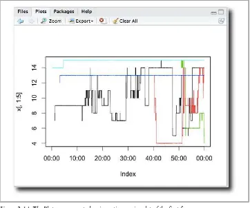
> plot(x[, 1:5], plot.type="single")
the Plots component is raised, showing the plot.
Command History
Noting that the individual paths are hard to distinguish once they’ve crossed, we want to add colors to the graphic. The col argument is used for this. Rather than retype the previous command, we can edit it. RStudio keeps a record of previous commands. The up and down arrow shortcuts can be used to scroll through our command history. For
more complicated usage, we can use the History component, which allows us to browse
the past commands and reissue them. We use the up arrow for this case, then modify the col argument to a simple value of 1:5, producing Figure 2-14.
The default plots are on the small side. Often this is all that is needed, but in this case we wish it to be bigger. The Zoom toolbar button of the Plots component’s toolbar will open the graph in a larger window.
All Finished, for Now
At this point, with the help of RStudio, we have completed the data preparation needed for subsequent analysis. We have a zoo object holding all the data (x) and a list of zoo objects (l3) storing data for individual rats. In the process of this 30-minute analysis,
we took advantage of all of RStudio’s key components: the Files browser, tab
com-pletion, the text editor, the Help browser, the rectangular data viewer, the Console, the Source code editor, the Packages browser, and the Plots viewer.
CHAPTER 3
The Console and Related Components
Interactive use of R is achieved through the command-line interface (CLI) provided by the Console component—this is where users issue commands for R to evaluate. RStudio provides a console that behaves very much like most other consoles R users have seen, such as the one provided by the RGui for Windows. This chapter describes command-line usage in RStudio, along with some of the components providing direct support for interactive usage.
Entering Commands
The simplest use of R involves typing one or more commands at the prompt (usually a
> symbol) and then pressing the enter key. Commands can be combined on one line if separated by a semicolon and can extend over multiple lines. Once entered, the com-mand is sent back to the R interpreter. If the comcom-mands are complete and there are no errors, R returns the output from the call. Usually, this output is displayed in the Console. The first command in Figure 3-1 shows how RStudio responds to the com-mand to add 2 and 2. To distinguish parts of the text, the comcom-mands appear in one color and the output in another (by default). Some calls (e.g., assignment, graphic commands, function calls returned by invisible) return no printed output. In the RStudio console, the input and output may be perused by the user and copy-and-pas-ted, but may not be directly edited.
When a command is not complete, R’s parser will recognize this and allow the user to type onto the following line. In this case, the prompt turns to the continuation prompt (typically a +). Multiline commands can be entered in this manner. The last
command in Figure 3-1 shows an example of the continuation prompt.
When a command containing an error is issued, RStudio returns the appropriate error
message generated by R (Figure 3-2). For the experienced user, these error messages
are usually very informative, but for beginning users they may be difficult to interpret.
Many commands involve assignment to a variable. R has two commonly used options for assignment: = and ← (the latter is preferred by most longtime R users). The arrow assignment operator has a keyboard shortcut Ctrl+- (Cmd+- in Mac OS X), which makes it as easy to enter as the equals sign. Using the arrow is recommended—and as a bonus, extra space is inserted around the assignment operator for clarity.
The Console panel adds very few actions. As such, there is no toolbar. The current working directory (getwd) appears in the panel’s title, along with an arrow icon to open the Files browser to display this directory’s contents. The Files browser, by design, does not track the current working directory—but the title bar does, so this arrow can be a time saver.
The width option (getOption("width")) is consulted by many of R’s functions in order to control the number of characters per line used in output. This value is conveniently updated when a user resizes the horizontal space allocated to the Console. Other options are also implemented to modify the various prompts, such as prompt and continue. There are few instances where things can get too long:
Commands with lengthy output
When the output of a command is too lengthy, it will be truncated. The option max.print will be consulted to make this determination. For server usage, one may wish to keep this small, as the data must be passed back from the server to be shown.
Figure 3-1. The first command shows printed output; the second one has a continuation prompt appear, as the command is syntactically valid but not complete during evaluation
Commands with lengthy run times
Sometimes a command will take a long time to execute. This may be by design, but it also can be the result of an erroneous request. In the first case, one can inform the user of the state (e.g., ?txtProgressBar). In the latter case, a user may wish to interrupt the evaluation. This is done using the Escape key or by clicking on the Stop icon that appears during a command’s execution in the Console pane’s title bar (Figure 3-3).
Figure 3-3. An icon to interrupt a command’s evaluation appears during long-running commands
Automatic Insertion of Matching Pairs
In R, many characters come in pairs: parentheses, brackets, braces, and quotes ((, [, [[, ", and '). Failing to have a matching pair will often result in a parsing error or an incomplete command, both annoyances. RStudio tries to circumvent this by automat-ically creating matching pairs when the first one is entered. That is, typing a left pa-renthesis adds a matching right one. Also, deleting one will can cause the other to be deleted if no text is entered in between.
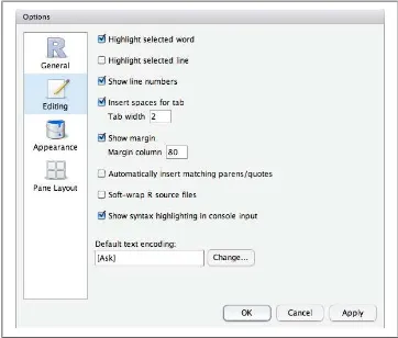
While very useful, this feature can be hard to get accustomed to, so it can be turned off. RStudio’s Options dialog (Preferences in Mac OS X) provides a toggle button (Figure 3-4). Even if this feature is turned off, RStudio still provides assistance with matching pairs by highlighting the opening parenthesis, bracket, or brace when the cursor is positioned at the closing one.
R Script Files
The console is excellent for quick interactive commands but not as convenient for longer, multiline commands. For such tasks, being able to type the commands into a file to be executed as a block proves very useful. Not only is it easier to see the underlying logic of the commands and to find any errors, this style also allows one to easily archive commands for later reference. The RStudio Source editor (described more fully in
“Source Code Editor” on page 63) can be used for writing scripts and executing blocks of code from them.
A new R script file can be opened in the code editor using the leftmost toolbar button on the application toolbar or from the File > New > R Script menu item. Into this file a series of commands may be typed. There are different actions available that execute these commands in part or in total:
Run line or selection
Run the current line or selection. Commands that are run are added to the history
stack (“Command History” on page 36).
Run all lines
Run all the lines in the buffer.
Run from beginning to line or run from line to end
Run lines above or below the current line.
Run function
Have RStudio look for the function enclosing the cursor and run that.
Rerun previous region
This allows one to edit a region and rerun its contents without needing to reselect it.
Source (or Source with echo)
Call source on the file ("source with echo” will echo back the commands). Sourced commands do not add to the history stack.
These actions are invoked via the menu bar, keyboard shortcut, or toolbar button. All
appear under the Edit > Run Code menu item and have their corresponding keyboard
shortcut shown (Table 3-2). The toolbar buttons for the editor allow one to run the
line or selection quickly, rerun the previous region, or source the buffer into R.
Command-Line Conveniences
Working with a command line has a long history. Despite the popularity of GUIs, command lines still have many aficionados, as they are more expressive—and, once some conveniences are learned—usually much faster to use. For reproducible research they are great, as they can record the exact commands used. There are drawbacks, though. Typing can be a chore, proper command syntax is essential, and the user needs to have intimate knowledge of the function and its arguments. All of these can be huge obstacles to newcomers to R. Over time, these drawbacks of command-line usage have been lessened through techniques such as tab completion, keyboard shortcuts, and history stacks.
We discuss RStudio’s implementation of these next. Becoming well-versed in these features can help you turn the command line from a distant stranger into a welcome friend.
Tab Completion
Working at the command line requires users to remember function names and the names of their arguments. To save keystrokes, many R users rely on tab completion to complete partially typed commands. The basic idea of tab completion is that when the user has a partially completed command and the Tab key is pressed, the command will be completed if there is only one candidate for completion. If there is more than one, a menu of candidates is given. The implementation of this feature varies across the different R interfaces, although most implement it—none, perhaps, as intuitively as RStudio. Here the menu provided for candidate selection is a context-sensitive com-pletion dialog raised (when needed) by pressing the Tab key and dismissed by making a selection or by pressing either the Backspace or Escape key.
The completion dialog (see Figure 3-5) has a left pane with options that can be scrolled through, and usually a right pane providing details on the selection (if available). This short description is great for jogging memories as to what the value does. The corre-sponding help page that contains this information can be opened by pressing the F1 key. A candidate value for completion may be selected with a mouse, but it is typically more convenient to use the keyboard. Press the up or down arrow to scroll through the list and use the Enter key (or Tab key again) to select the currently highlighted value for insertion. Typing a new character will narrow the list of candidates.
The completion window depends on the context of the cursor when the Tab key is pressed. Here are some scenarios:
Completion of object and function names
When an object or function name is partially typed, the completion candidates will be objects on the user’s search path whose case-sensitive name begins with the value. Objects may be in the global workspace of the user or available objects from the loaded packages (functions, variables, and data sets). In the latter case, the package name appears next to the value and, when possible, a summary of the object from its help page (Figure 3-5).
Figure 3-5. Completion for an object in the workspace shows the full name, its package (when applicable), and a short description if available
Listing of function arguments
Figure 3-6. The completion window for function arguments shows information from the help page
Completion within a function’s argument list
Within a populated argument list, the completion code provides arguments and objects, as both may be desired (Figure 3-7). R can use named arguments or posi-tional arguments where only the object is specified.
Figure 3-7. Completion with a function from a partial description shows that candidates include arguments and objects
Completion within strings
Within quotes, the completion code will offer a list of files and subdirectories to choose from (Figure 3-8). By default, this will list files and directories in the working directory, but if any part of a path is given (absolute or using the “tilde” expansion) then files and directories relative to that are presented.
The selection of completion candidates is eventually delegated to a framework provided by R’s utils package and documented under rcompgen. That help page has much more detail on how the completion candidates are figured out. For example, completion can be done after the extractors $ (for lists and environments) and @ (for S4 objects). In this case, the completion window has no details pane. Additionally, completion can be carried out inside namespaces, even when not ex-ported.
There are a few limitations of the completion mechanism. Completion of function arguments can be difficult for generic functions, as the ar-gument list may depend on the specified arar-guments and these are not evaluated; and the token for completion is found by considering the current line, so it doesn’t work well with multiline commands.
Keyboard Shortcuts
Keyboard shortcuts allow the user to quickly invoke common actions by pressing the appropriate keyboard combination. For example, many people have their fingers trained for the copy and paste keyboard shortcuts, as using them can be more conven-ient than using a mouse to initiate these actions. RStudio has numerous keyboard shortcuts. In keeping with standard GUI design, many of these appear alongside the menu item associated with the action. Here, we discuss those shortcuts that are im-plemented for the console and its integration with the source-code editor.
Keyboard shortcuts are usually operating-system dependent, and RStudio’s are no ex-ception (though, they are not locale specific). Additionally, keybindings may also be editor-dependent. In particular, the well-established vi and emacs keybindings are hardwired into many users’ fingers. The RStudio keybindings are a mix of OS-consis-tent bindings (e.g., copy and paste in Windows is Ctrl+C and Ctrl+V, and in Mac OS X, Cmd+C and Cmd+V) and Emacs-specific (e.g., Ctrl+K will kill all the text to the right of the cursor [including the end-of-line character] and Ctrl+Y will yank it back [paste it in]). Although vi users may feel left out, adding in the Emacs bindings surely
makes many longtime R users happy—it is hard to retrain one’s fingers! Similar short-cuts have been present for a long time in R’s console through the readline library. In Table 1-2, we listed shortcuts for navigation between components. Here in Ta-ble 3-1, we describe shortcuts for working at the console, and in Table 3-2 list the available shortcuts for sending commands from the source-code editor to the console. General editing shortcuts for the console and source editor are listed later in Table 5-1.
In RStudio, keybindings are currently not customizable. Keeping con-sistency across platforms, the web interface, and the Qt desktop is dif-ficult. Keyboard shortcuts do get updated on occasion. The current list is found under the menu item Help > Keyboard Shortcuts.
Table 3-1. Console-specific keyboard shortcuts
Description Windows and Linux Mac
Move cursor to console Ctrl+2 Ctrl+2
Clear console Ctrl+L Command+L
Move cursor to beginning of line Home Command+Left
Move cursor to end of line End Command+Right
Navigate command history Up/Down Up/Down
Pop-up command history Ctrl+Up Command+Up
Interrupt currently executing command Esc Esc
Change working directory Ctrl+Shift+D Ctrl+Shift+D
Table 3-2. Keyboard shortcuts for running commands in the Source editor
Description Windows and Linux Mac
Run current line/selection Ctrl+Enter Command+Enter
Run current document Ctrl+Shift+Enter Command+Shift+Enter
Run from document beginning to current line Ctrl+Shift+B Command+Shift+B
Run from current line to document end Ctrl+Shift+E Command+Shift+E
Run the current function definition Ctrl+Shift+F Command+Shift+F
Rerun previous region Ctrl+Shift+P Command+Shift+P
Source a file Ctrl+Shift+O Command+Shift+O
Source the current document Ctrl+Shift+S Command+Shift+S
Command History
Interactive usage often involves repeating a past command or parts of a command. Perhaps one wishes to change an argument’s value, or perhaps there was a minor error. Retyping an entire command to make a minor change is tedious at best. A common instinct is to insert the cursor at the error and edit the previously issued command, but this is not supported by the RStudio console. One might then be tempted to copy and paste the command to the prompt and proceed to edit.
The history mechanism speeds up this process. RStudio keeps a stack of past commands and allows one to scroll through them easily. This can be done using the up and down arrow keys. As the arrows are pressed, the previous commands are copied to the prompt, allowing them to be edited. The list of commands can be scrolled through quickly.
To see more than one previous command at a time, the Ctrl+Up keyboard shortcut can be typed, and a history window, similar to that for tab completion, will pop up (Figure 3-9).
Searching the history stack
Searching (as opposed to scrolling) through the past history (Ctrl+R on many R con-soles) is better for lengthy sessions. RStudio implements searching its own way. Calling Ctrl+Up when there is text already typed at the prompt will narrow the list shown in the history pop up to just commands beginning with that text. One can use the arrow keys or mouse to select a value. Alternatively, one can continue typing, which causes the pop up to close and reopen with a narrowed list.
History Browser
In addition to the command-line interaction with a user’s history, RStudio also provides a History browser (Figure 3-10), allowing the user to scroll through past commands or use a search box. The past commands are organized in time order, with timestamps added for extended sessions. By default, this component resides in a tab in the notebook on the upper right, and may be raised by clicking on the tab or using the shortcut Ctrl +4.
The basic usage involves double-clicking a line, which sends it to the console to be edited or reissued (the focus shifts to the console, so just pressing the Enter key will re-execute the command). Other uses involve first marking a selection. A single click selects the line, and this selection can be extended by holding the Shift key and using the up and down arrows. Other selection modifications are also possible. The compo-nent’s toolbar has three buttons: one sends the selection to the console, one appends the selection to a file in the source-code editor, and one removes the selection from the history list (the page icon with the red “x”). If a multiline selection is sent to the console, no continuation prompt is inserted, allowing one to edit any of the lines.
The toolbar also has icons to save the history to a file, read the history in from a file, and clear the history in its entirety.
Figure 3-10. The history component shows the session history, which allows commands to be recycled
The General panel of the options dialog has a couple of entries related to the history-recording mechanism: one to modify how the history is saved and one to toggle the option to remove duplicate commands.
Workspace Browser
When an R user assigns a value to a variable, the assignment is held in an
environ-ment, R’s way of organizing its objects. The R user has provided them with a global
workspace (.GlobalEnv), which is a top-level environment where names are bound during interactive use (Figure 3-11). This workspace is typically persistent—that is, a user is prompted to save it when quitting an R session, and it is loaded on startup or
when a new project is selected (see “Which Workspace?” on page 7). Over time, there
can be many variables, and remembering what they are can become nearly impossible. R has some functions to list the values in an environment (primarily ls), but RStudio makes this much easier through its Workspace browser.
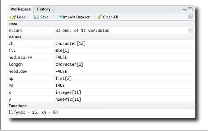
The Workspace browser appears by default in the notebook in the upper-right pane of the GUI. The browser lists the objects in the global workspace, organized by type of value: Data, Values, Functions.
Figure 3-11. The workspace browser component summarizes objects in the global workspace; objects can be viewed or edited
Editing and Viewing Objects
Clicking on a value will initiate an action to edit or view the object. Currently, rectan-gular objects, such as data frames and matrices, are not editable. For these, RStudio provides an implementation for View (really dataentry).
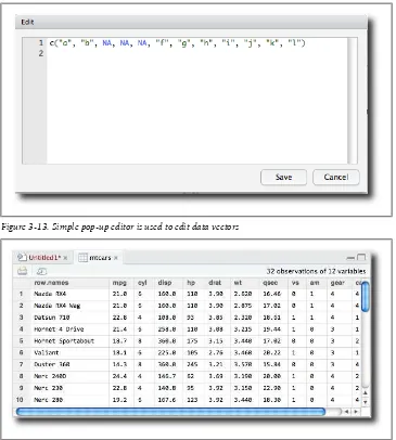
For other objects, how the value gets edited depends on the type of object and its length. For some atomic objects with length 1, the editing occurs within the Workspace browser (Figure 3-12). Clicking on the object highlights its value, which can then be edited using the browser as a property editor. The input expression is not evaluated and need not be of the same class.
Figure 3-12. Atomic objects of length 1 are edited inline
More typically, clicking on an object invokes an editor in a pop-up window. In
Fig-ure 3-13, we see the editor appearing after clicking on the ch variable, a character vector of length 12.
One can edit and save, or simply cancel. Similarly, one can edit functions through the same editor.
Editing an object involves first deparsing the object into a file and then calling the editor on that file. When editing is finished, the text is parsed and, if there is no error, this value is assigned (see ?edit for details). Editing of some objects—for instance, S4 objects —is not possible. Editing of functions preserves the function environment.
For data frames and matrices, there is a data viewer. Clicking on such an object will open a view of the data in the code-editor notebook similar to Figure 3-14. At the time of this writing, the view is limited to 100 columns and 1,000 lines. This view is a snap-shot and is not updated if the underlying object changes. However, reclicking the object in the Workspace browser will refresh the view.
Figure 3-14. The data-frame viewer provided by RStudio is rendered in the Source-editor notebook
The Workspace browser has a few other features available through its toolbar for ma-nipulating the workspace:
• Previously saved workspaces (or the default one) can be loaded through a dialog invoked by the Load toolbar button.
• The current workspace can be saved either as the default workspace (.RData file) or to an alternate file.
• The entire workspace can be cleared through the Clear All toolbar button. To delete single items, one can use the rm function through the console.
Just around the corner…
The Workspace browser is likely to see many new features as RStudio matures. For example, a data editor for matrices and data frames, a workspace filter, and a way to delete individual items could all be added.
Importing Data Sets
Importing data into an R session can be done in numerous ways, as there are many
different data formats. The R Data Import/Export manual provides details for common
cases. For properly formatted text files, RStudio provides the Import Dataset toolbar button to open a dialog to initiate the process. You select where the file resides (locally, or as a web resource), then a dialog opens to select the file. Once a file is specified (and possibly downloaded/uploaded), a dialog appears that allows you to customize how the data will be imported. Figure 3-15 shows the defaults for reading in the mtcars data when first written out as a csv file.
Figure 3-15. Dialog for importing a data set from a formatted text file
The dialog has the more commonly used arguments for a call to read.table, but it is missing a few, such as comment.char.
For server usage, one can upload arbitrary files into the working direc-tory through the Files browser (see “The File Browser” on page 71).
The Help Page Viewer
As mentioned, R is enhanced by external code organized into packages. Packages are a structured means for the functions and objects that extend R. Part of this organization extends to documentation. R has a few ways of documenting itself in a package. For packages on CRAN, compliance is checked automatically. Each exported function should be documented in a help page. This page typically contains a description of the function, a description of its arguments, additional information potentially of use to the user, and, optionally, some example code. Multiple functions may share the same documentation file. In addition to examples for a function, a package may contain demos to illustrate key functionality and vignettes (longer documents describing the package and what it provides).
R has its own format, Rd format, for marking up its help pages. This format is well
described in Writing R Extensions, one of the manuals that accompanies R. As the Rd format is structured, functions (in the tools package) have been written to convert the text to HTML format. R comes with a local web server to display these pages. RStudio
can show them as well, and does so in its Help browser. By default, this component
(Figure 3-16) appears as a page in the notebook in the lower-right corner.
Help pages are invoked by the help function, although the easy-to-type shortcut ? is typically used. For example, typing ?mean will open the help page for the mean function from the base package (Figure 3-16).
An advantage of HTML rendering of help pages is that the provided links are active. For example, in the mean help page, the help page author provides links (Figure 3-17) to weighted.mean (for computing a mean with weights), mean.POSIXct (an S3 method for computing the mean of time data), and colMeans.
Figure 3-17. Help pages have active links
The add-on helpr package for R enhances the appearance of the help pages by applying attractive CSS styling, adding a comment feature, and providing the ability to execute the examples directly from the Help browser.
The ? shortcut is the most basic functionality for help. In the Packages component, the installed packages appear as a link. Clicking a package’s link opens a description page for the package. This is much more useful than the output of help(package="…"), which creates a text only display in the source-code editor. This description page gives links to the documented functions, and in addition (if applicable) provides access to the DESCRIPTION file, the NEWS file, a list of demos, and any package vignettes.
The ?? shortcut allows quicker access to R’s help.search function. This allows for searching the help system’s documentation for a match to the specific pattern, searching within the alias, title, and concept entries. (The help.search function allows a more