Facultad de Ciencias Económicas y Empresariales Universidad de Navarra
Working Paper nº 14/03
A Structural Estimation and Interpretation of the
New Keynesian Macro Model
Seonghoon Cho
Economics Department, Columbia University
Antonio Moreno
A Structural Estimation and Interpretation of the New Keynesian Macro Model Seonghoon Cho and Antonio Moreno
Working Paper No.14/03 November 2003
JEL Codes: C32, E32, E52.
ABSTRACT
We formulate and solve a Rational Expectations New Keynesian macro model that implies non-linear cross-equation restrictions on the dynamics of inflation, the output gap and the Federal funds rate. Our maximum likelihood estimation procedure fully imposes these restrictions and yields asymptotic and small sample distributions of the structural parameters. We show how the structural parameters shape the responses of the macro variables to the structural shocks. While the point estimates imply that the Fed has been stabilizing inflation fluctuations since 1980, our econometric analysis suggests considerable uncertainty regarding the stance of the Fed against inflation. Seonghoon Cho
Columbia University Economics Department 10027 New York, NY [email protected] Antonio Moreno
ACKNOWLEDGEMENTS
1
Introduction
One of the central issues in macroeconomic analysis is the impact of structural shocks on the dynamics of inflation, the output gap and interest rates. Much of the empirical analysis employs large vector autoregressive (VAR) systems which often have a difficult economic interpretation. In this paper we examine the interaction of the exogenous structural shocks with the behavior of both the monetary authority and private agents in the context of a New Keynesian macroeconomic model. We estimate the complete structural model and analyze the small sample properties of its structural parameters. We then show how the structural parameters govern the dynamic responses to structural shocks.
Our structural model comprises an aggregate supply (AS) equation based on a con-tracting specification, an IS or demand equation based on representative agent utility maximization with habit persistence, and a forward looking monetary policy rule. The Rational Expectations solution of the model implies a set of identifying assumptions which translate into cross-equation restrictions on the time series dynamics of the macro variables. This allows us to recover the effects of structural shocks and interpret the dynamics of the macro variables in response to those shocks.
Our approach makes three main contributions to the analysis of the effects of struc-tural shocks on macro variables. First, we estimate the complete strucstruc-tural model jointly, whereas many of the previous studies focused on equation by equation estimation. The estimation of the full system has the advantage of allowing for the interaction among the different economic agents: Consumers, firms and the Central Bank.
Second, we establish a tight link between structural equation parameters and the responses of the macro variables to economic shocks. This is possible because of the time series restrictions implied by the theoretical model. Our analysis can then address questions such as: “By how much does the output gap fall after a supply shock, when the Central Bank pursues a more stabilizing policy on inflation?”, “What is the relation between the Phillips curve parameter and the price puzzle?”, “Does a higher intertem-poral elasticity of substitution imply a bigger impact of the monetary policy shock on the real economy?”, or “What is the contribution of the systematic part of the Central Bank reaction function to the propagation of monetary policy shocks?”
solutions, we propose an alternative criterion that selects a solution which is bubble-free and consistent with expectations of the structural model.
We estimate the model by full information maximum likelihood (FIML).1 The
sensi-tivity analysis reveals that the more aggressively the Federal Reserve reacts to expected inflation and the output gap, the smaller impact the monetary policy shock has on the output gap and inflation. In addition, when the Federal Reserve greatly smooths inter-est rates, the effect of the monetary policy shock is amplified. We find that the more private agents smooth consumption across periods, the less effective the monetary pol-icy shock is on real activity. The effect of the monetary surprise on inflation is very modest: The small estimate of the Phillips Curve parameter in the AS equation, which governs the direction and the size of the inflation response to the monetary policy shock in our baseline model, implies a high degree of inflation rigidity. The AS shock in turn moves the output gap and inflation in opposite directions. We show that the output gap decrease is exacerbated by a more than one to one reaction of the Central Bank to expected inflation. However, while our point estimate of the Fed’s response to expected inflation during the 80’s and 90’s is above unity, it is not significantly so. Finally, a more stabilizing response of the Fed to deviations of the macro variables from their targets unambiguously dampens the impact of the IS shock on inflation and the output gap.
In order to conduct more precise inference about the implications of the structural model, we perform a bootstrap exercise which yields the empirical probability distribution of the structural parameters. Two main empirical facts emerge from this small sample analysis. First, it confirms that the estimate of the Fed’s reaction to expected inflation is not significantly above one and reveals that it is upwardly biased. Second, the empirical distributions of both the Phillips curve parameter and the coefficient relating the output gap and the real interest rate in the IS equation are very different from their asymptotic distributions. This finding indicates that frequently used measures of output gap, such as linearly or quadratically detrended output, contain considerable measurement error.
Even though the original model is strongly rejected using the likelihood ratio (LR) test, our analysis shows that when the error terms of the model are allowed to be serially correlated, the model is only marginally rejected at the 5% level using the small sample distribution of the LR test statistic.
1In order to avoid the potential problem of parameter instability, we select a sample period,
The paper is organized as follows. Section 2 discusses the related literature. Section 3 lays out the complete but parsimonious model of the macroeconomy. In section 4 we discuss the Rational Expectations solution of the model and describe our new methodol-ogy to handle the potential multiplicity of solutions. Section 5 describes our estimation procedure. Section 6 discusses the data and the selection of the sample period based on the sup-Wald break date test statistic. In Section 7 we present our results. First we show the estimates of the structural model and implied dynamics. Then we perform a small sample study which allows us to develop our sensitivity analysis. Finally we carry out model diagnostics using the asymptotic and small sample LR tests. Section 8 concludes.
2
Related Literature
A popular strategy to identify structural policy shocks is to estimate empirical VAR systems. VAR studies recover the implied dynamics of the macro variables following structural shocks by placing a sufficient number of exclusion restrictions. Blanchard and Quah (1989), Leeper, Sims, and Zha (1996) or Christiano, Eichenbaum, and Evans (1999) are examples of this approach. In our study, by imposing a structural model, we do not need to impose these zero restrictions and all the variables are contemporaneously related. Even though the fit to the data cannot be as accurate as in large VAR systems, our Rational Expectations model solution provides a natural structural interpretation of the macro dynamics.
Our structural model is a linearized Rational Expectations model consisting of AS, IS and monetary policy rule equations with endogenous persistence. The AS equation is a modified version of the real wage contracting equation in Fuhrer and Moore (1995). We derive the IS equation through representative agent optimization with external habit persistence, as in Fuhrer (2000). The monetary policy rule in our model is the forward looking Taylor rule proposed by Clarida, Gal´ı, and Gertler (2000). Our model, though parsimonious, is rich enough to capture the macro dynamics implied by recently devel-oped New Keynesian models so that the dynamic paths of inflation, the output gap and the interest rate can be clearly explained in terms of the structural parameters.
the structural parameters obtained through estimation provide a more reliable analysis of the model dynamics. Second, our FIML estimation is more efficient than instrumental variables techniques such as Generalized Method of Moments (GMM). The implications of our policy rule estimates differ from those of Clarida, Gal´ı, and Gertler (2000), who estimate the policy reaction function by GMM. Third, we estimate the complete macro model jointly, whereas McCallum and Nelson (1998), Gal´ı and Gertler (1999) and Rude-busch (2002) estimate the structural equations separately. The joint estimation has the advantage that it accounts for the simultaneous effect of all the structural shocks on each of the variables in estimation.2
A closely related paper is Ireland (2001), who estimates a New Keynesian model based on explicit microfoundations by maximum likelihood. His analysis contains, how-ever, two main differences with respect to our study. First, the equations of our model display endogenous persistence, whereas in his case the persistence is imposed exoge-nously. Second, and more importantly, while he focuses on studying the instability of the model parameters, our main interest is to interpret the macroeconomic dynamics following the structural shocks in terms of the structural parameters of the model. In order to draw a sharper inference, we perform a small sample study of the structural parameters which accounts for parameter uncertainty.
Finally, we construct an alternative procedure to solve Rational Expectations systems that selects the economically relevant solution in the case of multiplicity of stationary solutions. It differs from the minimal state variable criterion developed by McCallum (1983) in that it yields a bubble-free solution by solving the model forward recursively.
3
The Model
We characterize the set of macroeconomic relations through the following system of 3 equations: The AS or Supply equation, the IS or Demand equation and the forward
2Rotemberg and Woodford (1998), Amato and Laubach (1999), Christiano, Eichenbaum, and Evans
looking monetary policy equation. Each of them exhibits endogenous persistence, which allows for more realistic dynamics in the macroeconomy, and a forward looking part. We assume that there is no informational difference between the private sector (firms and households) and the Central Bank.
3.1
AS Equation
The AS equation or “New Phillips Curve” describes the short run inflation dynamics as a result of the wage setting process between firms and workers. We generalize the AS equation rationalized by Fuhrer and Moore (1995), who present a model of overlapping wage contracts in which agents care about relative real wages:
πt=αAS +δEtπt+1+ (1−δ)πt−1 +λ(yt+yt−1) +ǫASt (1) αAS is a constant. πt and yt stand for inflation and the output gap betweent−1 and t,
respectively, and ǫASt is the aggregate supply structural shock, assumed to be
indepen-dently and identically distributed with homoskedastic variance σ2
AS. Et is the Rational
Expectations operator conditional on the information set at time t, which comprises πt,
yt, rt (the nominal interest rate at time t) and all the lags of these variables. As can be
seen in equation (1) inflation depends not only on expected future inflation but also on lagged inflation with weights δ and 1−δ, respectively.3 ǫ
ASt can be interpreted as a cost
push shock that deviates real wages from their equilibrium value or simply as a pricing error. One advantage of this specification is that it captures the inflation persistence that is present in the data. Gal´ı and Gertler (1999) also impart persistence to the inflation rate by letting a fraction of firms use a backward looking rule of thumb to set prices.
3.2
IS Equation
The IS equation describes the demand side of the economy. It is derived by a represen-tative agent model in Fuhrer (2000), with the utility function given by
U(Ct) =
(Ct
Ht)
1−σ −1
1−σ (2)
3Forα
whereCtis the consumption level,Htis the external level of habit and σis the inverse of
the elasticity of substitution. The habit level is external in the sense that the consumer does not consider it as an argument to maximize his utility function. We assume that
Ht=Cth−1 ex post, whereh (>0) measures how strong the habit level is. It is the habit
specification that will introduce persistence in the IS equation. The budget constraint that the agent faces is
Ct+Bt≤
Pt−1
Pt
Bt−1Rt+Wt (3)
This constraint implies that agents’ consumption at time t,Ct, plus the value of his asset
holdings, Bt, cannot exceed his endowment each period, which comes from labor income,
Wt, and the real value of the asset holdings that he had at the beginning of the period, Pt−1
Pt Bt−1, multiplied by the nominal gross return on those assets, Rt.
The agent is infinitely lived and maximizes his lifetime stream of utility, subject to the dynamic budget constraint in (3). The Euler equation is given by
1 = Et[ψ
whereψ is the time discount factor andPt is the price level at timet. By assuming joint
lognormality of consumption and inflation, the following expression can be derived:
ct=αC +µEtct+1+ (1−µ)ct−1−φ(rt−Etπt+1) (5)
in equation (5), the monetary transmission mechanism is a function of the inverse of the elasticity of substitution of consumption across periods,σ, and the habit persistence parameter, h.
From the market clearing condition,Y∗
t =Ct+Gt, where Y ∗
t is the aggregate supply
andGtdenotes the remaining demand components: investment, government expenditures
and net exports. Taking logs, ct = y
t and yt is the output gap. Then, equation (5) can be rewritten as:
wheregt =−(zt+ytT) +µEt(zt+1+yt+1T ) + (1−µ)(zt−1+yTt−1). Note thatytrises withGt.
Finally, define αg =Egt, whereE is the unconditional expectation operator, in order to
rewrite the IS equation as
yt=αIS +µEtyt+1+ (1−µ)yt−1−φ(rt−Etπt+1) +ǫIS,t (7)
where αIS =αC+αg and ǫISt =gt−αg.
4 We will interpret ǫ
IS,t as an exogenous shock
to aggregate demand throughout the paper.5 Since we do not modelG
texplicitly,ǫIS,t is
assumed to be independent and identically distributed with homoskedastic variance σ2IS.
3.3
Monetary Policy Equation
The instrument of the monetary authority, the Federal funds rate,6 is set according to
the following reaction function proposed by Clarida, Gal´ı, and Gertler (2000):
rt = ρrt−1+ (1−ρ)r ∗
t +ǫM Pt (8) r∗
t = ¯r ∗
+β(Etπt+1−π¯) +γyt (9)
¯
π is the long run equilibrium level of inflation and ¯r∗
is the desired nominal interest rate. There are two parts to the equation. The lagged interest rate captures the well known tendency of the Federal Reserve towards smoothing interest rates, whereas r∗
t,
represents the “Taylor rule” whereby the monetary authority reacts to deviations of expected inflation from the long run equilibrium level of inflation and to the current output gap. Hence, the monetary policy equation becomes:
rt =αM P +ρrt−1+ (1−ρ) [βEtπt+1+γyt] +ǫM Pt (10) 4Equation (7) can also be expressed asy
t=µEtyt+1+ (1−µ)yt−1−φ(rt−Etπt+1−rr¯) +ǫISt, where
¯
rr=αI S
φ .rr¯ represents the long run equilibrium real rate of interest.
5 Woodford (2001) points out thatǫ
ISt cannot be interpreted in general as a demand shock, since it
includes shocks to the trend component of output which could be driven, for instance, by technological innovations. However, under linear output detrending, the innovations to the output trend vanish from
ǫISt, so that ǫISt could be interpreted as a demand shock. Under quadratic output detrending, even
though a deterministic trend component remains inǫISt, its size is negligible so that our empirical results
are virtually unaffected. The interpretation of ǫISt as a demand shock under other filters, such as the
Congressional Budget Office measure of potential output, is clearly more problematic.
αM P = (1−ρ)(¯r∗ −βπ¯) and ǫM Pt is the monetary policy shock, that we are trying to
identify. It is assumed to be independently and identically distributed with homoskedastic variance σM P2 .
4
Rational Expectations Solution
4.1
Model Solution and Implications
In this section we derive the Rational Expectations solution of the model and analyze its properties. Our macroeconomic system of equations (1), (7) and (10) can be expressed in matrix form as follows:
ters, andαis a vector of constants. ǫtis the vector of structural errors,Dis the diagonal
variance matrix and 0 denotes a 3×1 vector of zeros.7 By assuming Rational
Expec-tations and no asymmetric information between the economic agents and the monetary policy authority, we can write:
Xt+1 =EtXt+1+vt+1 (12)
where vt+1 is the vector of Rational Expectations errors. Following a standard
Undeter-mined Coefficients approach, a bubble-free solution to the system in (11) can be written as the following reduced form:
Xt+1 =c+ ΩXt+ Γǫt+1 (13)
wherecis a 3×1 vector of constants and Ω and Γ are 3×3 matrices. To see this, substitute equation (13) into equation (11) and rearrange by applying Rational Expectations. Then:
(B11−A11Ω)Xt =α+A11c+B12Xt−1+ǫt (14)
Linear independence among the 3 structural equations implies nonsingularity of (B11−
A11Ω). Thus we assume that (B11−A11Ω) is nonsingular in what follows. Then,
pre-multiply by (B11− A11Ω)−1 on both sides in equation (14) and match the coefficient
matrices of Xt−1 and ǫt, to obtain:
Ω = (B11−A11Ω) −1
B12 (15)
Γ = (B11−A11Ω)−1 (16)
c = (B11−A11Ω−A11) −1
α (17)
Therefore, equation (13) with Ω, Γ and c satisfying equations (15), (16) and (17) is a solution to equation (11). Once we solve for Ω as a function of A11, B11 and B12, Γ
and ccan be easily calculated. A detailed solution method will be given in the following subsection. Notice that the implied reduced form of our structural model is simply a VAR of order 1 with highly nonlinear parameter restrictions. Furthermore, there is a simple linear relation between Ω and Γ through B12, which captures the dependence of
the system on the lagged predetermined variables.
Ω = ΓB12 (18)
Note also that there is a linear relation between the structural errors,ǫtand the reduced
form errors (Rational Expectations errors), vt, through Γ,
vt= Γǫt (19)
A pure forward looking system implies B12 = 0 in our system, and the implied reduced
form is simply Xt+1 = c+ Γǫt+1 where Ω = 0 and Γ = B11−1. Since in this case there
statistical selection methods such as the Schwarz and Akaike criteria often lead monetary policy analysis to choose higher order VARs.8 Although such models fit the data better, as
Clarida, Gal´ı, and Gertler (1999) point out, it is a daunting task to justify macroeconomic models which include more than one lag. The model we are working with in this paper lies between these two approaches: The three equations we consider have a theoretical justification and they also feature persistence of the variables.
4.2
Characterization of the Rational Expectations Solution
Rewrite equation (15) as:
A11Ω2−B11Ω +B12 = 0 (20)
Once Ω is solved for, Γ and c, the remaining unknown matrices in equation (13), follow directly from equations (16) and (17). For Ω satisfying (20) to be admissible as a solution, it must be real-valued and exhibit stationary dynamics. Because Ω is a nonlinear function of the structural parameters in B11, A11 and B12, there could potentially be multiple
stationary solutions or no stationary solutions at all. Additionally, the existence of a complex valued solution cannot be ruled out. The singularity of the matrixA11is another
difficulty in solving (20).
We employ two different methods to solve equation (20). First, we utilize the general-ized Schur (QZ) Decomposition in solving Rational Expectations models. We will follow Uhlig (1997), as he proposes an approach which is closely related to the QZ method.9
The QZ method is particularly useful when the matrix A11 is singular, which is the
case in our model, and it allows us to determine whether there exists a stationary,
real-valued bubble-free solution. Specifically, define the 2n ×2n matrices A =
"
A11 0
0 I
#
and B =
"
B11 −B12
I 0
#
where n is the number of endogenous variables. The set of all matrices of the form B −λA with λ ∈ C is said to be a matrix pencil and λ is called a generalized eigenvalue of the pencil. Define Λ be the diagonal matrix whose diagonal elements are the eigenvalues and S be the eigenmatrix with each column corresponding
8Rudebusch and Svensson (1999), for instance, use a backward looking model.
9Even though Uhlig’s formula only requires to compute the generalized eigenvalues and eigenvectors,
to its eigenvalue such that BS =ASΛ. Then: Ω =S21Λ11S
−1
21 (21)
satisfies equation (20) where Sij and Λij are the n×n ij-th submatrices of S and Λ,
respectively. We can characterize the stationarity, uniqueness and real-valuedness as follows: If all the eigenvalues of Λ11 are less than unity in absolute value, then Ω is
stationary. If the number of stable generalized eigenvalues is the same as that of the predetermined variables (3 in our model, the lagged endogenous variables), then there exists a unique solution. If there are more than 3 stable generalized eigenvalues, then we have multiple solutions. Conversely, if there are less than 3 stable eigenvalues, there is no stable solution. Finally, Ω is real-valued if (a) every eigenvalue in Λ11 is real-valued,
or (b) for every complex eigenvalue in Λ11, the complex conjugate is also an eigenvalue
in Λ11.
Unfortunately, in the case of multiple stationary solutions, there seems to be no agreement about the selection of a solution among all the candidates.10 In this case, by
solving the model forward recursively, we propose an alternative simple selection criterion that is bubble-free and real-valued by construction. The idea is to construct sequences of convergent matrices, {Ck,Ωk,Γk, k = 1,2,3, ...} such that:
¯
Xt =CkEtX¯t+k+1+ ΩkX¯t−1+ Γkǫt (22)
where ¯Xt = Xt−EXt. We characterize the solution that is fully recursive as follows.
We check first whether Ω∗
≡ lim of the solutions obtained through the QZ method. For the limit to equation (22) to be a bubble-free solution, lim
k→∞CkEt
¯
Xt+k+1 must be a zero vector. Then the solution must
be of the form:
Finally, we check whether lim
k→∞CkEt
¯
Xt+k+1 = lim k→∞CkΩ
∗k = 0 using equation (23). We
will call this the recursive method. The complete procedure is detailed in the Appendix. While the QZ method can determine whether there exists a stationary real-valued
10Blanchard and Kahn (1980) suggest the choice of the 3 smallest eigenvalues and McCallum (1999)
suggests the choice that would yield Ω = 0 if it were the case that B12 = 0. Uhlig (1997) points out
solution within the class of no bubble solutions, it does not give any information about which solution should be chosen in the case of multiple solutions. In this case we select the solution from the recursive method. On the other hand, while the recursive method produces a stationary solution if it exists, one does not know whether the solution is unique or not. Hence these two methods are complementary so that they can be used jointly as a criterion to select the economically relevant solution.
5
Full Information Maximum Likelihood Estimation
We estimate the structural parameters using FIML by assuming normality of the struc-tural errors. Our FIML estimation procedure allows us to obtain the strucstruc-tural parame-ters and the VAR reduced form in one stage, affording a higher efficiency than two-stage instrumental variables techniques such as GMM. Gal´ı and Gertler (1999) and Clarida, Gal´ı, and Gertler (2000) estimate separately by GMM some of the equations of the model that we study. It seems adequate to estimate the whole model jointly, given the simul-taneity between the private sector and the Central Bank behavior, as explained by Leeper and Zha (2000).
The log likelihood function can be written as:
lnL(θ|X¯T,X¯T−1, ...,X¯1) = T
X
t=2
·
−32ln 2π− 1
2ln|Σ| − 1
2( ¯Xt−Ω ¯Xt−1) ′
Σ−1
( ¯Xt−Ω ¯Xt−1)
¸
(24) where θ = (δ, λ, µ, φ, ρ, β, γ, σAS2 , σ2IS, σM P2 ), the vector of the structural parameters and Σ = ΓDΓ′
6
Data description and sample selection
We estimate the model with U.S. quarterly data from 1980:4Q to 2000:1Q. Implicit GDP deflator data is used for inflation. The inflation rate is computed as the log difference of the GDP deflator between the end and the beginning of each quarter. The Federal funds rate is the monetary policy instrument: We use the average of the Federal funds rate over the previous quarter. Our results are by and large robust to the use of the Consumer Price Index (CPI) for inflation and the 3 Month T-Bill rate for the short term interest rate. We use three different measures for the output gap: Output detrended with the Congressional Budget Office (CBO) Measure of Potential GDP, linearly and quadratically detrended real GDP.11 The data is annualized and in percentages. Federal
funds rate data was collected from the Board of Governors of the Federal Reserve website. Real GDP and the GDP deflator were obtained from the National Income and Product Accounts (NIPA).
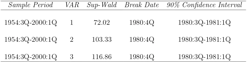
Clarida, Gal´ı, and Gertler (1999), Boivin and Watson (1999) and others have shown evidence of parameter instability across sample periods. We select our sample period based on the sup-Wald statistic for parameter instability, derived by Bai, Lumsdaine, and Stock (1998). This statistic detects the most likely date for a break in all the parameters of a reduced form VAR. We run the sup-Wald statistic for unconstrained VARs of order 1 to 3. As shown in Table 1 and in Figure 1, the beginning of the 4th quarter of 1980, one year after Paul Volcker’s beginning of his tenure as Federal Reserve chairman, is clearly identified as the most likely break date for the parameters of the reduced form relation. In all three cases, the value of the Sup-Wald statistic is significant at the 1% level12 and the the 90% confidence interval is very tight, including only three
quarters. The break date test is also robust across output gap measures. This date coincides with the biggest increase, between two quarters, in the average Federal funds rate during the whole sample: From 9.83% in the 3rd quarter of 1980 to 15.85% in the 4th. This severe contraction engineered by the Federal Reserve lies at the root of the
11The Hodrick Prescott filter, linear filter, quadratic filter and the CBO Measure of Potential GDP
have been used extensively in the literature. There seems to be no consensus about the choice of filter to generate the output gap, since all of them seem to contain some measurement error. Gal´ı and Gertler (1999) introduce a real marginal cost measure in a Calvo-type AS equation which yields better results than any of the filtered variables above. However, since our AS specification comes from a contracting model, and we estimate the complete macro model, we do not use their measure.
early 80’s disinflation.13 We start the sample right after the break date occurs.14
[Insert Table 1 Here]
[Insert Figure 1 Here]
7
Empirical Results
In this section we present our empirical findings. First, we report the structural parameter estimates and their statistical properties. Then we provide the parameters’ small sample distributions based on a bootstrap exercise. The second part of this section is devoted to the analysis of the impulse response functions of the variables to the monetary policy shock as well as the other structural shocks. In the following subsection, we present our main empirical results: We show how changes in the structural parameters around the estimated values affect the propagation mechanism of structural shocks through a sensitivity analysis. Finally, we perform specification tests of the structural model based on the asymptotic and small sample LR test statistic.
7.1
Parameter estimates
7.1.1 Structural parameters
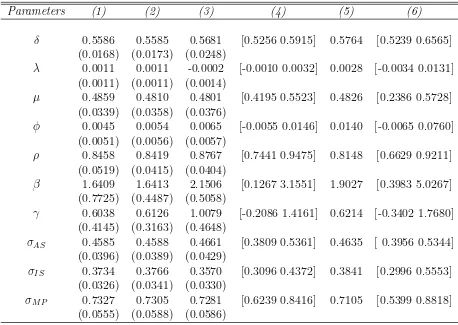
FIML estimates are shown in Table 2.15 Asymptotic standard errors are obtained as
the inverse of the Hessian Matrix. We present three sets of estimates in columns (1),(2) and (3): The first one is obtained using linearly detrended output, the second one uses quadratically detrended output and the third one uses output detrended with the CBO measure of potential output. As is clear from Table 2, the estimates are reasonably robust across output gap specifications.
[Insert Table 2 Here]
The parameter estimates are by and large consistent with previous findings in the liter-ature. In the AS equation, δ is significantly greater than 0.5, implying that agents place
13Right after Volcker’s arrival, the Federal Reserve also increased the Federal funds rate sharply, but
it was decreased shortly thereafter. Feldstein (1994) dubs this episode the unsuccessful disinflation.
14Empirical results are similar if we start the sample outside the 90% confidence interval.
15Even though we estimate the model constants, we do not report the estimates, since we are interested
a larger weight on expected inflation than on past inflation. Gal´ı and Gertler (1999) found similar estimates. The Philips Curve parameter, λ, has the right sign in two of the three specifications, but it is not statistically different from 0 in any of the three cases. Fuhrer and Moore (1995) obtained estimates of similar magnitude using the same pricing specification. In the IS equation,µis statistically indistinguishable from 0.5, im-plying that agents place similar weights on expected and past output gap. The implied habit persistence parameter, h, is around 1.07 for the three output gap specifications and statistically different from 0 at the 5% level.16 Fuhrer (2000) reports 0.80 for the
habit persistence parameter in his model. The estimates of the implied inverse of the elasticity of substitution, σ, range from 73 (when output is detrended with the CBO measure of potential output) to 110 (when output is detrended linearly).17 However it is
not significantly different from 0 in any of the three specifications. This value is consid-erably larger than the ones usually employed in calibration (see McCallum (2001)), but similar to the ones found in estimation of the linearized IS equation.18 In the monetary
policy equation, the smoothing parameter, ρ, is around 0.85, reflecting the well known persistence in the short term interest rate. β, the coefficient on expected inflation, is larger than 1, but only significantly above unity at the 5% level when the output gap is detrended with the CBO measure of potential output. γ, the coefficient on output gap, is also positive and only significantly different from 0 in the specification which uses the CBO measure of potential output. While these estimates are similar to the ones found by Clarida, Gal´ı, and Gertler (1999) for the same monetary policy rule, our standard errors are considerably larger.
7.1.2 Model solution
For the first two specifications the sets of FIML estimates imply a unique stationary solution, as we describe in the Appendix. For the remainder of our discussion we will focus on the parameter estimates obtained when output is linearly detrended since their signs are fully in agreement with the theoretical model. Additionally, the linear detrending method for output allows us to interpret ǫISt as a pure demand shock, as explained in
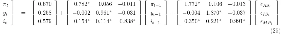
footnote 5. The estimates of the implied reduced form matrices, Ω and Γ, which drive
16Recall that µ= σ
σ(1+h)−h andφ=
1
σ(1+h)−h. Thusσ= µ
φ andh=
1−µ µ−φ.
17The statistical significance ofσin our model is difficult to interpret. Sinceσ=µ
φ,σis not normally
distributed. Additionally, since φis not statistically different from zero, inference based on first order approximation is not reliable.
the dynamics of the model, are19:
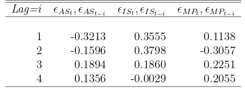
Panel A and B of Table 3 show the autocorrelation and cross correlation patterns exhib-ited by the structural errors, respectively. Panel C and D report some diagnostic tests of the residuals. The diagnostic tests give mixed results. Even though the Jarque-Bera test cannot reject the hypothesis of normality for the AS and IS residuals, the Ljung-Box Q-statistic rejects the hypothesis that their first five autocorrelations are zero.20 Under the
null of the model, there should not be significant autocorrelations or cross-correlations, but this is a very difficult test to pass given our parsimonious VAR(1) specification. The cross correlations of the error terms reveal nonzero contemporaneous correlations among the structural shocks.
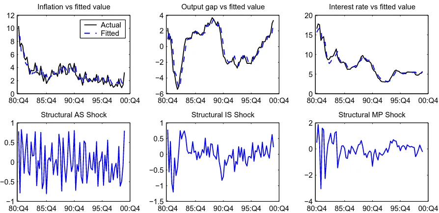
The top row of Figure 2 compares the one step ahead predicted values of the model with the actual values of inflation, the output gap and the interest rate. The predicted values generated by the model track the real values very closely. The bottom row of Figure 2 graphs the structural errors of the model. It shows that there there were not major AS shocks during the sample. The IS shocks exhibit some persistence, as reported in Panel A of Table 3. Finally, it can be seen that the monetary policy shocks were of very small magnitude after 1983. This corroborates the analysis in Taylor (1999) and Leeper and Zha (2000) showing that monetary policy shocks during the 90’s were small.
[Insert Table 3 Here]
[Insert Figure 2 Here]
7.1.3 Small Sample Distributions of the Structural Parameters
Because our sample is relatively short, inference based on asymptotic distribution may be misleading. In order to draw a more precise inference on the validity of the structural
19The stars denote the parameters that are significantly different from zero at the 5% level. The
standard errors can be calculated using delta method. Even though Ω and Γ cannot be expressed analytically in terms of structural parameters, we can derive numerical derivatives of Ω and Γ with respect to the structural parameters.
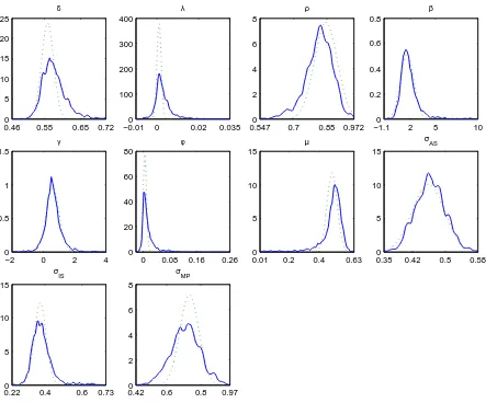
parameters, we perform a bootstrap analysis. We bootstrap 1,000 samples under the null and re-estimate the structural model to obtain an empirical probability distribution of the structural parameters. The Appendix details the bootstrap procedure. In Figure 3 we present the small sample distributions of the structural parameters. In the last two columns of Table 2 we report the small sample means of the parameters and their associated 95% confidence intervals, respectively.
[Insert Figure 3 Here]
The empirical distributions of δ and ρ are mildly positively and negatively skewed, re-spectively. This bias is related to the well known small sample downward bias of the first order autocorrelation coefficients, as reported in Bekaert, Hodrick, and Marshall (1997). The most severe small sample problem is the strong positive skewness exhibited by the empirical distribution of the Phillips curve parameter, λ, and that of the coefficient on the real interest rate in the IS equation, φ. These two parameters were not significantly different from zero in the FIML estimation. This bias present in λ and φ seems to be related to the measurement error contained in the detrended output measure. In the sensitivity analysis, we show the implications of different values of λand φ on the macro dynamics. The coefficient on expected inflation in the monetary policy rule, β, appears significantly upwardly biased, and its small sample 95% confidence interval is clearly wider than its asymptotic counterpart. In the sensitivity analysis below, we show that alternative values of β give rise to qualitatively and quantitatively different dynamics in response to the macroeconomic shocks. Finally, the averages of the empirical distribu-tions of γ and those of the three structural shocks standard deviations are very similar to the FIML parameter estimates.
7.2
Impulse Response Analysis to Structural Shocks
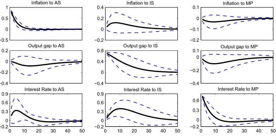
Figure 4 shows the structural impulse response functions of the variables to a one standard deviation of each shock, and the associated 95% confidence intervals.21 The units for the
responses of the variables are in percentage deviations from their steady state values. For ease of exposition, based on equation (25), we denote Ωi,j as theij-th element of Ω where
i, j = π, y, r, and Γi,j as the ij-th element of Γ where i = π, y, r and j = AS, IS, M P.
21All the impulse responses and the confidence intervals exhibit mean reversion, reflecting the
For instance, Ωy,r is the coefficient on the lagged interest rate in the IS equation and
Γπ,M P is the initial response of inflation to the monetary policy shock.
[Insert Figure 4 Here]
A contractionary monetary policy shock decreases inflation, but the impact is very small and not significantly different from zero for the whole time span. As we show in the sensitivity analysis, this is due to the sign and magnitude of the Phillips curve parameter,
λ: A positive λ ensures that prices decrease immediately after the contractionary policy shock. This precludes the appearance of the price puzzle, often obtained in empirical systems, whereby prices initially rise after an unexpected increase in the interest rate. The initial effect of the monetary policy shock on the variables can be easily identified by observing the coefficient matrix of the structural shocks, Γ. In the case of the initial effect on inflation, Γπ,M P = −0.013. Subsequently, the dynamic path of inflation is governed
by the first row of Ω.
The monetary policy shock has real effects on the economy: When the Fed surprises the economy by increasing the interest rate by 0.73%, the output gap decreases, reaching its trough of -0.1% with respect to its steady state value after 10 quarters. Γy,M P is -0.037,
so that the output gap decreases immediately after the shock. Finally, the monetary policy shock has a persistent effect on the interest rate, given the smoothing behavior of the Fed.
Since our supply curve is derived from a real wage contract and we do not model technology explicitly, the AS shock can be interpreted as a sudden increase in wages and thus the price level. The AS shock increases prices during 10 quarters. Interestingly, the Federal funds rate responds strongly (and significantly) to the AS shock (Γr,AS=0.35).
This makes the output gap decrease for a long period of time, reaching its trough,−0.8%, after 15 quarters. As we will show in the next section, this depressing effect of the AS shock is triggered by the aggressive reaction of the Fed to the inflationary pressure (β >1).
Following a positive IS or demand shock, inflation, the output gap and the interest rate exhibit a positive co-movement. This is directed by the coefficients Γπ,IS, Γy,IS and
Γr,IS, respectively, all of them larger than zero. As in the case of Γπ,M P, the sign of Γπ,IS
7.3
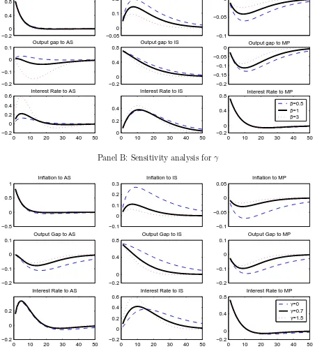
Sensitivity Analysis
Each element of Ω and Γ is a complicated function of the structural parameters. Therefore when there is a change in the systematic part of the economy, identified as a change in a structural parameter in A11, B11 or B12, all of the reduced form parameters change
simultaneously and thus affects the propagation mechanism of any structural shock. Specifically, we vary the parameters describing the systematic part of the monetary policy rule, β, γ and ρ, one at a time. We also vary some of the structural parameters in the AS and IS equations and see how the impulse responses react to these changes. This experiment amounts to an analysis of the partial derivatives of Ω, Γ, and of all the impulse response functions, with respect to the estimated structural parameter vector θ. The impact of the Lucas Critique is minimized in our setting, since the restricted reduced form varies with changes in the structural parameters.
In order to account for the uncertainty regarding the structural parameters, the range of values for this analysis is chosen from the confidence interval of the empirical distri-bution of the structural parameters, shown in column (6) of Table 2. Recall that the estimates provide a unique stationary solution. In some cases, a change in a parameter value within the confidence interval may result in a nonstationary solution or multiple solutions. Thus we choose parameter values so as to guarantee a stationary solution. In case of multiplicity of solutions, we select the one obtained through our recursive method.22 We believe that this exercise provides more information than a simple
cali-bration exercise, where lack of knowledge about the estimated value of the parameters can make the impulse responses highly misleading.
7.3.1 Changes in Systematic Monetary Policy
Clarida, Gal´ı, and Gertler (1999) and others have found that the systematic reaction to expected inflation in the monetary policy rule,β, is greater than one after 1979, implying that the Fed has been stabilizing since then. Our FIML estimate of β is also bigger than 1, but it is not significantly above unity at the 5% level. Panel A of Figure 5 shows the impulse responses when β = 0.5, 1 and 3 (which are all in the 95% confidence interval of the empirical distribution). As β increases, the Fed responds more aggressively to demand and supply shocks. A higher β also makes the private sector’s responses to the
22For instance, whenβ is less than one, there are multiple solutions, since there are 4 eigenvalues less
monetary policy shock less pronounced. This is due to the fact that the contractionary policy shock lowers expected inflation below the steady state in the future. Larger values of β partially offset the impact of the monetary policy shock, since a stronger reaction from the Fed to lower expected inflation moves the interest rate in the opposite direction to the one implied by the shock. Conversely, if the Fed is not very responsive (β = 0.5), the impact of the policy shock is magnified. These results confirm the findings of Boivin and Giannoni (2003), who, with a different methodology, conclude that the more reactive Fed of the 80’s and 90’s has been the main source of the decreased the impact of the monetary policy shock.
The magnitude of β plays a pivotal rule in the output gap response to the AS shock. When β is larger than one, the output gap decreases for a long time. Therefore, a monetary policy that is very responsive to inflationary pressures may result, under an AS shock, in costly recessionary effects. This result is consistent with Clarida, Gal´ı, and Gertler (1999), who find that a β larger than one, which is required for monetary policy optimality, makes the AS shock move inflation and the output gap in opposite directions. On the other hand, a higher β dampens the effects of the IS shock on inflation and the output gap, since it produces a larger interest rate increase through the more aggressive policy reaction to the higher future expected inflation generated by the IS shock.
[Insert Figure 5 Here]
Panel B of Figure 5 performs an analogous exercise withγranging from 0 to 1.5. A higher
γhas a stabilizing effect on inflation and the output gap after both IS and monetary policy shocks. It also reduces the recessionary effects of the AS shock at the expense of a very small increase in the variability of inflation. The small magnitude of this latter effect is due to the high degree of inflation rigidity implied by the small estimate of λ. Overall, given our parameter estimates of the U.S. economy, larger values ofγ result in a reduced variability of inflation and the output gap.
In Panel C of Figure 5, the interest rate smoothing parameter, ρ, takes the values of 0.68, 0.8 and 0.92. Our experiment clearly shows that, in the presence of a monetary policy shock, too persistent an interest rate depresses the output gap greatly. As ρ
7.3.2 Changes in Private sector behavior
In the literature, researchers have used alternative private sector parameter values in order to analyze macroeconomic models. Our framework allows us to examine the sensi-tivity of the impulse response functions to varying these structural parameters within an empirically relevant range.23 In Panel A of Figure 6 we see how the response of inflation
following an IS or a monetary policy shock qualitatively changes with a different sign of λ, the Phillips curve parameter in the AS equation. Recall that our estimate of λ
is not significantly different from zero, and the estimate is even negative with the CBO measure of the output gap. A positive λ, consistent with the theoretical model, makes inflation decrease immediately after the monetary policy shock. A negative λ makes inflation increase after the monetary policy shock for a long period of time.24 On the
other hand, it is interesting to note that a lower value ofλ, associated with a higher level of inflation rigidity or a lower speed of price adjustment, increases the real effects of the monetary policy shock. This is due to the fact that under a lower λ, inflation decreases less following the monetary policy shock so that, through the policy rule, the interest rate remains higher for several periods after.
[Insert Figure 6 Here]
Finally, in Panel B of Figure 6 we perform an analogous analysis of the estimated pa-rameterφ, with values 0.005, 0.05 and 0.125. A lower φ, which may be brought about by a larger σ (smaller elasticity of substitution) or by a higherh (higher habit persistence), yields a smaller reaction of the output gap to the monetary policy shock. In other words, the more agents smooth consumption across time, either by having a smaller elasticity of substitution or by placing a larger weight on past consumption on the utility function, the less effect monetary policy shocks have on output. With h held fixed, these parame-ter values are equivalent to σ with values 100, 10 and 4 (4 is the smallest possible value within the 99% empirical confidence interval). Panel B of Figure 6 reveals that a more accepted value in the literature for σ, such as 4, gives rise to an exceedingly large impact of the monetary policy shock on the output gap.
23In a recent paper
? shows that some structural parameters of a model derived through optimization exhibit subsample instability. This finding casts doubt on the assertion that private sector parameters of any structural model derived through optimization are invariant to policy changes.
24When we allow for serially correlated error termsλdoes not govern the reaction of inflation to the
7.4
Model Specification
In this subsection, we examine, both asymptotically and at the small sample level, how our estimated model fits the actual U.S. economy for our sample period with respect to an unrestricted model. Since our model is nested in a VAR(1) with highly nonlinear parameter restrictions, we compare the model with an unrestricted VAR(1).25
Panel A of Figure 7 compares the reduced form impulse response functions of our model with the ones of an empirical VAR(1).26 The restricted dynamics are qualitatively
similar to the unrestricted ones, except in the case of the inflation response to the interest rate shock. Quantitatively the other restricted impulse response functions track their unrestricted counterparts closely, except for the output gap response to the inflation innovation: In the restricted model the impact is lower than in the VAR(1).
[Insert Figure 7 Here]
Although the New Keynesian model matches most of the impulse responses reasonably well, we reject the model using an LR test: We have 7 parameters in the structural model and 3 variances of structural shocks. The unrestricted VAR(1) has 9 parameters in the coefficient matrix and 6 in the variance covariance matrix of innovations. Therefore, there are 5 over-identification restrictions. The likelihood of our model and the unrestricted VAR are−259.975 and−243.360, respectively. This implies an LR test statistic of 33.230, rejecting the null that the restricted model comes from the same asymptotic distribution than the unrestricted one.
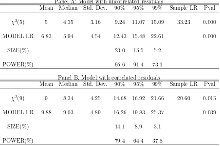
As shown by Bekaert and Hodrick (2001) in the context of the Expectation Hypoth-esis, asymptotic tests such as the LR test can be severely biased in small samples. With the data generated by our bootstrap exercise, we re-estimate the structural model and the unconstrained VAR(1). This yields the small sample distribution of the LR test statistic. As we report in the Panel A of Table 4, there is a considerable size distortion in the LR test of our model. For instance, the 5% critical value is 15.48, instead of the 11.07 asymptotic value, and the empirical size is 15.5%. The top Panel of Figure 8 shows that the empirical distribution of the LR test statistic has a higher mean and a
25Even though the optimal number of lags chosen by the Schwarz criterion is 3 among the unrestricted
VARs, it seems appropriate to compare our model with the nested VAR(1) for the purpose of our study. The impulse responses of an unrestricted VAR(3) are similar to those of the unrestricted VAR(1). Additionally, the right number of lags can be questionable with a small sample size. For instance, the Akaike information criterion selects 15 lags.
26We do not use orthogonalized shocks of the reduced form because the dynamics can be very different
fatter tail than the asymptotic distribution. Unfortunately, the structural model is still strongly rejected. We also bootstrap 1,000 samples under the alternative hypothesis of an unrestricted VAR(1) to calculate the empirical power of the LR test. The empirical power measures the probability of rejecting the null hypothesis when the alternative is true in a small sample. It is calculated as the percentage of LR tests obtained, under the alternative hypothesis, that are lower than a given empirical critical value. For a 5% significance level, the power of the test is 91.4%.
[Insert Table 4 Here]
[Insert Figure 8 Here]
Why is the model so severely rejected? If we visually compare the dynamics implied by the model with the ones of the unrestricted VAR(1), (Panel A of Figure 7), one candidate for the source of rejection seems to be the fact that the model does not reproduce the price puzzle. As mentioned earlier, this is caused by the positive λ, which is, however, what economic theory implies. Below we show that the tight link between the sign of λ
and the price puzzle can be broken if we allow for serial correlation of the error terms. Suppose that the structural errors follow a VAR(1) process:
ǫt+1 =F ǫt+wt+1 (26)
whereF is a 3×3 stationary matrix that captures the structural shock serial correlation and wt+1 is independently and identically distributed with diagonal variance covariance
matrix D. The reduced form solution of the model is still given by (13). The same method of undetermined coefficients can be applied to solve for Ω, Γ and c in terms of
α, A11, B11, B12 and F. It can be shown that the expressions for Ω and c are the same
as equations (15) and (17), and therefore the same methodology for solving the matrix quadratic form, equation (20), can be applied. However, Γ now depends on F:
Γ = (B11−A11Ω) −1
(I+A11ΓF) (27)
Γ can be solved as vec(Γ) = [I3⊗(B11−A11Ω)−(F′⊗A11)]−1vec(I9) where I3 and I9
denote 3×3 and 9×9 identity matrices. In order to estimate this model, we first express the model solution in terms of wt+1 as:
Xt+1 = (I−ΓFΓ −1
)c+ (Ω + ΓFΓ−1
)Xt−ΓFΓ −1
One implication of the Rational Expectations solution of the model with serial cor-relation is that now neither λnor φ govern the direction of the inflation and output gap responses to the monetary policy shock, respectively. This can be seen in equation (28): The coefficient matrices of Xt, Xt−1 and Γ are now functions of F. We first estimate
the model by FIML without any restriction on F. Let Fij be ij-th element of F. Then
zero restrictions on F13, F21, F32 and F33 are imposed because they are not significantly
different from zero. Since the reduced form solution is VAR(2), a natural alternative is an unrestricted VAR(2). These 4 additional restrictions imply that the model has 9 degrees of freedom in total.
In Panel B of Figure 7 we show the reduced form Impulse Response Functions associ-ated with the structural model with autocorrelation. Now the model can reproduce the price puzzle, and the impulse response functions of the model match their unrestricted counterparts very closely. Even though the asymptotic LR test still rejects the model at the 5% level, the rejection is marginal using the small sample LR test (the p-value is 0.039), as is shown in Panel B of Table 4 and the bottom Panel of Figure 8. However, the empirical power of the test is much lower than the one in the original model: The power associated with empirical size of 5% and 1% are 64.4% and 37.8%, respectively. In contrast, the corresponding powers in the model without serial correlation are 91.4% and 73.1%. This evidence suggests that tests of models which imply restricted higher order VARs may suffer from low power against their unrestricted counterparts.
To summarize, even though the model with serial correlation is only marginally re-jected, the original New Keynesian model that we consider remains inconsistent with the data. Our results highlight the need to produce different model specifications, in order to uncover the structural macro relations behind this significant autocorrelation of the residuals.
8
Conclusion
the Fed to deviations of expected inflation from the target since 1979. Our maximum likelihood estimation shows, however, that this result is not statistically significant using linearly and quadratically detrended output. Moreover, our small sample study reveals that the coefficient on expected inflation is upwardly biased. One possibility is that the Taylor rule does not describe accurately the way the Fed conducts monetary policy and that the Fed reacts differently to AS and IS shocks. Further work is necessary to determine whether this is the case.
Appendix
A
Recursive Method
For ease of exposition, we use the mean deviation form of equation (11) in what follows.
B11X¯t=A11EtX¯t+1+B12X¯t−1+ǫt (29)
where ǫt=F ǫt−1+wt and Et−1wt= 0. In this appendix we solve equation (29) forward.
We consider a more general case by allowing the structural errors to follow a VAR(1) process. First we show that there exist sequences of matrices,{Ck,Ωk,Γk, k = 1,2,3, ...}
such that:
¯
Xt =CkEtX¯t+k+1+ ΩkX¯t−1+ Γkǫt
By investigating the properties of the matrices, we propose a solution to the model.
Claim 1 Consider equation (29). Suppose A11, B11, B12, F are real-valued and B11 is
nonsingular. There exist sequences of matrices {Φk,Ψk,Ξk, k = 1,2,3, ...}, which are
functions of A11, B11, B12 and F(thus they are real-valued by construction) such that:
EtX¯t+k = ΦkEtX¯t+k+1+ ΨkX¯t + Ξkǫt (30)
where
Φk+1 = [I−Ψ1Φk] −1
Φ1 (31)
Ψk+1 = [I−Ψ1Φk] −1
Ψ1Ψk (32)
Ξk+1 = [I−Ψ1Φk] −1
[Ψ1Ξk+ Ξ1Fk] (33)
if I−Ψ1Φk is nonsingular for all k.
Proof. Premultiply B−1
11 on both sides of equation (29). Then by shifting one period
forward and taking expectations:
EtX¯t+1 = B −1
11A11EtX¯t+2+B −1
11B12X¯t+B −1 11F ǫt
= Φ1EtX¯t+2+ Ψ1X¯t+ Ξ1ǫt (34)
Suppose EtX¯t+k can be written as follows for some natural number k.
EtX¯t+k= ΦkEtX¯t+k+1+ ΨkX¯t+ Ξkǫt (35)
where Φk, Ψk and Ξk are sequences of matrices of the appropriate dimension. Shift
equation (34) k periods forward and take expectations at time t. Then:
EtX¯t+k+1 = Φ1EtX¯t+k+2+ Ψ1EtX¯t+k+ Ξ1Etǫt+k
= Φ1EtX¯t+k+2+ Ψ1[ΦkEtX¯t+k+1+ ΨkX¯t+ Ξkǫt] + Ξ1Fkǫt (36)
by the law of iterative expectations and from equation (34). Then ifI−Ψ1Φk is invertible
for k:
EtX¯t+k+1= [I−Ψ1Φk] −1
Φ1EtX¯t+k+2+[I−Ψ1Φk] −1
Ψ1ΨkX¯t+[I−Ψ1Φk] −1
[Ψ1Ξk+Ξ1Fk]ǫt
(37)
Therefore Φk+1,Ψk+1, and Ξk+1 are defined as coefficient matrices in this equation, and
these are given by equations (31), (32) and (33).
Claim 2 Consider equation (29) and {Φk,Ψk,Ξk, k= 1,2,3, ...} defined as above. Then
there exist sequences of matrices {Ck,Ωk,Γk, k = 1,2,3, ...} such that:
¯
Xt =CkEtX¯t+k+1+ ΩkX¯t−1+ Γkǫt (38)
Proof. First, expand EtX¯t+1 using equation (30).
EtX¯t+1 = Φ1EtX¯t+2+ Ψ1X¯t+ Ξ1ǫt
= Φ1Φ2EtX¯t+3+ [Φ1Ψ2+ Ψ1] ¯Xt+ [Φ1Ξ2+ Ξ1]ǫt
= Φ1Φ2Φ3EtX¯t+4+ [Φ1Φ2Ψ3+ Φ1Ψ2+ Ψ1] ¯Xt+ [Φ1Φ2Ξ3+ Φ1Ξ2+ Ξ1]ǫt
...
=
k
Y
j=1
ΦjEtX¯t+k+1+ k
X
i=1 i
Y
j=1
Φj−1ΨiX¯t+ k
X
i=1 i
Y
j=1
where Φ0 =I. Therefore equation (29) can be written as:
We can arrange (40) to obtain equation (38), where
Sk =
we define our solution as follows.
Proposition 1 Consider equation (29). Suppose that the sequences of {Sk, Gk,Ωk,Γk}
defined above satisfy the following:
1. Sk, Gk,ΩkandΓkare convergent sequences of matrices: S
are within a unit circle.
is a stationary real-valued bubble-free solution to the structural model (29).
Proof. Since Ω∗
= S∗
and G∗
= Γ∗
F, equations (44) and (45) are the same as (15) and (27), which implies that (46) is a solution to (29). Since all the eigenvalues of Ω∗
are within the unit circle, Ω∗
is stationary. Since all the sequences are real-valued, their limits are real-valued, too. Finally, lim
k→∞CkEt
¯
Xt+k+1 = lim k→∞CkΩ
∗kX¯
t= 0×X¯t = 0 implies that
the solution (46) is bubble-free.
Remark 1 In practice this recursive solution is the same as that obtained through the QZ method in the case of a unique stationary real-valued solution. In the case of multiple solutions it typically corresponds to the solution with the smallest 3 eigenvalues obtained through the QZ method. There is however a nontrivial case where the QZ method gives multiple stationary real valued solutions but none of them coincides with the recursive solution. Suppose there are 2 stable real-valued eigenvalues and one stable complex con-jugate pair arranged in increasing order. The solution associated with the smallest 3 eigenvalues is complex valued. The choice of one of the two real eigenvalues and the complex conjugate pair yields a real-valued solution. Therefore we have 2 real-valued so-lutions. However, neither of them coincides with the recursive solution. In this case, the conditions for the recursive method are not met.27
B
Uniqueness of the solution
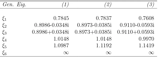
Table 5 shows the generalized eigenvalues associated with the three FIML estimated sets of parameters. As explained in section 4.2, in the first two specifications (with output linearly and quadratically detrended), we have a unique solution, since there are exactly 3 eigenvalues less than unity, the same number as predetermined state variables in the model. We also verified that the recursive solution coincides with the one obtained through the QZ method.
[Insert Table 5 Here]
For the third specification (with output detrended using the CBO measure), we have multiple solutions, since there are 4 eigenvalues less than 1 in moduli. Our recursive
27Notice that our recursive method is different from that of Binder and Pesaran (1997) in the sense
method converges to the QZ solution with the first 3 eigenvalues. In general, we found that, holding the remaining parameters at their estimated values in column (1) of Table 2, when λ is positive, the solution is unique. For negative values of λ, large in absolute value, there is no real valued solution. For small negative values of λ, as estimated with the CBO measure, there are multiple solutions. The dynamics implied by our recursive solution for this case are shown in the sensitivity analysis with λ=−0.0014.
C
Bootstrap Analysis
Our structural model and the unrestricted VAR(1) can be expressed respectively as:
Xt = c+ ΩXt−1+ Γǫt (47)
Xt = d+ ΘXt−1+ut (48)
where V ar(Γǫt) = ΓDΓ ′
and V ar(ut) = Υ. If the structural model is true, it should be
the case that ΓDΓ′
= Υ. We orthogonalize the unrestricted VAR(1) error terms through a Choleski decomposition, so that V ar(ut) = E(utu′t) = Υ = CC
′
, where C is lower triangular. Therefore, ut =Cζt, where ζt has mean zero and ones in the diagonal of its
variance covariance matrix. The unrestricted VAR(1) can then be expressed as:
Xt=d+ ΘXt−1+Cζt (49)
Under the null of the modelǫt=
√
Dξt, whereξthas mean zero and ones in the diagonal
of its variance covariance matrix. The model can then be expressed as:
Xt=c+ ΩXt−1+ Γ
√
Dξt (50)
Therefore, if the model is true it should be the case that Γ√D=Cand thatV ar(Γ√Dξt) =
V ar(Cζt). We perform a bootstrap analysis under the null of the structural model and
under the alternative data generating process, the VAR(1). Under the null we proceed as follows:
1. We bootstrap the unconstrained errors, ut, with replacement.
along with theζt disturbances, which are obtained by pre-multiplying theuterrors
by C−1
. For every sample we discard the first 500 data points and retain the last 78 observations to have the same size as the original data set.
3. We re-estimate both the model and the unrestricted VAR(1) 1,000 times. This yields 1,000 parameter sets and 1,000 LR tests.
With the 1,000 parameter sets, we obtain the small sample distribution of the structural parameters under the null of the model. To compute the empirical critical values of the LR test statistic, we select the corresponding quantiles of the empirical distribution of the LR test statistic. The bootstrap simulations under the alternative hypothesis differ from the ones under the null in that, in step 2, the data sets are constructed conditional on d
and Θ, instead ofc, Ω andD. The power of the test is calculated as the percentage of LR tests obtained, under the alternative hypothesis, which is lower than a given empirical significance level.
References
Amato, Jeffery, and Thomas Laubach, 1999, Monetary Policy In An Estimated Optimization-Based Model With Sticky Prices And Wages, Federal Reserve Bank of Kansas City, Research Working Paper 99-09.
Bai, Jushan, Robin L. Lumsdaine, and James H. Stock, 1998, Testing for and dating breaks in stationary and nonstationary multivariate time series, Review of Economic Studies 65, 395–432.
Bekaert, Geert, Campbell R. Harvey, and Robin L. Lumsdaine, 2002, Dating the inte-gration of world equity markets, Journal of Financial Economics 65, 203–247.
Bekaert, Geert, and Robert J. Hodrick, 2001, Expectation Hypotheses Tests, Journal of Finance 56, 1357–1392.
Bekaert, Geert, Robert J. Hodrick, and David A. Marshall, 1997, On biases in tests of the Expectations Hypotheses of the term structure of interest rates,Journal of Financial Economics 44, 309–348.
Binder, Michael, and M. Hashem Pesaran, 1997, Multivariate Linear Rational Expecta-tions Models: Characterization of the Nature of the SoluExpecta-tions and Their Fully Recur-sive Computation,Econometric Theory 13, 877–888.
Blanchard, Olivier J., and C.M. Kahn, 1980, The Solution of Linear Difference Models Under Rational Expectations, Econometrica 48, 1305–1311.
Blanchard, Olivier J., and D. Quah, 1989, The Dynamic Effects of Aggregate Demand and Supply Disturbances, American Economic Review 79, 655–673.
Boivin, Jean, and Marc Giannoni, 2003, Has Monetary Policy Become More Effective?,
Mimeo, Columbia University.
Boivin, Jean, and Mark Watson, 1999, Time-Varying Parameter Estimation in the Linear IV Framework, Mimeo, Princeton University.
Christiano, L., M. Eichenbaum, and C. Evans, 1999, Monetary Policy Shocks: What have we learned and to what end? in John B. Taylor and Michael Woodford, Eds.,
Christiano, L., M. Eichenbaum, and C. Evans, 2001, Nominal Rigidities and the Dynamic effects of a shock to Monetary Policy, NBER Working Paper No 8403.
Clarida, Richard H., Jordi Gal´ı, and Mark Gertler, 1999, The Science of Monetary Policy: A New Keynesian Perspective, Journal of Economic Literature 37, 1661–1707.
Clarida, Richard H., Jordi Gal´ı, and Mark Gertler, 2000, Monetary Policy Rules and Macroeconomic Stability: Evidence and some Theory,Quarterly Journal of Economics
115, 147–180.
Estrella, Arturo, and Jeffrey Fuhrer, 1999, Are Deep Parameters Stable? The Lucas Critique as an Empirical Hypothesis, Working Paper.
Feldstein, Martin, 1994, American Economic Policy in the 1980’s: A personal view in Martin Feldstein, Ed., American Economic Policy in the 1980’s, The University of Chicago Press, pp. 1–79.
Fuhrer, Jeffrey C., 2000, Habit Formation in Consumption and Its Implications for Monetary-Policy Models, American Economic Review 90, 367–389.
Fuhrer, Jeffrey C., and George Moore, 1995, Inflation Persistence, Quarterly Journal of Economics 440, 127–159.
Gal´ı, Jordi, and Mark Gertler, 1999, Inflation Dynamics,Journal of Monetary Economics
44, 195–222.
Ireland, Peter, 2001, Sticky-Price Models of the Business Cycle: Specification and Sta-bility, Journal of Monetary Economics 47, 3–18.
Leeper, Eric M., Christopher Sims, and Tao Zha, 1996, What does Monetary Policy do?,
Brooking Papers on Economic Activity 2, 1–63.
Leeper, Eric M., and Tao Zha, 2000, Assessing Simple Policy Rules: A View from a Complete Macro Model,Federal Reserve Bank of Atlanta. Working Paper 19.
McCallum, Bennett T., 1983, On Non-Uniqueness in Rational Expectations Models: An Attemp at Perspective,Journal of Monetary Economics 11, 139–168.
McCallum, Bennett T., 2001, Should Monetary Policy Respond Strongly to Output Gaps,
NBER Working Paper No 8225.
McCallum, Bennett T., and Edward Nelson, 1998, Performance of Operational Policy Rules in an Estimated Semi-Classical Structural Model in John B. Taylor, Ed., Mon-etary Policy Rules, Chicago: University of Chicago Press, pp. 15–45.
Roberts, John, 1995, New Keynesian Economics and the Phillips Curve, Journal of Money, Credit and Banking 37, 975–984.
Rotemberg, Julio J., and Michael Woodford, 1998, An Optimization-Based Econometric Framework for the Evaluation of Monetary Policy: Expanded Version,NBER Working Paper No T0233.
Rudebusch, Glenn D., 2002, Assessing Nominal Income Rules for Monetary Policy with Model and Data Uncertainty,Economic Journal 112, 402–432.
Rudebusch, Glenn D., and Lars E. O. Svensson, 1999, Policy Rules for Inflation Targeting in John B. Taylor, Ed., Monetary Policy Rules Chicago: University of Chicago Press, pp. 203–262.
Smets, Frank, 2000, What horizon for price stability, ECB Working Paper 24.
Smets, Frank, and Raf Wouters, 2001, Monetary Policy in an Estimated Dynamic General Equilibrim Model of the Euro Area, Mimeo.
Taylor, John B., 1999, A Historical Analysis of Monetary Policy Rules in John B. Taylor, Ed., Monetary Policy Rules, Chicago: University of Chicago Press, pp. 319–341.
Uhlig, Harald, 1997, A Toolkit for Analyzing Nonlinear Dynamic Stochastic Models Easily in Ram´on Marim´on and Andrew Scott , Ed., Computational Methods for the Study of Dynamic Economies, Oxford Universtiy Press, pp. 30–61.
Table 1: Sup-Wald Break Date Statistics
Sample Period VAR Sup-Wald Break Date 90% Confidence Interval
1954:3Q-2000:1Q 1 72.02 1980:4Q 1980:3Q-1981:1Q
1954:3Q-2000:1Q 2 103.33 1980:4Q 1980:3Q-1981:1Q
1954:3Q-2000:1Q 3 116.86 1980:4Q 1980:3Q-1981:1Q
Table 2: FIML Estimates and Small Sample Distribution of the Structural Parameters of the Model
Parameters (1) (2) (3) (4) (5) (6)
δ 0.5586 0.5585 0.5681 [0.5256 0.5915] 0.5764 [0.5239 0.6565] (0.0168) (0.0173) (0.0248)
λ 0.0011 0.0011 -0.0002 [-0.0010 0.0032] 0.0028 [-0.0034 0.0131] (0.0011) (0.0011) (0.0014)
µ 0.4859 0.4810 0.4801 [0.4195 0.5523] 0.4826 [0.2386 0.5728] (0.0339) (0.0358) (0.0376)
φ 0.0045 0.0054 0.0065 [-0.0055 0.0146] 0.0140 [-0.0065 0.0760] (0.0051) (0.0056) (0.0057)
ρ 0.8458 0.8419 0.8767 [0.7441 0.9475] 0.8148 [0.6629 0.9211] (0.0519) (0.0415) (0.0404)
β 1.6409 1.6413 2.1506 [0.1267 3.1551] 1.9027 [0.3983 5.0267] (0.7725) (0.4487) (0.5058)
γ 0.6038 0.6126 1.0079 [-0.2086 1.4161] 0.6214 [-0.3402 1.7680] (0.4145) (0.3163) (0.4648)
σAS 0.4585 0.4588 0.4661 [0.3809 0.5361] 0.4635 [ 0.3956 0.5344]
(0.0396) (0.0389) (0.0429)
σIS 0.3734 0.3766 0.3570 [0.3096 0.4372] 0.3841 [0.2996 0.5553]
(0.0326) (0.0341) (0.0330)
σM P 0.7327 0.7305 0.7281 [0.6239 0.8416] 0.7105 [0.5399 0.8818]
(0.0555) (0.0588) (0.0586)