Full Terms & Conditions of access and use can be found at
http://www.tandfonline.com/action/journalInformation?journalCode=ubes20
Download by: [Universitas Maritim Raja Ali Haji] Date: 12 January 2016, At: 23:03
Journal of Business & Economic Statistics
ISSN: 0735-0015 (Print) 1537-2707 (Online) Journal homepage: http://www.tandfonline.com/loi/ubes20
Comparing Density Forecasts via Weighted
Likelihood Ratio Tests
Gianni Amisano & Raffaella Giacomini
To cite this article: Gianni Amisano & Raffaella Giacomini (2007) Comparing Density Forecasts via Weighted Likelihood Ratio Tests, Journal of Business & Economic Statistics, 25:2, 177-190, DOI: 10.1198/073500106000000332
To link to this article: http://dx.doi.org/10.1198/073500106000000332
Published online: 01 Jan 2012.
Submit your article to this journal
Article views: 373
View related articles
Comparing Density Forecasts via Weighted
Likelihood Ratio Tests
Gianni AMISANO
Department of Economics, University of Brescia, Brescia, Italy (amisano@eco.unibs.it)
Raffaella GIACOMINI
Department of Economics, University of California, Los Angeles, CA 90095-1477 (giacomin@econ.ucla.edu)
We propose a test for comparing the out-of-sample accuracy of competing density forecasts of a variable. The test is valid under general conditions: The data can be heterogeneous and the forecasts can be based on (nested or nonnested) parametric models or produced by semiparametric, nonparametric, or Bayesian estimation techniques. The evaluation is based on scoring rules, which are loss functions defined over the density forecast and the realizations of the variable. We restrict attention to the logarithmic scoring rule and propose an out-of-sample “weighted likelihood ratio” test that compares weighted averages of the scores for the competing forecasts. The user-defined weights are a way to focus attention on different regions of the distribution of the variable. For a uniform weight function, the test can be interpreted as an extension of Vuong’s likelihood ratio test to time series data and to an out-of-sample testing framework. We apply the tests to evaluate density forecasts of U.S. inflation produced by linear and Markov-switching Phillips curve models estimated by either maximum likelihood or Bayesian methods. We conclude that a Markov-switching Phillips curve estimated by maximum likelihood produces the best density forecasts of inflation.
KEY WORDS: Loss function; Predictive ability testing; Scoring rules.
1. INTRODUCTION
A density forecast is an estimate of the future probability dis-tribution of a random variable, conditional on the information available at the time the forecast is made. It, thus, represents a complete characterization of the uncertainty associated with the forecast, as opposed to a point forecast, which provides no information about the uncertainty of the prediction.
Density forecasting is receiving increasing attention in both macroeconomics and finance (see Tay and Wallis 2000 for a survey). A famous example of density forecasting in macro-economics is the “fan chart” of inflation and gross domestic product (GDP) published by the Bank of England and by the Sveriges Riksbank in Sweden in their quarterly inflation reports (for other examples of density forecasting in macroeconomics, see also Diebold, Tay, and Wallis 1999; Clements and Smith 2000). In finance, where the wide availability of data and the in-creasing computational power make it possible to produce more accurate estimates of densities, the examples are numerous. Leading cases are in risk management, where forecasts of port-folio distributions are issued with the purpose of tracking mea-sures of portfolio risk such as the value at risk (see, e.g., Duffie and Pan 1996) or the expected shortfall (see, e.g., Artzner, Delbaen, Elber, and Heath 1997). Another example is the ex-traction of density forecasts from option price data (see, e.g., Soderlind and Svensson 1997). The vast literature on forecast-ing volatility with GARCH-type models (see Bollerslev, Engle, and Nelson 1994) and its extensions to forecasting higher mo-ments of the conditional distribution (see Hansen 1994) can also be seen as precursors to density forecasting. The use of sophis-ticated distributions for the standardized residuals of a GARCH model and the modeling of time dependence in higher moments is in many cases an attempt to capture relevant features of the data to better approximate the true distribution of the variable. Finally, in the multivariate context, a focus on densities is the
central issue in the literature on copula modeling and forecast-ing, which is gaining interest in financial econometrics (Patton 2006).
With density forecasting becoming more and more wide-spread in applied econometrics, it is necessary to develop re-liable techniques to evaluate the forecasts’ performance. The literature on evaluation of density forecasts (or, equivalently, predictive distributions) is still young, but growing at a fast speed. In one of the earliest contributions, Diebold, Gunther, and Tay (1998) suggested evaluating a sequence of density fore-casts by assessing whether the probability integral transforms of the realizations of the variable with respect to the forecast den-sities are independent and identically distributed (iid) U(0,1). Whereas Diebold et al. (1998) adopted mainly qualitative tools for testing the iid U(0,1)behavior of the transformed data, for-mal tests of the same hypothesis were suggested by Berkowitz (2001), Hong and White (2005), and Hong (2000). Tests that account for parameter estimation uncertainty were proposed by Hong and Li (2005), Bai (2003), and Corradi and Swanson (2006a) (the latter further allowing for dynamic misspecifica-tion under the null hypothesis).
It is important to emphasize that the preceding methods fo-cus on absolute evaluation, that is, on evaluating the “good-ness” of a given sequence of density forecasts, relative to the data-generating process. In practice, however, it is likely that any econometric model used to produce the sequence of den-sity forecasts is misspecified, and an absolute test will typically give no guidance to the user as to what to do in case of rejection. In this situation, a more practically relevant question is how to decide which of two (or more) competing density forecasts is preferable, given a measure of accuracy. The comparative
© 2007 American Statistical Association Journal of Business & Economic Statistics April 2007, Vol. 25, No. 2 DOI 10.1198/073500106000000332
177
evaluation of density forecasts has been relatively less ex-plored in the literature. A number of empirical works have con-sidered comparisons of density forecasts (e.g., Clements and Smith 2000; Weigend and Shi 2000), but they have predomi-nantly relied on informal assessments of predictive accuracy. More recently, Corradi and Swanson (2005, 2006b) proposed a bootstrap-based test for evaluating multiple misspecified pre-dictive models, based on a generalization of the mean squared error.
In this article we contribute to the literature about compar-ative evaluation of density forecasts by proposing formal out-of-sample tests for ranking competing density forecasts that are valid under very general conditions. Our method is an alterna-tive approach to Corradi and Swanson (2005, 2006b), because it uses a different measure of accuracy, and is further valid under more general data and estimation assumptions.
We consider the situation of a user who is interested in com-paring the out-of-sample accuracy of two competingforecast methods, where we define the forecast method to be the set of choices that the forecaster makes at the time of the predic-tion, including the density model, the estimation procedure, and the estimation window. We impose very few restrictions on the forecast methods. The density forecasts can be based on para-metric models, either nested or nonnested, whose parameters are known or estimated. The forecasts could be further pro-duced using semiparametric, nonparametric, or Bayesian esti-mation techniques. As in Giacomini and White (2006), the key requirement is that the forecasts are based on a finite estima-tion window. This assumpestima-tion is motivated by our explicit al-lowance for a data-generating process that may change over time (unlike all of the existing literature, which assumes sta-tionarity), a likely feature of the series that economists forecast (Clements and Hendry 1999). The idea is that, in the presence of instability, observations at the beginning of the sample at some point become uninformative and one should rather base fore-casts on a window containing only the most recent data points. For this reason, we focus our attention on forecasts produced by a rolling-window forecasting scheme (although a fixed fore-casting scheme is also allowed). A further motivation for the finite estimation window assumption is that it is a convenient way to create an environment with asymptotically nonvanishing estimation uncertainty. As explained in Giacomini and White (2006), this seems appropriate in forecasting contexts because it involves comparing the accuracy of the forecasting models, while at the same time taking into account the possibly different amounts of estimation uncertainty contained in each forecast. It also turns out that this feature of the asymptotic framework of Giacomini and White (2006) makes it more generally ap-plicable than previous frameworks (e.g., West 1996), for exam-ple, allowing comparison of forecasts based on both nested and nonnested models.
We follow the literature on probability forecast evaluation and measure the relative performance of the density forecasts using scoring rules, which are loss functions defined over the density forecast and the outcome of the variable. We restrict at-tention to the logarithmic scoring rule, which has an intuitively appealing interpretation and is mathematically convenient. We consider the out-of-sample performance of the two forecasts and rank them according to the relative magnitude of a weighted
average of the logarithmic scores over the out-of-sample period. Our weighted likelihood ratio (WLR) test establishes whether such weighted averages are significantly different from each other. The use of weights gives our tests flexibility by allowing the user to compare the performance of the density forecasts in different regions of the distribution of the variable, distinguish-ing, for example, predictive ability in “normal” periods from that in “extreme” periods. In the equal-weights case, our test is related to Vuong’s (1989) likelihood ratio test for nonnested hypotheses, the differences being that (1) we compare forecast methods rather than models, (2) we allow the underlying mod-els to be either nested or nonnested, (3) we perform the eval-uation out of sample rather than in sample, and (4) we allow the data to be heterogeneous and dependent rather than iid. Fi-nally, it is important to note that, as in Giacomini and White (2006), a distinguishing feature of our null hypothesis is that it is stated in terms of parameter estimates rather than population parameter values.
We conclude with an application comparing the performance of density forecasts produced by a linear Phillips curve model of inflation versus a Markov-switching Phillips curve, estimated by either maximum likelihood or Bayesian methods. The fo-cus on the density forecast—rather than the point forecast— performance of Markov-switching versus linear models of inflation is empirically relevant and can shed new light on the relative forecast accuracy of linear and nonlinear models be-cause the two models imply different densities for inflation (a mixture of normals for the Markov-switching versus a nor-mal density for the linear model).
Our article is organized as follows. Section 2 describes the notation and the testing environment, Section 3 introduces the loss functions, and Section 4 introduces our weighted likeli-hood ratio test. Section 5 contains a Monte Carlo experiment investigating the empirical size and power properties of our test. In Section 6 we apply our tests to the evaluation of competing density forecasts of inflation obtained by a Markov-switching or a linear Phillips curve model, estimated by either classical or Bayesian methods. Section 7 concludes. The proofs are given in Appendix B.
2. DESCRIPTION OF THE ENVIRONMENT
Consider a stochastic process Z ≡ {Zt:→Rs+1,s∈N, tion set at timet and suppose that two competing models are used to produce one-step-ahead density forecasts of the vari-able of interest,Yt+1,using the information inFt. Denote the forecasts by fˆm,t ≡f(Zt,Zt−1, . . . ,Zt−m+1; ˆβm,t) and gˆm,t ≡
g(Zt,Zt−1, . . . ,Zt−m+1; ˆβ
m,t), wheref andg are measurable functions. The subscripts indicate that the time-tforecasts are measurable functions of themmost recent observations, where
mis finite.
Thek×1 vectorβˆm,t collects the parameter estimates from both models. Note that the only requirement that we impose on how the forecasts are produced is that they are measurable func-tions of a finite estimation window. In particular, this allows the
forecasts to be produced by parametric as well as semiparamet-ric, nonparametsemiparamet-ric, or Bayesian estimation methods.
We perform the out-of-sample evaluation using a “rolling window” estimation scheme. Let T be the total sample size. The first one-step-ahead forecasts are produced at timem, us-ing data indexed 1, . . . ,m, and they are compared toYm+1. The
estimation window are then rolled forward one step and the second forecasts are obtained using observations 2, . . . ,m+1, and they are compared to Ym+2. This procedure is thus
it-erated, and the last forecasts are obtained using observations
T−m, . . . ,T−1, and they are compared toYT.This yields a sequence ofn≡T−mout-of-sample density forecasts.
Note that the condition thatmbe finite rules out an expand-ing estimation window forecastexpand-ing scheme. This condition is, however, compatible with a fixed estimation sample forecast-ing scheme, where allnout-of-sample forecasts depend on the same parameters estimated once on the firstmobservations. For clarity of exposition, we hereafter restrict attention to a rolling-window forecasting scheme but all the results remain valid for a fixed estimation sample scheme.
All of the above elements—the model, the estimation meth-od, and the size of the estimation window—constitute what we call the “forecast method,” which is the object of our evaluation.
3. LOSS FUNCTIONS AND DENSITY FORECASTING
The incorporation of loss functions into the forecasting prob-lem has until now focused on the definition of classes of loss functions of the formL(fˆt,τ,Yt+τ), whereˆft,τ is aτ-step-ahead
point forecast of Yt+τ. In the vast majority of cases, the loss
function is assumed to depend only on the forecast error, as for quadratic loss or general asymmetric loss (e.g., Christoffersen and Diebold 1997; Weiss 1996). Weiss (1996) showed that, in this framework, the optimal predictor is some summary mea-sure of the true conditional density of the variable Yt+τ (the
mean for quadratic loss, the median for absolute error loss, etc.). This means that a user with, say, a quadratic loss function is only concerned with the accuracy of the mean prediction and will be indifferent to density forecasts that yield the same fore-cast for the conditional mean. The discussion of loss functions relevant for density forecasting must, thus, involve a shift of focus.
Because a density forecast can be seen as a collection of probabilities assigned by the forecaster to all attainable events, the tools developed in the probability forecasting evaluation lit-erature can be readily employed. In particular, we will make use of so-called scoring rules (see, e.g., Winkler 1967; Diebold and Lopez 1996; Lopez 2001), which are loss functions whose ar-guments are the density forecast and the actual outcome of the variable. We restrict our attention to the logarithmic scoring rule
S(f,Y)=logf(Y),whereY is the observed value of the vari-able andf(·) the density forecast. Intuitively, the logarithmic score rewards a density forecast that assigns high probability to the event that actually occurred. The logarithmic score is also mathematically convenient, being the only scoring rule that is solely a function of the value of the density at the realization of the variable.
When a sequence of competing density forecasts and of re-alizations of the variable is available, one can rank the density
forecasts by comparing their average scores. Forf andg intro-duced in Section 2, one would compute the average logarithmic scores over the out-of-sample period,n−1Tt=−m1logˆfm,t(Yt+1)
andn−1Tt=−m1loggˆm,t(Yt+1),and select the forecast yielding
the highest score. We further consider the possibility of com-paringweighted averages of the logarithmic scores, which al-lows the forecaster to put greater weight on particular regions of the distribution of the variable. For example, one may be particularly interested in predicting “tail events,” as these could lead to different investment strategies. Another situation of in-terest might be predicting events that fall near the center of the distribution, as a way to ignore the influence of possi-ble outliers on predictive performance. Finally, one may want to focus on predictive performance in the right or in the left tail of the distribution, as in the case of forecasting mod-els for risk management, where losses have different implica-tions than gains. For each of the preceding situaimplica-tions, we can define an appropriate weight function w(·) and compare the weighted average scores n−1Tt=−m1w(Yt+1)logfˆm,t(Yt+1)and
n−1Tt=−m1w(Yt+1)loggˆm,t(Yt+1). The weight functionw(·)can be arbitrarily chosen by the forecaster to select the desired re-gion of the distribution ofYt. The only requirement imposed on the weight function is that it be positive and bounded. For exam-ple, when the data have unconditional mean 0 and variance 1, one could consider the following weights:
• Center of distribution:w1(Y)=φ (Y), φstandard normal density function (or pdf )
• Tails of distribution:w2(Y)=1−φ (Y)/φ (0), φstandard normal pdf
• Right tail:w3(Y)=(Y), standard normal distribution function (or cdf )
• Left tail:w4(Y)=1−(Y), standard normal cdf.
A formal test for comparing the (weighted) average logarith-mic scores is proposed in the following section.
4. WEIGHTED LIKELIHOOD RATIO TESTS
For a given weight functionw(·)and two alternative condi-tional density forecastsf andgforYt+1, let
WLRm,t+1≡w(Ytst+1)
logfˆm,t(Yt+1)−loggˆm,t(Yt+1)
, (1)
where Ytst+1 ≡(Yt+1 − ˆµm,t)/σˆm,t is the realization of the variable at timet+1, standardized using estimates of the un-conditional mean and standard deviation ofYt,µˆm,t andσˆm,t,
computed on the same sample on which the density forecasts are estimated. A test for equal performance of density forecasts
f andgcan be formulated as a test of the null hypothesis
H0:E[WLRm,t+1] =0, t=1,2, . . . against, (2)
HA:E[WLRm,n] =0 for allnsufficiently large, (3) whereWLRm,n=n−1tT=−m1WLRm,t+1. Note that, as in
Giaco-mini and White (2006), our null hypothesis is different from that considered in the literature on model selection testing (e.g., Vuong 1989) in that it depends on parameter estimates rather than on population values. Also note that our formulation of the null and alternative hypotheses reflects the fact that we do not
impose the requirement of stationarity of the data. We call a test ofH0a weighted likelihood ratio test.
Our test is based on the statistic
tm,n=
WLRm,n ˆ
σn/√n
, (4)
where σˆn2 is a heteroscedasticity and autocorrelation con-sistent (HAC) estimator of the asymptotic variance σn2 =
var[√n WLRm,n]: West 1987; Andrews 1991 for discussion). In practice, it is of-ten the case that short truncation lags pn improve the finite-sample properties of tests of equal predictive ability (Diebold and Mariano 1995), which motivates our choice ofpn=0 for the Monte Carlo experiment in Section 5 and for the empirical application in Section 6.
A level α test rejects the null hypothesis of equal perfor-mance of forecastsfandgwhenever|tm,n|>zα/2, wherezα/2is
the(1−α/2)quantile of a standard normal distribution. In case of rejection, one would choosef ifWLRm,nwere positive andg ifWLRm,nwere negative. The following theorem provides the asymptotic justification for our test.
Theorem 1(Weighted likelihood ratio test). For a given es-timation window size m<∞ and a weight function w(·),
1. Note that we do not require stationarity of the underly-ing data-generatunderly-ing process. Instead, assumption 1 allows the data to be characterized by heterogeneity and depen-dence, in particular, permitting structural changes at un-known dates.
2. Assumption 2 requires the existence of at least four mo-ments of the log-likelihoods, as functions of estimated pa-rameters. The plausibility of this requirement depends on the models, the underlying data-generating process, and the estimators on which the forecasts may depend; thus, it should be verified on a case-by-case basis. For example, for normal density forecasts, this assumption imposes the
existence of at least eight moments of the variable of in-terest and the existence of the finite-sample moments of the conditional mean and variance estimators.
3. As in Giacomini and White (2006), we derive our test using an asymptotic framework where the number of out-of-sample observations n goes to ∞, whereas the estimation sample size m remains finite. Besides being motivated by the presence of underlying heterogeneity, the use of finite-masymptotics is a way to create an envi-ronment with asymptotically nonvanishing estimation un-certainty.
4. Assumption 3 requires the asymptotic variance to be pos-itive as the sample size grows. In conventional asymp-totic frameworks (e.g., West 1996), this assumption could be violated when comparing forecasts from nested mod-els. In our framework, instead, the presence of asymptot-ically nonvanishing estimation uncertainty, ensures that assumption 3 is not violated and, thus, makes our tests applicable to both nested and nonnested models.
5. For the casew(·)=1, the weighted likelihood ratio test is related to Vuong’s (1989) likelihood ratio test for nonnested hypotheses. In that case, (1) the objects of com-parison are competing nonnested models, (2) the evalua-tion is performed in sample, and (3) the data are assumed to be independent and identically distributed. In contrast, in this article, (1) we evaluate competing forecast methods (i.e., not only models but also estimation procedures and estimation windows), where the underlying models can be either nested or nonnested; (2) we perform the evaluation out of sample; and (3) we allow the data to be character-ized by heterogeneity and dependence.
The preceding weighted likelihood ratio test is conditional on a particular choice of weight function. To reduce dependence on the functional form chosen for the weight function, one might consider generalizing the test (1) to take into account possibly different specifications forw(·). For example, if the null hy-pothesis of equal performance is rejected in favor of, say, den-sity forecastf,a test of superior predictive ability off relative togcould be constructed by considering a sequence ofJweight functions{wj(·)}Jj=1spanning the whole support of the uncondi-tional distribution ofYt+1and testing whetherE[WLRm,n] =0 for allwj.The theoretical underpinnings of such a test are not considered further in this article and are left for future research.
5. MONTE CARLO EXPERIMENT
In this section we analyze the finite-sample properties of our test in samples of the sizes typically available in macroeco-nomic applications. The design of the Monte Carlo experiment poses problems because the null hypothesis depends on esti-mated parameters, which makes it arduous to ensure that dif-ferent models yield equally accurate density forecasts for each Monte Carlo replication. Nonetheless, for the case w(y)=1 and when the forecasts are normal densities with different con-ditional mean specifications, we are able to generate data that satisfy the null hypothesis by exploiting the following result.
Proposition 2. Letfˆm,t=N(µˆfm,t,1)andgˆm,t=N(µˆgm,t,1). If E[Yt+1|Ft] = (µˆfm,t + ˆµ
g
m,t)/2, then E[logfˆm,t(Yt+1) − loggˆm,t(Yt+1)] =0.
Data that satisfy the null are then obtained by first construct-ing forecasts{ ˆfm,t,gˆm,t},fˆm,t=N(µˆ1t,1)andgˆm,t=N(µˆ2t,1), for Yt+1 and then redefining the series as Yt+1 =(µˆfm,t +
ˆ
µgm,t)/2+εt+1, εt+1∼iid N(0,1). To create data characterized
by realistic heterogeneous behavior, and to remain as close as possible to the empirical application, we letYtbe U.S. inflation, measured as the log difference of the monthly consumer price index. We then consider competing density forecasts based ei-ther on a Phillips curve model of inflation or on a random-walk model for the consumer price index. This comparison is of em-pirical interest, because it reflects the common practice of com-paring forecasts based on some economically plausible model to forecasts based on a simple, atheoretical benchmark model. A further motivation for our Monte Carlo design is our desire to capture the effect of estimation uncertainty on forecast per-formance, which could be important when the two models have different numbers of parameters. To this end, we utilize Propo-sition 2 to ensure that the two models yield equally accurate forecasts, while at the same time accounting for the differ-ent amounts of estimation uncertainty contained in each fore-cast. Our focus on estimation uncertainty further motivates our choice of different conditional mean specifications (as opposed to, say, different density functions) in producing the competing forecasts, given that in macroeconomic applications any estima-tion uncertainty in the density forecasts is likely to come from estimation of conditional mean parameters.
We proceed as follows. For a givenm,we constructµˆfm,tand
whereuis monthly U.S. unemployment and the parameters are estimated using data(Yt, . . . ,Yt−m+1).We consider a number
of in-sample and out-of-sample sizes m=(25,50,100,150)
andn=(50,100,150), and for each (m,n)pair we generate 5,000 Monte Carlo replications of the series {Yt+1,fˆm,t,gˆm,t} using a rolling-window forecasting scheme on the sample of size m+n ending with the observations for May 2004. For each iteration, we evaluate the densities atYt+1 and compute
the score difference logfˆm,t(Yt+1)−loggˆm,t(Yt+1). The
recur-sion generatesnscore differences, which we utilize to compute the test statistic (4). We then compute the proportion of rejec-tions of the null hypothesisH0at the 5% nominal level, using
the test of Theorem 1. The empirical size of the test is reported in Table 1, which shows that the test has good size properties, even for sample sizes as small as 50 total observations.
We next investigate the power of the weighted likelihood ra-tio test against the alternative hypothesis that WLRm,t+1 has
nonzero mean: of values for WLRm,n obtained in our empirical application (Table 3A). For each(n,c)pair and for each replication, we
Table 1. Size of Nominal .05 Test
n
m 25 50 100 150
25 .051 .053 .049 .050
50 .054 .054 .050 .047
100 .053 .054 .044 .057
150 .059 .051 .054 .054
NOTE: The table reports the empirical size of the test of Theorem 1. Entries repre-sent the rejection frequencies over 5,000 Monte Carlo replications of the null hypothesis
H0:E[ logˆfm,t(Yt+1)−loggˆm,t(Yt+1)]=0, where the density forecastsf andgand the
data-generating process are defined in Section 5. The nominal size is .05. Each cell corresponds to a pair of in-sample and out-of-sample sizes (m,n).
generate data under the alternative hypothesis by first construct-ing the conditional mean forecastsµˆfm,tandµˆgm,t as in (5) and
jections of the null hypothesis at the 5% nominal level using the weighted likelihood ratio test.
The test displays good power properties, provided the sample size is large enough(n≥150). It, thus, appears that our test is best suited for financial and macroeconomic applications where data are available at least at monthly frequency.
6. DENSITY FORECASTS OF INFLATION FROM LINEAR AND MARKOV–SWITCHING
PHILLIPS CURVES
6.1 Motivation
A key framework for forecasting inflation is the Phillips curve (henceforth, PC), a model relating inflation to some measure of the level of real activity, in most cases the unem-ployment rate. Stock and Watson (1999) investigated the point forecasting accuracy of the PC, comparing it to that of com-peting models, such as simple autoregressions and multivari-ate models. In this study the Phillips curve is found to produce more accurate forecasts than competing models, particularly when the activity variable is carefully chosen. Another inter-esting finding is the presence of parameter variation across dif-ferent subsamples.
We follow Stock and Watson (1999) in considering the PC as a reference for our analysis and contribute to the literature as-sessing its forecast performance in several ways. First, we eval-uate the accuracy of density forecasts rather than point forecasts
Table 2. Power of Test
n
NOTE: The table reports the rejection frequencies over 5,000 Monte Carlo replications of the null hypothesisH0:E[ logˆfm,t(Yt+1)−loggˆm,t(Yt+1)]=0 using the test of Theorem 1. The density
forecastsfandgand the data-generating process are defined in Section 5. The in-sample size ism=100.nis the out-of-sample size andc=E[ logfˆm,t(Yt+1)−loggˆm,t(Yt+1)].
and compare a linear PC specification to an alternative specifi-cation that allows for Markov switching (henceforth MS) of its parameters. We choose the MS model as a credible competitor to the linear PC model both because the MS mechanism allows for parameter variation over the business cycle and because the predictive distribution generated by the MS model is non-Gaussian, which is of potential interest when comparing density forecast performance. Our second contribution is the evaluation of the impact on forecast performance of using different esti-mation techniques when producing the forecasts. In particular, we consider estimating both the linear and the MS model by either classical or Bayesian methods. Note that a formal com-parison of these forecast methods could not be conducted us-ing previously available techniques, because they do not easily accommodate nested model comparisons and Bayesian estima-tion. This application, thus, gives a flavor of the generality of the forecasting comparisons that can be performed using our testing framework.
6.2 Linear and Markov-Switching Phillips Curves
Following Stock and Watson (1999), our linear model is a PC model in which changes of inflation depend on their lags and on lags of the unemployment rate:
πt=α+β(L)πt+γ (L)ut+σ·εt, whereCPIt is the consumer price index and ut is the unem-ployment rate. This specification is consistent with the “nat-ural rate hypothesis,” because the nat“nat-ural rate of unemployment (NAIRU) isu∗= −α/γ (1). Note that we implicitly assume that
πtandutdo not have a unit root, which is confirmed by ADF tests for unit roots in πt andut. The testing results (available on request) confirm thatπthas a unit root, whereasutdoes not. These results hold across subperiods. We started from a general model with maximum lag orderspπ andpuset to 12. Standard general-to-specific model reduction techniques allowed us to constrain the starting model and settle for a more parsimonious specification:
πt=α+β1πt−1+β12πt−2
+β12πt−12+γut−1+σ·εt (8) ≡X′
t−1δ+σ·εt. (9)
This specification also seems to be appropriate across dif-ferent nonoverlapping 15-year subperiods (1959:01–1973:12, 1974:01–1988:12, 1989:01–2004:07) and generates noncorre-lated residuals.
To allow for potentially non-Gaussian density forecasts, we consider Markov-switching models as competitors to the linear model (8). We do this by using the parameterization (8) and assuming that some of the parameters vary depending on the value of an unobserved discrete variablest(which can be given a structural interpretation such as “expansion” or “recession”) evolving according to a finite Markov chain. We consider the
two-state MS–PC relationship: tory ofsup to timet. This assumption leads to the possibility of filtering out the latent variablessT, which allows us to promptly obtain the likelihood (for the details see Kim and Nelson 1999, chap. 4).]
Note that our specification imposes that the conditional vari-ance of the dependent variable does not depend on the hidden state. At first sight, this appears to be in contrast with the re-cent finding by Sims and Zha (2006) that the most appropriate regime-switching model for monetary policy variables, includ-ing inflation, allows only the variance parameters to change across regimes. To reconcile the two approaches, it is worth pointing out that the conclusion of Sims and Zha (2006) is based on a measure of in-sample fit, whereas our focus here is on out-of-sample density forecast performance. In our out-out-of-sample evaluation exercise, the recursive estimation of the model (10) over rolling windows implicitly captures changes in variance over time, which are, thus, incorporated into the density fore-casts. We decided against further allowing for switching vari-ances within the estimation period because in some preliminary analyses it did not seem to provide any improvements over the simpler specification (10). It, thus, appears that, at least when estimating the model over windows of 30 years of data, the po-tential predictive power of allowing for switching variances is not sufficient to compensate the additional estimation uncer-tainty.
We consider two variants of the MS model: MS1 is (10), in which all conditional mean parameters vary across states. The second variant, MS2, is obtained by imposing the constraints that the intercept and the coefficient on lagged unemployment are constant across states:
αst =α, (11)
γst =γ . (12)
These restrictions are introduced to induce constancy of the NAIRU across states. [This restriction is sufficient to ensure NAIRU constancy, but it is not necessary: It would suffice to impose
α1 γ11=
α2 γ12.
The reason we did not use this constraint is that it leads to a slightly more involved implementation of the maximum likeli-hood (ML) and Bayesian estimation procedures.] In this way, we have only different speeds of adjustment of the (changes of ) inflation with respect to a fixed equilibrium. The equation becomes
πt=α+β1stπt−1+β2stπt−2+β12stπt−12
+γut−1+σ·εt. (13)
In synthesis, we compare density forecasts generated by three different models:
• Model LIN: the LR–PC model, that is, equation (8), in which there is no parameter variation across states • Model MS1: the MS–PC model, that is, equation (10), in
which onlyσ is constant across states
• Model MS2: the MS–PC model, that is, equation (13), in whichσ,α, andγ are constant across states.
It is possible to think of MS1 as the most general model; MS2 is obtained by imposing on MS1 the constraints (11) and (12), whereas LIN is obtained by imposing the constraints that all coefficients are equal across states. Hence, we compare models that are nested.
6.3 Estimation and Forecasting
Given that our testing framework allows for comparison of different forecasting methods, that is, sets of choices regard-ing model specification and estimation, we estimate the three competing models LIN, MS1, and MS2 by both classical and Bayesian methods. In this way, we can compare across different specifications (LIN, MS1, and MS2) and/or across different es-timation and forecasting techniques (classical ML vs. Bayesian estimation).
We use monthly data spanning the period 1958:01–2004:07 obtained from FREDII.CPI
t andut in (7) are, respectively, the Consumer Price Index for All Urban Consumers: All Items and the Civilian Unemployment Rate. Both series are season-ally adjusted.
The forecasts are generated using a rolling-window forecast-ing scheme. The total sample size is T =547, and we used a rolling estimation window of sizem=360, leaving us with
n=187 out-of-sample observations. This choice of estimation window is the result of two competing influences: to properly allow for possible heterogeneity of the underlying data and to include enough observations to ensure meaningful estimation of a two-state MS model. A too smallmwould imply too few (if any) regime switches in each sample used for estimation, hence leading to unreliable estimates of transition probabilities. It is worth pointing out that we also considered a window of
m=300 observations and the testing results we obtained in nearly all cases were similar to those obtained form=360.
6.3.1 The Classical Approach. We estimate the LIN model by ordinary least squares (OLS) and models MS1 and MS2 by ML. The one-step-ahead density forecasts from the linear model (8) are given by
ˆ
fm,t=φ(X′tδm,t,σm2,t), t=m, . . . ,T−1,
whereφ(µ,σ2) is the probability density function of a normal with meanµand varianceσ2andδ′m,t,σm2,tare OLS estimates at timetbased on the most recentmobservations.
For the MS models (10) and (13), we estimate the parameter vectorθ, where
θ= [α1, β11, β21, β121, γ1, α2, β12, β22, β122, γ2, σ,p11,p21]′
(MS1),
θ= [α, β11, β21, β121, γ , β12, β22, β122, σ,p11,p21]′ (MS2),
over a rolling estimation window of sizemby maximizing the conditional likelihood:
parameters, state, and past information) of πτ as implied
by (10), that is,
initialized with the ergodic probabilities of the Markov chain
Pr(st−m+1=1|Fm,t−m;θ)=
We then obtain the one-step-ahead density forecasts by plug-ging estimates of the parameters in the filtering recursive for-mulas (15) and (16) for the unobserved states and in the conditional density (14) as follows:
ˆ
6.3.2 The Bayesian Approach. An alternative approach is to use simulation-based Bayesian inferential techniques. We start from weakly informative priors (i.e., loose but proper pri-ors) and combine them with the likelihood to obtain the joint posterior. We use Markov chain Monte Carlo (MCMC) tech-niques to perform posterior simulation. For the details, see and Kim and Nelson (1999, chap. 7).
Bayesian Estimation of the LIN Model. In the LIN model, we giveδandh=σ−2conditionally conjugate priors:
δ∼N(µ
δ,H
−1
δ ), (19)
s·h∼χν2, (20) that is, priors that generate conditional posteriors for δandh
that take the same analytical form as the priors. These priors depend on four hyperparameters:µ
δ andHδ are, respectively,
the prior mean and precision of theδ vector;sandν define a Gamma prior for h=1/σ2. Hence, the posterior distribution of θ= [δ′,h]′ can be simulated by a simple two-step Gibbs sampling algorithm, using the posterior distribution of δ con-ditional on h and the posterior distribution of h conditional onδ.
Given a sample of draws from the joint posterior distribution
θ(i)∼p(θ|Fm,t), i=1,2, . . . ,M, (21) we can obtain density forecasts in two different ways:
• The fully Bayesian (FB) way, that is, by integrating un-known parameters out • The empirical Bayes (EB or in) way, that is, by
plug-ging in a parameter configurationθ: ˆ
fm,t=p(Yt+1|Fm,t;θ) (23) whereθis taken to synthesize the whole posterior distrib-utionp(θ|Fm,t); that is, it could be an estimate of the pos-terior mode, mean, or median.
One could argue that the FB method is conceptually superior to the alternative, in that it takes into account the role of parame-ter uncertainty, whereas the EB method ignores the uncertainty around point estimates, as the density forecasts obtained using the ML approach do. Nonetheless, we chose to also report EB density forecast evaluations in order to compare Bayesian with non-Bayesian approaches.
Bayesian Estimation of MS Models. Bayesian inference in MS models is complicated by the fact that these models in-volve a latent variable. For the details, see Kim and Nelson (1999, chap. 9) and Geweke and Amisano (2004). We use priors (19) and (20) on the regression coefficients
δ= [δ′1,δ′2]′ (24) and on h=σ−2. In the partition (24) for δ, δ1 are the
first-order parameters that are fixed across regimes and δ2 are the
first-order parameters that vary across states. For example, in MS1 we haveδ1=0 andδ2= [α1, β11, β21, β121, γ1, α2, β12, β22, β122, γ2]′, whereas in MS2δ1= [α, γ]′ andδ2= [β11, β21, β121, β12, β22, β122 ]′. We collect the transition probabilities in the 2×2 matrix P and impose a Beta (Dirichlet prior): (p11,p12)∼
Dir(r11,r12)and(p22,p22)∼Dir(r21,r22). An easy Bayesian
MCMC analysis of the MS models is based on a conceptu-ally simple Gibbs sampling–data augmentation algorithm in
which latent variables are sequentially simulated like a block of parameters. The algorithm (for details, see chap. 9 of Kim and Nelson 1999; Geweke and Amisano 2004) is initialized by drawing δ, h, P from their prior distributions and then is
based on the cyclical repetition of the following steps: (1) Draw
st,m= {sτ, τ=t−m+1, . . . ,t}from its conditional distribution
conditional onδ,h,P(data augmentation step in which latent
variables are simulated); (2) drawδfrom its conditional distri-bution conditional onhand onst,m; (3) drawhfrom its condi-tional distribution condicondi-tional onδand onst,m; and (4) drawP
from its conditional distribution conditional onst,m.The result-ing Markov chain converges in distribution to the joint posterior distribution ofδ,h,P,s
t,m. Models MS1 and MS2 are simulated in the same way.
To produce density forecasts, we use a FB method:
ˆ which is based on the marginalization with respect to the un-known parameters and the unun-known state variables.
Alternatively, we also consider an EB method:
ˆ
in which θ is a synthetic value taken from the posterior den-sity ofθ. In this case, parameter uncertainty is ignored whereas uncertainty about the latent variablesst+1,m+1 is properly ac-counted for through marginalization.
6.4 Discussion of the Results
We performed ML and Bayesian estimation of the three mod-els LIN, MS1, and MS2 in (8), (10), and (13) (the hyperpa-rameters are given in App. A). All the prior distributions are proper, quite loose, and symmetric across unobserved states, and the prior onP imparts relevant persistence on the unob-servable states.
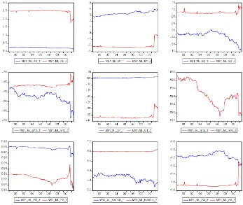
In terms of point parameter estimates, we did not find many differences between the Bayesian and ML estimates, once the label-switching problem of the MS models was properly ac-counted for (for details, see Geweke and Amisano 2004). For this reason, we decided to report only point ML estimates of the parameters in Figures 1–3.
Figure 1 shows the estimation results of the LIN model. Note that individual parameters seem to vary quite a lot, but the es-timated NAIRU (bottom left)NAIRU = −α0/γ1 and the esti-mated “speed of adjustment” (SP, degree of mean reversion, bottom center) sp=β1+β2+β12−1 tend to be more
sta-ble. In particular, the estimated NAIRU is quite high, hovering around 6%, with only a slight drop in the second half of the 1990s. This is in contrast to previous results in the literature
Figure 1. Linear Model (LIN) ML Parameter Estimates.
(e.g., Steiger, Stock, and Watson 2001) documenting that the PC, and the NAIRU in particular, changed radically in the pro-longed expansion that took place in the 1990s. The estimated speed of adjustment, measuring the degree of mean reversion,
can be viewed as indicating how easy it is to forecast changes of inflation in the short term: When SP becomes more negative, as from 1999 onward, it becomes harder to forecastπt, at least in the short term.
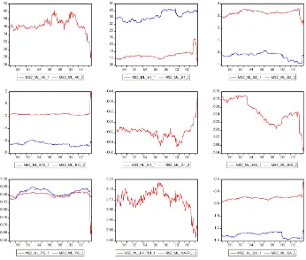
Figure 2. Markov-Switching Model (MS1) ML Parameter Estimates.
Figure 3. Markov-Switching Model (MS2) ML Parameter Estimates.
Figure 2 reports ML parameter estimates of the conditional mean parametersδand the precision parameterh=σ−2for the MS1 model. Note that (1) the MS model parameter estimates are more stable than their LIN model counterpart; (2) the inter-pretation of state 1 being “expansion” and state 2 being “reces-sion” is coherent with the findings that the NAIRU in state 2 is higher than in state 1 and that the persistence of state 1,p11,
is higher than the persistence of state 2, p22 (consistent with
recessions having shorter duration than expansions); and (3) in state 2, NAIRU is almost constant, whereas in state 1 it drops sharply in the second half of the 1990s.
Figure 3 reports results of the estimation of MS2 model. Note that (1) it is problematic to identify states (they have the same persistence, and they are associated with the same
NAIRU; state 1 is associated with higher speed of adjustment); (2) NAIRU estimates are in the same range as for the LIN model, and they have the same time evolution; and (3)h has the same time evolution as in the LIN and MS1 cases.
Turning to the evaluation of the density forecast performance of the competing models, we consider the sequence of one-step-ahead density forecasts implied by the three models, using the ML, FB, and EB estimation approaches. We conduct pairwise WLR tests and report the results in Tables 3A–3C. The main entries are the values ofWLRm,n,the numerator of our test sta-tistic (4), and the numbers within parentheses are thepvalues of the WLR test.
Table 3A reports the unweighted (ω0) case. The table shows
that LIN is significantly worse than either MS1 or MS2. This
Table 3A. Weighted Likelihood Ratio Tests: Unweighted (ω0)
Benchmark LIN–ML LIN–FB LIN–EB MS1–ML MS1–FB MS1–EB MS2–ML MS2–FB
LIN–FB .0004 (.8717)
LIN–EB −.0011 −.0014 (.5671) (.1424)
MS1–ML −.0886∗ −.089∗ −.0875∗
(0) (0) (0)
MS1–FB −.0487∗ −.0491∗ −.0476∗ .0399∗
(0) (0) (0) (0)
MS1–EB .0131 .0128 .0142 .1017∗ .0618∗ (.5095) (.5102) (.4615) (0) (.0008)
MS2–ML −.0478∗ −.0482∗ −.0467∗ .0408∗ .0009 −.061∗ (0) (0) (0) (.001) (.9402) (.0067)
MS2–FB −.0221∗ −.0224∗ −.021∗ .0665∗ .0266∗ −.0352 .0258∗ (0) (0) (0) (0) (.001) (.0627) (.0019)
MS2–EB .0058 .0055 .0069 .0944∗ .0545∗ −.0073 .0536∗ .0279∗ (.6417) (.6647) (.562) (0) (.0002) (.6943) (.0042) (.019)
Table 3B. Weighted Likelihood Ratio Tests: Center (ω1)
Benchmark LIN–ML LIN–FB LIN–EB MS1–ML MS1–FB MS1–EB MS2–ML MS2–FB
LIN–FB −.0002 (.6084)
LIN–B −.0013∗ −.0011∗ (.0017) (0)
MS1–ML −.0338∗ −.0336∗ −.0325∗
(0) (0) (0)
MS1–FB −.0196∗ −.0193∗ −.0182∗ .0143∗
(0) (0) (0) (0)
MS1–EB −.0061 −.0059 −.0048 .0277∗ .0134∗ (.1891) (.1942) (.2918) (0) (.0013)
MS2–ML −.0128∗ −.0126∗ −.0115∗ .021∗ .0067∗ −.0067
(0) (0) (0) (0) (.02) (.1728)
MS2–FB −.0093∗ −.009∗ −.0079∗ .0245∗ .0103∗ −.0032 .0036∗
(0) (0) (0) (0) (0) (.4718) (.0437)
MS2–EB −.0121∗ −.0119∗ −.0107∗ .0217∗ .0075∗ −.006 .0008 −.0028 (0) (0) (0) (0) (.0071) (.1799) (.8254) (.1498)
finding is robust to the estimation method: Using both the ML and the FB approaches, LIN fares significantly worse than both competitors. Using the EB approach, the conclusions are not that clearcut, because the differences are not significant. As for comparison between MS1 and MS2, they are not significantly different for the EB case, but MS1 outperforms MS2 in both the ML and FB estimation cases. In general, we conclude that the winner seems to be the MS1 model and that the best perfor-mance is achieved by using ML estimation.
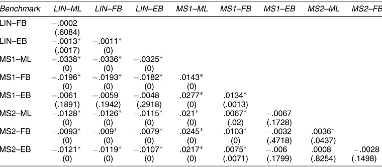
Table 3B shows the results for the center-weighted case (ω1). The conclusions are nearly the same as in the previous case: MS1 dominates MS2 and LIN, both in the classical estimation framework (ML) and in a Bayesian context (FB). Using the EB approach generally yields insignificant differences.
Table 3C reports the results for the tail-weighted case (ω2). Here we have partially different results: In fact, using the ML results, LIN is significantly worse than MS2 only, but the MS1– MS2 difference is not significant. These conclusions are not ro-bust to estimation and forecasting method: FB differences are not significant at all, whereas EB shows dominance of the LIN model. We believe that these findings are due to the fact that the weighting scheme assigns negligible weights to observa-tions near the sample mean of the dependent variable infla-tion, in this way blurring the differences among models. This
interpretation is confirmed by visual inspection of the sam-ple weights (see Fig. 4, bottom center), in which it is evident that nearly half of the observations are assigned weights close to 0.
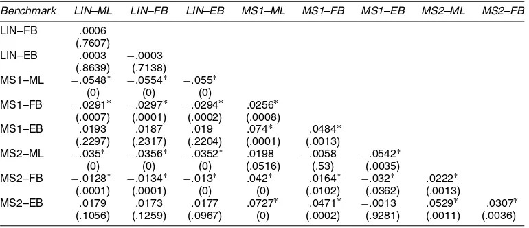
Table 3D shows the results for the right-tail-weighted case (ω3). This weighting scheme can be viewed as assigning
importance to good density forecast properties when inflation is rising fast. The conclusions in this case are very similar to the unweighted case: LIN is significantly outperformed by MS1 and MS2, and this is robust to the estimation method (ML and FB). MS1 outperforms MS2, robust with respect to the estima-tion method (ML, FB). The MS1 appears to be the best model and the best way to obtain density forecasts is to use ML esti-mation.
Table 3E reports the results for the left-tail-weighted case (ω4). In this case, LIN is also significantly worse than MS1 and MS2, with both the ML and FB approaches, and the evidence for EB estimation is not significant. Note also that in this case MS1 is significantly better than MS2 only in the FB approach.
Summing up, it appears that the Markov-switching MS1 model outperforms both alternatives. This happens in the un-weighted case and in most of the un-weighted cases. Only in the tail-weighted (ω2) case do we have a less clear picture, but this
Table 3C. Weighted Likelihood Ratio Tests: Tails (ω2)
Benchmark LIN–ML LIN–FB LIN–EB MS1–ML MS1–FB MS1–EB MS2–ML MS2–FB
LIN–FB .001 (.5612)
LIN–EB .0023 .0013 (.0537) (.1117)
MS1–ML −.0038 −.0047 −.0061 (.678) (.5946) (.4902)
MS1–FB .0003 −.0006 −.002 .0041 (.957) (.9066) (.7157) (.4316)
MS1–EB .0285∗ .0275∗ .0262∗ .0323∗ .0282∗ (.012) (.0124) (.0161) (.0201) (.0098)
MS2–ML −.0156∗ −.0166∗ −.0179∗ −.0118 −.0159∗ −.0441∗ (.0121) (.0072) (.0054) (.118) (.0134) (.0016)
MS2–FB .0012 .0003 −.0011 .005 .0009 −.0273∗ .0168∗ (.6073) (.9226) (.6394) (.4946) (.8389) (.013) (.0014)
MS2–EB .0361∗ .0352∗ .0338∗ .0399∗ .0358∗ .0076 .0517∗ .0349∗ (.0001) (.0003) (.0002) (.0011) (.0006) (.4704) (.0001) (.0001)
Figure 4. Sample Weights Used in DF Comparison Tests.
is likely caused by excessive penalty attributed to the values near the center of the distribution of the dependent variable. We also generally conclude that maximum likelihood estima-tion yields better forecasts than Bayesian estimaestima-tion.
7. CONCLUSION
We introduced a weighted likelihood ratio test for comparing the out-of-sample performance of competing density forecasts of a variable. We proposed measuring the performance of the density forecasts by scoring rules which are loss functions de-fined over the density forecast and the outcome of the variable. In particular, we restricted attention to the logarithmic scoring rule and suggested ranking the forecasts according to the rel-ative magnitude of a weighted average of the scores measured over the available sample. We showed that the use of weights introduces flexibility by allowing the user to isolate the perfor-mance of competing density forecasts in different regions of the unconditional distribution of the variable of interest. Loosely speaking, the test can help distinguish, for example, the rela-tive forecast performance in “normal” days from that in days when the variable takes on “extreme” values. The special case
of equal weights is also of interest, because in this case our test is related to Vuong’s (1989) likelihood ratio test for nonnested hypotheses. Unlike Vuong’s (1989) test, however, our test is performed out of sample rather than in sample, it is valid for both nested and nonnested forecast models, and it considers time series rather than iid data. A further distinguishing feature of our approach is that our null hypothesis is stated in terms of parameter estimates rather than population parameter values, as in Giacomini and White (2006).
Our test can be applied to time series data characterized by heterogeneity and dependence (including possible structural changes), and it is valid under general conditions. In partic-ular, the underlying forecast models can be either nested or nonnested and the forecasts can be produced by using para-metric as well as semiparapara-metric, nonparapara-metric, or Bayesian estimation procedures. The only requirement that we impose is that the forecasts be based on a finite estimation window (see Giacomini and White 2006).
We applied our test to a comparison of density forecasts pro-duced by different versions of a univariate Phillips curve, based on monthly U.S. data over the last 40 years: a linear regres-sion, a two-state Markov-switching regresregres-sion, and a two-state
Table 3D. Weighted Likelihood Ratio Tests: Right Tail (ω3)
Benchmark LIN–ML LIN–FB LIN–EB MS1–ML MS1–FB MS1–EB MS2–ML MS2–FB
LIN–FB −.0002 (.6084)
LIN–EB −.0013∗ −.0011∗ (.0017) (0)
MS1–ML −.0338∗ −.0336∗ −.0325∗
(0) (0) (0)
MS1–FB −.0196∗ −.0193∗ −.0182∗ .0143∗
(0) (0) (0) (0)
MS1–EB −.0061 −.0059 −.0048 .0277∗ .0134∗ (.1891) (.1942) (.2918) (0) (.0013)
MS2–ML −.0128∗ −.0126∗ −.0115∗ .021∗ .0067∗ −.0067
(0) (0) (0) (0) (.02) (.1728)
MS2–FB −.0093∗ −.009∗ −.0079∗ .0245∗ .0103∗ −.0032 .0036∗
(0) (0) (0) (0) (0) (.4718) (.0437)
MS2–EB −.0121∗ −.0119∗ −.0107∗ .0217∗ .0075∗ −.006 .0008 −.0028 (0) (0) (0) (0) (.0071) (.1799) (.8254) (.1498)
Table 3E. Weighted Likelihood Ratio Tests: Left Tail (ω4)
Benchmark LIN–ML LIN–FB LIN–EB MS1–ML MS1–FB MS1–EB MS2–ML MS2–FB
LIN–FB .0006 (.2297) (.2317) (.2204) (.0001) (.0013)
MS2–ML −.035∗ −.0356∗ −.0352∗ .0198 −.0058 −.0542∗ (0) (0) (0) (.0516) (.53) (.0035)
MS2–FB −.0128∗ −.0134∗ −.013∗ .042∗ .0164∗ −.032∗ .0222∗ (.0001) (.0001) (0) (0) (.0102) (.0362) (.0013)
MS2–EB .0179 .0173 .0177 .0727∗ .0471∗ −.0013 .0529∗ .0307∗ (.1056) (.1259) (.0967) (0) (.0002) (.9281) (.0011) (.0036)
Markov-switching regression in which the natural rate of unem-ployment was constrained to be equal across states. Note that these models imply different shapes for the density of inflation: a normal density for the linear model and a mixture of normals for the Markov-switching models. In the comparison, we also considered versions of each model estimated by maximum like-lihood or by Bayesian techniques.
Our general conclusion was that density forecasts from the two-state Markov-switching model outperformed all alterna-tives. This happened in the unweighted case and in most of the weighted cases. Only in the tail-weighted case could the three models not be discriminated, but this is likely caused by exces-sive penalization of the values near the center of the distribu-tion of the dependent variable. We also found that maximum likelihood estimation yielded superior forecasts than Bayesian alternatives.
ACKNOWLEDGMENTS
We are deeply indebted to Clive W. J. Granger for many inter-esting discussions. We also thank the editor, the associate editor, and two anonymous referees for constructive suggestions, and Carlos Capistran, Roberto Casarin, Graham Elliott, Ivana Ko-munjer, Andrew Patton, Kevin Sheppard, Allan Timmermann, and seminar participants at the University of Brescia for valu-able comments. This article was previously circulated under the title “Comparing Density Forecasts via Weighted Likelihood Ratio Tests: Asymptotic and Bootstrap Methods” by Raffaella Giacomini.
APPENDIX A: HYPERPARAMETERS
With reference to (19) and (20), in the LIN model we used as hyperparameters
For the MS1 and MS2 models, we used the same hyperpara-meters,s=.3,ν=3, as in the LIN model; for the regression coefficients, we used the following prior hyperparameters:
MS1: µ
whereas for the Dirichlet prior for the rows ofP, we used
R=
We show that assumptions (i)–(iii) of theorem 6 of Giacomini and White (2006) (which we denote by GW1–GW3) are satis-fied by lettingWt≡Zt andLm,t+1≡WLRm,t+1, from which
(a) and (b) follow.
GW1 coincides with assumption 1.
GW2 imposes the existence of 2rmoments ofWLRm,t+1=
w(Yt+1)(logfˆm,t(Yt+1)−loggˆm,t(Yt+1))for somer>2. From
assumption 2, there exists anr′>2 such that
E|logfˆm,t(Yt+1)|2r
≤Ew(Ytst+1)2r(1+ε)/εε/(1+ε)E|logfˆm,t(Yt+1)|2r(1+ε)
1/1+ε
=Ew(Ytst+1)2r′/εε/(1+ε)E|logfˆm,t(Yt+1)|2r
′1/(1+ε)
<∞,
where the last inequality holds because the first term is fi-nite becausew(·)is bounded, and the second term is finite by assumption 2. Similarly,E|w(Ytst+1)loggˆm,t(Yt+1)|2r<∞. By Minkowski’s inequality, we, thus, have
E|WLRm,t+1|2r
Finally, GW3 coincides with assumption 3.
Proof of Proposition 2
[Received July 2002. Revised March 2006.]
REFERENCES
Andrews, D. W. K. (1991), “Heteroskedasticity and Autocorrelation Consistent Covariance Matrix Estimation,”Econometrica, 59, 817–858.
Artzner, P., Delbaen, F., Eber, J. M., and Heath, D. (1997), “Thinking Coher-ently,”Risk, 10, 68–71.
Bai, J. (2003), “Testing Parametric Conditional Distributions of Dynamic Mod-els,”Review of Economics and Statistics, 85, 531–549.
Berkowitz, J. (2001), “The Accuracy of Density Forecasts in Risk Manage-ment,”Journal of Business & Economic Statistics, 19, 465–474.
Bolleslev, T., Engle, R., and Nelson, D. (1994), “ARCH Models,” inHandbook of Econometrics, Vol. IV, eds. R. F. Engle and D. McFadden, Amsterdam: Elsevier.
Christoffersen, P. F., and Diebold, F. X. (1997), “Optimal Prediction Under Asymmetric Loss,”Econometric Theory, 13, 808–817.
Clements, M. P., and Hendry, D. F. (1999),Forecasting Non-Stationary Eco-nomic Time Series, Cambridge, MA: MIT Press.
Clements, M. P., and Smith, J. (2000), “Evaluating the Forecast Densities of Linear and Nonlinear Models: Applications to Output Growth and Unem-ployment,”Journal of Forecasting, 19, 255–276.
Corradi, V., and Swanson, N. (2005), “A Test for Comparing Multiple Misspec-ified Conditional Distributions,”Econometric Theory, 21, 991–1016.
(2006a), “Bootstrap Conditional Distribution Tests in the Presence of Dynamic Misspecification,”Journal of Econometrics, in press.
(2006b), “Predictive Density and Conditional Confidence Interval Ac-curacy Tests,”Journal of Econometrics, in press.
Diebold, F. X., Gunther, T. A., and Tay, A. S. (1998), “Evaluating Density Fore-casts With Applications to Financial Risk Management,”International Eco-nomic Review, 39, 863–883.
Diebold, F. X., and Lopez, J. A. (1996), “Forecast Evaluation and Combina-tion,” inHandbook of Statistics: Statistical Methods in Finance, Vol. 14, eds. G. S. Maddala and C. R. Rao, Amsterdam: North-Holland, pp. 241–268. Diebold, F. X., and Mariano, R. S. (1995), “Comparing Predictive Accuracy,”
Journal of Business & Economics Statistics, 13, 253–263.
Diebold, F. X., Tay, A. S., and Wallis, K. F. (1999), “Evaluating Density Fore-casts of Inflation: The Survey of Professional Forecasters,” inFestschrift in Honour of C. W. J. Granger, eds. R. Engle and H. White, Oxford, U.K.: Ox-ford University Press, pp. 76–90.
Duffie, D., and Pan, J. (1996), “An Overview of Value at Risk,”Journal of Derivatives, 4, 13–32.
Geweke, J., and Amisano, G. (2004), “Compound Markov Mixture Models With Applications in Finance,” working paper, University of Brescia. Giacomini, R., and White, H. (2006), “Tests of Conditional Predictive Ability,”
Econometrica, in press.
Hansen, B. E. (1994), “Autoregressive Conditional Density Estimation,” Inter-national Economic Review, 35, 705–730.
Hong, Y. (2000), “Evaluation of Out-of-Sample Density Forecasts With Appli-cations to S&P 500 Stock Prices,” unpublished manuscript, Cornell Univer-sity.
Hong, Y., and Li, H. (2005), “Nonparametric Specification Testig for Continuous-Time Models With Applications to Term Structure of Interest Rate,”Review of Financial Studies, 18, 37–84.
Hong, Y., and White, H. (2005), “Asymptotic Distribution Theory for Non-parametric Entropy Measures of Serial Dependence,” Econometrica, 73, 837–901.
Kim, C. J., and Nelson, C. (1999),State Space Models With Regime Switching, Cambridge, MA: MIT Press.
Lopez, J. A. (2001), “Evaluating the Predictive Accuracy of Volatility Models,”
Journal of Forecasting, 20, 87–109.
Newey, W. K., and West, K. D. (1987), “A Simple, Positive Semidefinite, Het-eroskedasticity and Autocorrelation Consistent Covariance Matrix,” Econo-metrica, 55, 703–708.
Patton, A. J. (2006), “Modelling Asymmetric Exchange Rate Dependence,” In-ternational Economic Review, 47, 527–556.
Sims, C. A., and Zha, T. (2006), “Were There Regime Switches in U.S. Mone-tary Policy?”American Economic Review, in press.
Soderlind, P., and Svensson, L. (1997), “New Techniques to Extract Market Expectations From Financial Instruments,”Journal of Monetary Economics,
40, 383–429.
Steiger, D., Stock, J. H., and Watson, M. W. (2001): “Prices, Wages and the U.S. NAIRU in the 1990s,” Working Paper 8320, National Bureau of Economic Research.
Stock, J. H., and Watson, M. W. (1999), “Forecasting Inflation,”Journal of Monetary Economics, 44, 293–335.
Tay, A. S., and Wallis, K. F. (2000), “Density Forecasting: A Survey,”Journal of Forecasting, 19, 235–254.
Vuong, Q. H. (1989), “Likelihood Ratio Tests for Model Selection and Non-Nested Hypotheses,”Econometrica, 57, 307–333.
Weigend, A. S., and Shi, S. (2000), “Predicting Daily Probability Distributions of S&P 500 Returns,”Journal of Forecasting, 19, 375–392.
Weiss, A. A. (1996), “Estimating Time Series Models Using the Relevant Cost Function,”Journal of Applied Econometrics, 11, 539–560.
West, K. D. (1996), “Asymptotic Inference About Predictive Ability,” Econo-metrica, 64, 1067–1084.
Winkler, R. L. (1967), “The Quantification of Judgement: Some Method-ological Suggestions,”Journal of the American Statistical Association, 62, 1105–1120.