202
9
the Financing of a Firm
C O N C E P T S
● Explicit Costs ● Implicit Costs
● Accounting Costs ● Economic Costs
● Short-run Cost Concepts ● Long-run Cost Concepts
● Fixed or Total Fixed Cost ● Overhead Costs
● Variable Cost or Total Variable Cost ● Total Cost
● Marginal Cost ● Average Fixed Cost
● Average Variable Cost ● Average Cost or Average Total Cost
● Plant Size ● Economies of Scale
● Division of Labour ● Diseconomies of Scale
● Social Cost ● Private Cost
● Externality ● Positive Externality
● Negative Externality ● Plough Back of Profits
● Retained Earnings ● Loans from Financial Institutions
T
owards the end of the last chapter we saw that as output increases, the total cost rises. But there is much more to it than just that. In this chapter we study in detail various types of costs and their relation to output.To begin with, there are explicit costs and implicit costs. Explicit costsare those, which are directly paid to other parties by an entrepreneur or a company running a business. They include, for example, the costs of labour, raw material, machinery purchased and so on. Implicit costsare those for which there is no direct payment but indirectly there is a cost involved.
Suppose you own a two-storey building. You live on the first floor and operate a small publishing company on the ground floor. Obviously, you do not have any rental cost of business operation. But there is an implicit cost. If you had otherwise rented out the ground floor to some other party, you would have obtained some rental income. By using it for your own business, you are effectively losing that income—and that is an implicit cost. Similarly, if you use your own savings in the business, the interest income foregone is an implicit cost.
Explicit costs are more commonly called accounting costs. Accounting costs plus implicit costs of the kind described above reflect the true cost of running a business and are called economic costs. In economic analysis, costs always refer to economic costs.
In this chapter, we will be concerned with various cost concepts based on the time horizon of an entrepreneur, namely, the short run and the long run. There is no par-ticular calendar time like a month, quarter or year that distinguishes between the short run and the long run. Rather, as will be seen, the distinction is drawn from a production planning perspective.
SHORT-RUN COST CONCEPTS
If you think of a firm at a given point of time, like a snapshot, everything is fixed. The firm is producing a given amount by using a given amount of inputs and the inputs are paid their prices. All costs are given or fixed. But if we imagine the func-tioning of a firm over a relatively short length of time (like a movie), we can distin-guish between costs that are fixed and those that are not. Suppose you run a clothing store. In a span of, say, one or two months, it is likely that the rental cost of the rooms you use are fixed in the sense that how much you pay as rent does not depend on how much you sell or produce. You may have signed a lease with the landlord for six months with a specified rent and your landlord (unless he is very kind) is going to charge you that rent—irrespective of how well you are doing in your business or even if you decide to produce nothing. That is why, generally, the rental cost is con-sidered fixed in the short run. But typically labour costs are not fixed because work-ers can be hired and fired on a short notice by a firm. Costs of raw materials (for example, cloth bought in the wholesale market) are not fixed as you can buy more or less of them depending on the state of your business.
nurses, technicians, management employees and manual workers. By taking loans from a bank he has bought several high-tech machines that do CAT scan, MRI, ultrasound tests and so on. Every month he repays the bank Rs 2 lakh in instalment towards his loan plus interest. This is an example of fixed cost because it is inde-pendent of how many patients come to Dr Juneja’s centre for service. There is also an implicit rental cost of the flat, equal to the rent foregone by using the flat for the diagnostic centre. This is also a fixed cost. However, depending on how this ven-ture is going, Dr Juneja can hire more or less of nurses or manual workers within a short notice. Hence, payment to nurses and other workers are not fixed.
Over a longer time horizon, however, an entrepreneur can think of explicitly or implicitly renting a different amount of space, a different plant size, different number of machines and so on. In other words, in the long run there are no fixed costs.
Returning to the short run, we then say that a firm has two types of costs, fixed costand variable cost. Fixed costs are those costs that do not change with output. In common business terminology, these are called overhead costs. Variable costs refer to those that vary with the output. Typically, rental costs of land and capital are fixed and labour and raw material costs are variable.
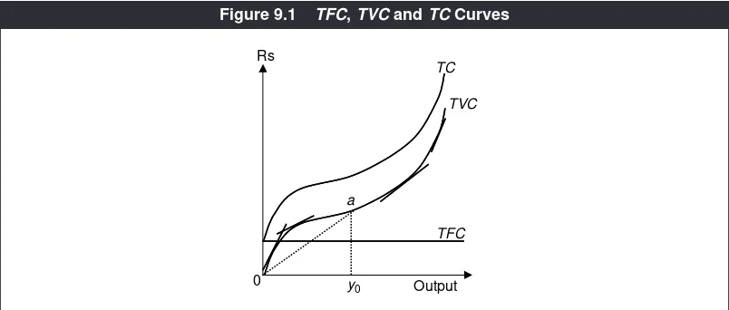
More formally, these are respectively called total fixed cost (TFC) and total variable cost(TVC). The sum of the two costs is simply called the total cost(TC). That is,
TC=TFC+TVC. (9.1)
These costs—TFC, TVCand TC—when graphed against the output, give us the TFC, TVC and TC curves respectively. See Figure 9.1 (but ignore for now the tangents, the point aand the dotted lines from this point). The TFC curve is a horizontal straight line (having zero slope) because TFCis independent of the output level. The TVCcurve is upward sloping because producing more would cost more.
TVC
0 Rs
TC
TFC
Output a
y0
Since TCis the sum of TFCand TVCand costs are measured along the vertical axis, the TCcurve is the vertical sum of the TFCand TVCcurves. That is, at any output level, if we measure the TFCand TVCon the vertical axis and add them up, we get the corresponding point on the TCcurve.
Like the marginal product and average product, we define marginal cost and average cost. Marginal cost(MC) is the addition to the total variable cost per one extra unit produced. It is also equal to the addition to the total cost per one extra unit produced since the difference between the TVCand TCis fixed. In the graph,
MCis the slope of the TVCand the TCcurves. You see in Figure 9.1 that as the out-put increases, the slope of TVCinitially falls and then rises. This means that the
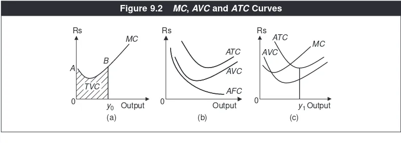
MC curve (measuring MC against output) will be downward sloping first and then upward sloping. Put differently, it is U-shaped as shown in Figure 9.2(a). Also, since MCis the addition to the TVC, the area under the MCcurve equals theTVC.1
Similarly, we can define
Average Fixed Cost (AFC) ≡ TFC/Output
Average Variable Cost (AVC) ≡ TVC/Output
Average Total Cost (ATC) ≡ TC/Output,
where the symbol ‘≡’ means ‘equal to by definition’. The AFC, AVC and ATC
curves are drawn in Figure 9.2(b). The AFCis uniformly downward sloping by its definition—as output increases, its denominator increases while the numerator remains unchanged.2The shapes of the AVCand ATCcurves depend on the shape
of the TVCor the TCcurve. Referring back to Figure 9.1 again, see that at output y0, for instance, TVC= y0aand thus AVC= y0a/0y0, which is the slope of the ray 0a. If we let the output gradually increase from zero, this slope increases up to a point and then decreases. This implies that the AVCcurve will be U-shaped. The argu-ment behind the ATCcurve being U-shaped is similar.
0
Figure 9.2 MC, AVC and ATC Curves
1It cannot be equal to TC as it cannot account for the fixed cost.
2Indeed, the AFC curve is shaped like, what is called in geometry, a rectangular parabola, analogous to the unitarily elastic
Finally, turn to Figure 9.2(c) (and ignore for now the output marked y1). The mathematical relationship between the ‘average’ (A) and the ‘marginal’ (M) holds. Remember from the last chapter that M< Aif Ais falling and M> Aif Ais rising. Since AVCfalls initially, MC< AVC; when AVCrises, MC> AVC.The implication is that the MCcurve must cut the AVCcurve at the latter’s minimum point. The same relationship holds between the MCcurve and the ATCcurve.
NUMERICAL EXAMPLE 9.1
A firm’s total cost of producing 4 units of output is Rs 70. Its marginal cost sched-ule is given in Table 9.1. What is the firm’s total fixed cost? Derive the firm’s
TCschedule and TVCschedule.
The marginal cost of producing 4 units is Rs 6, which is the additional cost of pro-ducing the fourth unit. Since the total cost of propro-ducing 4 units is Rs 70, the total cost of producing 3 units must be Rs 70 – Rs 6 = Rs 64. Extending the same logic, the total costs of producing 2 units, 1 unit and 0 units are respectively equal to Rs 59, Rs 52 and Rs 42. The total variable cost of producing 0 units is 0 by definition. Hence Rs 42 being the total cost of producing 0 implies that it is equal to the total fixed cost. Using the relationship between the marginal cost and the total cost, and the mar-ginal cost information for outputs 5, 6 and 7 units given in Table 9.1, we obtain the total cost at these output levels equal to Rs 78, Rs 89 and Rs 103. We now have
Table 9.2 TC and TVC Schedules (Numerical Example 9.1)
Output TC TVC
0 42 0
1 52 10
2 59 17
3 64 22
4 70 28
5 78 36
6 89 47
7 103 61
Table 9.1 MC Schedule (Numerical Example 9.1)
Output Total Cost (Rs)
0 –
1 10
2 7
3 5
4 6
5 8
6 11
the entire total cost schedule. Deducing Rs 42 (the TFC) from it, we obtain the TVCschedule. These schedules are given in Table 9.2.
Why are
MC
,
AVC
and
ATC
Curves U-shaped?
The U-shape of the MC, AVCand ATC curves followed from the TC and TVC curves drawn in Figure 9.1. But this is not the basic economic reason behind why the MC, AVCand ATCcurves are U-shaped—we could have drawn these curves first and then obtained the TCand the TVCcurves from these. The underlying rea-son is the law of diminishing returns, studied in the last chapter.
Recall that this law states that initially the MPPof a factor may be increasing but after a certain point it must start to diminish. This means that if some other inputs are kept unchanged—there are fixed factors and hence there are fixed costs in the short run—initially when a factor’s MPPis increasing, a gradual increase in output by a given amount would require a decrease in the rate of increase of the variable inputs and, therefore, a decrease in the rate of increase of the total cost of variable inputs. But the rate of increase of the total cost of variable inputs is equal to MC by definition. Thus, initially, MC decreases with output. After a certain point when diminishing returns set in, a gradual increase in output by a given amount would require an increase in the rate of increase of the total cost of vari-able inputs. This translates into MC increasing with output. In summary then, MCinitially decreases with output and then increases with it after a certain point. That is, the MCcurve is U-shaped.3The U-shape of the MCcurve implies that the AVCand ATCcurves are also U-shaped and that is why TCand TVCcurves look like the way they do in Figure 9.1.4
Shift of the Short-run Cost Curves
What are the factors that shift the short-run cost curves? These are technology, input prices, the level of fixed factors and business taxes. A technology improve-ment enables more output being generated from the same levels of inputs. It would lower costs and, in general, shift down TC, TVC, AVC, ATCand MCcurves. An increase in the price of fixed factors would shift up the TFC, AFC, ATC and TCcurves, while TVC, AVCand MCcurves will remain unchanged. An increase in the price of variable factors would not shift TFCand AFC curves but would shift the other curves up.
The positions of the short-run variable and marginal cost curves depend crucially on the levels of fixed inputs. Since fixed inputs typically are heavy machinery, land and so on, the levels of fixed inputs define what is briefly called the plant size. Hence we can say that the plant size determines the positions of TVC, AVCand MC curves. In particular, the output at which the ATC attains its minimum can be
3In other words, the MC curve is the mirror image of the MPP curve.
interpreted as the most efficient output level corresponding to the plant size. For instance, if you go back to Figure 9.2(c), the most efficient output level relative to the underlying plant size is y1. An output higher or less than y1means over-utilising or under-utilising the plant so that the unit cost is greater than the minimum ATC.
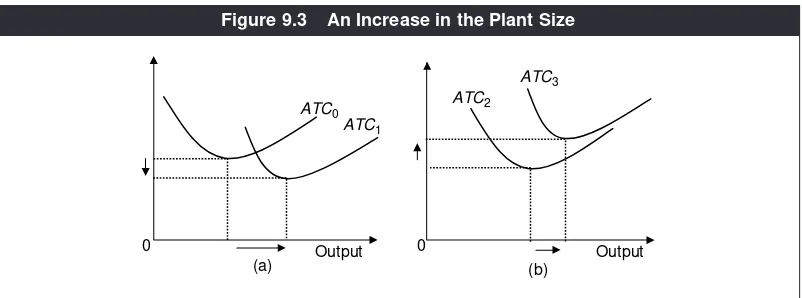
Now consider an increase in the plant size. With a bigger plant, the most effi-cient level of output will be higher. This is illustrated in both panels of Figure 9.3. However, will it mean a lower minimum ATCor a higher minimum ATC? That depends on the initial plant size. If it is relatively small, an increase in plant size would reduce the minimum ATC because of increasing returns to scale (to be discussed later). Otherwise, if the initial plant size is sufficiently large, a fur-ther increase in the plant size will raise the minimum ATCbecause of decreasing return to scale (to be discussed later). These possibilities are shown respectively in panels (a) and (b) of Figure 9.3.
As discussed in Chapter 3, businesses pay various taxes to the government like excise tax and VAT, because of their production activities. Such tax payments add to the direct production costs of firms. Thus an increase in the rate of business taxes will shift up the short-run ATC, AVCand MCcurves.
LONG-RUN COST CONCEPTS
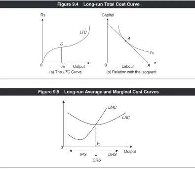
In the long run, a producer has more options compared to the short run. Contracts can be changed. Plant sizes can be increased or decreased. In fact, the quantity of any input can be varied. There are no fixed costs. All costs are variable. Thus we simply say ‘total cost’ instead of ‘total variable cost.’ The TCcurve shapes up like the TVC curve, passing through the origin. This is shown in Figure 9.4(a) and marked as the LTCcurve (‘L’ standing for ‘long run’ ).
We can link the long-run total cost with the isoquant analysis in the previous chapter. Each point on the long-run TCcurve is the minimum cost associated with the corresponding isoquant. (The same holds for the total variable cost in the short run.) Consider, for instance, an output level of y0. Panel (b) of Figure 9.4 shows its
Output
(a) (b)
0
ATC3
ATC0 ATC2
ATC1
0 Output
isoquant. Cost minimisation occurs with the input bundle A. The total cost of this bundle, in terms of say labour, is B. In terms of money this is equal to 0B×wage
rate, which in turn equals the total cost y0Cin panel (a).
However, the concept of marginal cost remains the same. We call it the long-run marginal cost or LMC. There is no difference between AVCand ATC. Instead, we call it the long-run average cost or LAC.
In general, both LMCand LACcurves are U-shaped, similar to the short-run marginal and average cost curves, as shown in Figure 9.5. But the underlying rea-son is different and not the law of diminishing returns. This does not mean that for any factor, this law only holds in the short run but not the long run. The dif-ference, however, is that since all factors are variable, it is the nature of returns to scale (studied in the last chapter) which determines how the long-run costs may change with output. For instance, if there are increasing returns to scale (IRS), a proportionate change in all inputs leads to a more than proportionate change in the output. This means, for example, that a 10 per cent increase in output can be
A
Capital
0
C
Rs
Output Labour B
0
(a) The LTC Curve (b) Relation with the Isoquant
y0
y0 LTC
Figure 9.4 Long-run Total Cost Curve
LAC LMC
Output
IRS DRS
CRS y0 0
obtained by a 7 per cent increase in all inputs. In terms of costs, it means that a 10 per cent increase in output will lead to a 7 per cent increase in the total cost and, thus, implies a decline in the average cost. Hence,
IRS⇒ LAC falls with output.
Similar reasoning implies:
Decreasing Returns to Scale (DRS)⇒LAC rises with output
Constant Returns to Scale (CRS)⇒ LAC is constant.
Therefore, a U-shaped LAC curve, as shown in Figure 9.5, which means that LAC first declines, then remains constant (at the minimum point) and finally increases, is built on the assumption that as a firm contemplates higher and higher output in the long run, it experiences IRSfirst, CRSnext and DRSfinally. The eco-nomic rationale behind this sequence is as follows.
Starting from a small scale of output or plant size, an expansion enables a firm to implement further division of labour. That is, the firm will be able to allocate its workers to the specialised jobs they are best at. For instance, if initially a firm has one secretary who does typing as well as answers customers, then, as business improves and the firm is in a position to hire, say, two secretaries, it can hire one who is really good at typing and another who is good at dealing with the public. Compared to the initial situation, twice the amount of original work is done now and that too more efficiently. Division of labour tends to reduce the long-run aver-age cost. Another benefit from expansion of output could come from volume dis-counts in buying inputs. Higher output requires more inputs and in purchasing inputs in bulk, a producer may get discounts. This would also tend to lower the average cost. These are the reasons why the long-run average cost may fall with an increase in output. In other words, these are the sources of increasing returns to scale—also called economies of scale.
However, after a certain point when the output reaches a critical limit, ineffi-ciency in management creeps in due to overcrowding and congestion of inputs. These are diseconomies of scale, leading to decreasing returns to scale. Any further expansion of output leads to an increase in the plant size accompanied by an increase in the long-run average cost.
In between IRS and DRS, there are neither economies nor diseconomies of scale; instead, the firm experiences CRS. If this happens over an interval of output, the LACwill have a flat segment. Otherwise, it will be just a point.
Our reasoning of why the LACcurve is U-shaped is complete. It is the U-shape of the LACcurve that explains the same shape of the LMCcurve.5
A change in technology, a change in an input price or a change in the rate of business taxes shifts the long-run average and marginal cost curves too. As one would expect, a technology improvement shifts them downward, while an increase in an input price or business taxes shifts them upward.
5This is in contrast to the short run, where the shape of the marginal cost curve determines the shape of the average variable
RELATIONSHIPS BETWEEN SHORT-RUN AND LONG-RUN COST
CURVES
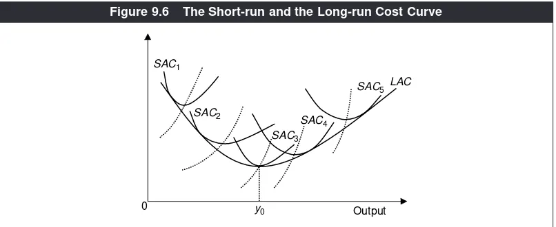
The plant size is given in the short run whereas it can be varied in the long run (by definition). Hence, the long-run cost at any given level of output should take into account the firm’s choice of the plant size. Figure 9.6 depicts a family of short-run AC
and MCcurves. As discussed earlier, a larger plant size is associated with a higher level of the most efficient output. But the minimum ACdecreases or increases with plant size as the initial plant size is relatively small or large. Figure 9.6 exhibits this pattern.
Two points are significant in this regard. (a) The long-run AC cannot be independent of the short-run AC.(b) At any given level of output, the long-run AC
cannot exceed the short-run AC, because there is more flexibility in the long run. Put differently, the firm always has the choice, in the long run, to select the plant size chosen in the short run and hence the LAC cannot be higher. (a) and (b) imply that the LACcurve must be tangential to or an envelop of the family of short-run ACs.
Notice the output level y0at which the LACas well as the associated short-run
AC (SAC) is minimised. At any output level below (or above) y0, the tangency point lies to the left (or right) of the minimum point on the corresponding SAC.
SOCIAL AND PRIVATE COSTS OF PRODUCTION
The cost curves we have studied so far relate to firms or an industry. Do they also reflect the society’s cost of producing the same good? Of course, the firm or the industry in question is a part of the society and thus its costs must be included in the society’s cost. But the industry’s and the society’s cost may not be the same
SAC5
0 SAC1
SAC2 SAC
4
LAC
SAC3
Output y0
always because productive activity by one firm or industry may affect other firms, other industries or households.
Typically, the production of many industrial goods generates industrial waste, causing pollution. Many steel plants emit smoke, which has a very high carbon dioxide content. Wastes from chemical plants are highly polluting. Suppose a chemical plant does not have a proper disposal system and it simply channels its waste to a nearby river.6Many people (and animals) use the river water for a
vari-ety of purposes. Obviously, the polluted water causes health problems—it is an environmental concern.
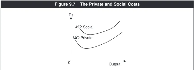
Are the chemical plant’s marginal and average costs same as the society’s mar-ginal and average costs? The answer is no. The plant’s own costs of producing output in terms of payments to labour, raw material, capital, land and so on are its private costs. But they do not include the environmental costs of the output to society at large. The social costs, which must include the cost to the environment, are higher.
In this example, we say that an increase in the firms’ output causes an externality
to society and it is a negative externalityin that the firm’s output, via creating or increasing pollution, adversely affects society.
We term the firm’s own cost as private cost; social costis defined as the sum of the private cost and the cost of the externality caused to society. Figure 9.7 illus-trates these curves in terms of the marginal cost when a negative externality is present.
In some cases there may be a positive externality. Suppose a new nursery has come up close to your neighbourhood. You, as part of the general public, enjoy the smell of flowers and the greenery from plants and small trees. This is an example of positive externality—in this case, the social marginal cost will be less than the private marginal cost.
6In reality, many chemical plants do have proper disposal systems.
Rs
Output
MC: Social
0
MC: Private
HOW DO FIRMS FINANCE THEIR COSTS?
Several concepts regarding costs have been discussed. But you may ask a basic but relevant question that we have not touched upon as yet. That is, how does a firm finance its costs? Put differently, what are the sources of funds from which a firm is able to pay the factors of production?
In general, there are four sources. One is the plough back of profitor what is
called retained earnings, referring to a part of its own accumulated profit being used towards covering some costs. It simply means using the firm’s own money. A small entrepreneur may use part of his profit income for own consumption and invest the rest in his firm. A corporation pays out a part of its profit earnings to shareholders, who are the owners of the firm. The rest are retained earnings, which are ‘ploughed back’ to the firm.
Businesses however, do not always, use their own money for covering costs.
Loans from financial institutionsare another source. A loan is a financial contract
between the lender (the financial institution like a commercial bank) and the bor-rower (the firm), specifying the duration of loan and an interest rate. The lending institution typically reviews the project for which the loan is being requested. Further, as a security to itself, it holds some property of the firm (borrower) as the mortgage. If, for some reason, the firm is not able to pay back the loan, the lend-ing institution has the right to sell off the mortgaged property and use the pro-ceeds to recover its loan. If the sale of the mortgaged property does not fully recover the loan, the firm owners are personally liable to pay the rest.
New stocks and bonds are the remaining two ways of financing. Through issu-ing these, the firm raises funds from the general public. These are already described in Chapter 7. Basically, stocks offer an ownership of the firm whereas bonds do not. Stocks and bonds are respectively equity and debt instruments issued by a firm.
There are trade-offs between these alternative ways of raising funds. It is not in the interest of the company’s management to always plough back a large fraction of profits because this would mean less dividend payments and a smaller return to stockholders. Hence, the public would not want to invest much in the company via buying its stocks. It will be harder for the company to raise money in the future through issuing stocks. On the other hand, it is not wise to always pay back most of the profit earnings to the shareholders because, all else the same, this would leave less amount for plough back and expansion of the company’s operation. A balance has to be struck between dividend payments and retained earnings.
It is also interesting that from the viewpoint of a firm’s management, plough back is the easiest choice because there is no outside scrutiny. If, instead, a com-pany has to issue new bonds or stocks, or even apply for loans to a bank, it has to do a lot of paper work; submit it to the right authorities; and then the company’s performance is evaluated. There is no such thing as perfect management. Hence, some weaknesses are bound to come out in the open. Yet, as we have just dis-cussed, the easiest choice of plough back has its own limitations.
Economic Facts and Insights
● In economic analysis, costs always refer to economic costs—the sum of
explicit (accounting) costs and implicit costs.
● Fixed costs are independent of the output, while variable costs are not. ● The total variable cost in the short run or the total cost in the long run is the
minimised total cost in the cost minimisation problem.
● The short-run average variable and average total cost curves are U-shaped
because the short-run marginal cost curve is U-shaped. The explanation of the latter lies in the law of diminishing returns.
● A technological improvement shifts the cost curves downward, while input
price increases or increases in business taxes shift them upward.
● An increase in the plant size may increase or decrease the minimum
aver-age total cost when there are increasing or decreasing returns to scale respectively.
● The concepts of marginal product and the law of diminishing returns are
valid even in the long run when all factors are variable.
● In the long run, all costs are variable.
● The long-run average cost is U-shaped because, as output expands, a firm
typically experiences increasing returns to scale, followed by constant and decreasing returns to scale. The U-shape of the long-run average cost curve implies the U-shape of the long-run marginal cost curve.
● Division of labour and volume discounts on purchase of inputs are sources
of economies of scale, whereas management inefficiency due to the large scale of operations, overcrowding and congestion of inputs cause diseco-nomies of scale.
● Negative (positive) externalities imply that social marginal cost is higher
(less) than the private marginal cost.
● Pollution imposes a negative externality on society.
● Firms finance their costs through retained earnings, loans from financial
institutions and through issuing new bonds and stocks.
E
E X
X E
E R
R C
C II S
S E
E S
S
9.1 Give a hypothetical—yet related to the real world—example of an implicit cost.
9.2 ‘Economic cost is a part of accounting costs’. Defend or refute. 9.3 What is an overhead cost? Give two examples.
9.4 ‘Marginal cost is the addition to the total cost, not to the total variable cost, per one extra unit produced’. Defend or refute.
9.5 What is the area under the marginal cost curve equal to—total cost or total variable cost?
9.6 Explain why the MC, AVCand ATCcurves are U-shaped?
9.7 Briefly state and explain the relationship between MC, AVCand ATCcurves.
9.8 AVCis minimised at a level of output, which is _____ than that at which ATC
attains its minimum value. Fill in the blank and give reasons.
9.9 What is the vertical difference between the TCand TVCequal to and why?
9.10 A firm’s total cost schedule in the short run is the following. What is its total fixed cost? Derive the marginal cost schedule.
9.11 Briefly describe the relationship between the short-run average cost curve and the long-run average cost curve.
9.12 How does an increase in business taxes shift the marginal and average cost curves?
9.13 How does a technical progress shift the marginal and average cost curves? 9.14 How would an increase in input prices affect the marginal and average cost
curves?
Output Total Cost (Rs)
0 10
1 25
2 35
3 43
4 54
5 69
6 91
7 121
8 161
● As a means of financing its costs or operation, issuing bonds are cheaper but
riskier than issuing stocks for a firm.
● Issuing new bonds and stocks or applying for sizeable loans from financial