Vol. 8 No. 1, p 1 – 20 [email protected] ISSN: 1412-0070
Efisiensi Bank Pembangunan Daerah Menggunakan Data Envelopment
Analysis dan Stochastik Frontier Analysis
Marthen Sengkey*
Fakultas Ekonomi Universitas Klabat
The study employs the three-stage banking models to investigate the performance of 26 state banks in Indonesia from 1994 to 2004. Data envelopment analysis (DEA) results indicate that the average efficiency of state banks was 38.3 percent and deteriorated when the financial crisis struck Indonesia in 1997. Using stochastic frontier analysis (SFA) method, findings suggest that, on average, banks obtained 62.8 percent efficiency. Findings also suggest that banks’ technical inefficiency is affected significantly by government intervention, location, and ownership. Finally, state banking performance was tested by correlating the DEA and SFA models and found no statistically significant correlation. Reported new findings of this paper are additions to banking efficiency literature.
Key words: DEA, state banks, Indonesia, performance, SFA
INTRODUCTION
This study used organization theories to develop such a framework and used that framework to examining the efficiency performance of regional development banks in Indonesia during 1994 through 2004. This theoretical framework was based on theories of state banking, bank management, financial performance (bank balance sheet; financial ratio analysis; capital adequacy), and productive-efficiency theory and inefficiency.
State Banking Theory. Banks are among the most important financial institutions in the economy. They are the principal source of credit (loanable funds) for millions of households (individuals and families) and for most local units of government (school districts, cities, counties, etc) (Rose, 1996). Futher, Rose (1996) states that banks are financial-service firms, producing and selling professional management of the public’s funds as well as performing many other roles in the economy.
During the 1970, Indonesia’s state banks benefited from supportive government policies, such as the requirement that the growing state enterprise sector banks solely with state banks. State banks were viewed as agents of development rather than profitable enterprises, and most state bank lending was in fulfillment of government mandated and subsidized programs designed to promote various economic activities, including state enterprises, and small-scale pribumi businesses. State bank lending was subsidized through Bank Indonesia, which extended “liquidity credits” at very low interest rates to finance various programs. Total state bank lending in turn repressented about 75 percent of all commercial bank lending (U.S. Library of Congress).
*corresponding author
Government banks are sometimes appallingly inefficient; in the absense of competitions, private banks may be just as bad. Further, increasing competition can lead to financial instability, crisis, and public bailout. In contrast, banking regulations in some countries are rigorously enforced; financial policy can nurture internationally competitive industries; and some governments own banks that are profitable and prudent.
State banks will need to undergo sweepong reforms in this new competitive environment, and so will lose significant market share. In Korea, Taiwan, China Malaysia, Singapore, Indonesia, and India, state-owned banks played a major role in the banking sector in the 1980s and 1990s. For instance, in 1997, China’s Big Four state banks controlled 85 percent of total deposits, and Indonesia’s five lending state banks had 41 percent of total deposits. In some cases, the state was involved in banking as a critical element of a supplay driven economics strategy, where funneling funds to priority industrial sectors was part of centrally controlled economic policy.
Given the degree of change, state banks must undergo to become real profit oriented, fully fledged commercial entities, rather than arms of state funding, many might be best advised not to attempt the full transformation. Instead, bank could be broken up into areas specializing in particular activities, and ally themselves with other entities to extract the value of their customers relationships, and networks without trying to overcome the enormous cultural challenges involved in full change program.
2 Marthen Sengkey
Bank Management. Strong competition among banks encourages the bank’s management to be more prudent on how to improve their productivity. Stated that managing a commercial bank promises to be a challenging task. He said that some banks and other depository institutions will fail to face this challenge. Futhermore, there will be numerous acquisitions and mergers in the banking and depository indutries. After the financial ciris in 1997, many banks, securities firms, and finance companies closed, merged, or effectively withdrew from the market that resulted in loss of jobs for those some people employed in the financial sector in Asian countries.
Bank’s manager has four primary concerns on how to manage bank’s assets and liabilities in order to earn the highest possible profit. The first is to make sure that bank has enough ready cash to pay its depositors when there are deposits out flows. Second, the bank manager must pursue an acceptably low level of risk by acquiring assets that have a low rate of default and by diversifying assets holdings (assets management).The third concern is to acquire funds at low cost (liability management). Finally, the manager must decide the amount of capital the bank should maintain and then acquire the needed capital (capital adequacy management) (Mishkin, 2003).
Risky assets may provide bank with higher earnings when they pay off; but if they do not pay off and the bank fails, depositors are left holding the bag. If the bank was taking on too much risk and depositors were able to monitor the bank easily by acquiring information on its risk – taking activities, they would immediately withdraw their deposits.
Bank regulations that restrict banks from holding risky assets such as common stock are a direct means of making bank avoid too much risk. Furthermore, bank regulations promote diversification, which reduce risk by limiting the amount of loan in particular categories or to individual borrowers. Requirements that banks should have sufficient bank capital are another way to change the bank’s incentives to take on less risk. Bank supervision is also an important method to protect the consumers or depositors from moral hazard (Mishkin, 2003).
Financial Statement. Balance Sheet is a list of bank’s assets and liabilities. As the name implies, this list has the characteristic: total assets =total liabilities + capital. Furthermore, a bank’s balance sheet lists sources of bank funds (liabilities) and the uses which they are put (assets).
Banks obtain funds by borrowing and by issuing other liabilities such as deposits. They then use these assets such as securities and loans. Banks make profits by changing an interest rate on their holdings of securities and loans that is higher than the expenses on their liabilities. For example of asset items of commercial banks are cash, placement with central bank and other banks, securities, loans, and other assets such as physical assets. On liabilities side, items such as checkable deposits, nontransaction deposits, borrowings, and bank capital (Mishkin, 2003).
People use the financial statement analysis with the belief that the result of business activities of then firm would be reflected in its financial statement. From bank’s financial statement, households, business
firms, government and foreigner can evaluate the performance of the management of the bank, and for the forecast of the future financial position. These would be helpful for investors or credit rating professionals in making relevant decisions.
Productive-Efficiency Theory. At the basic level productivity of the firms measures the ratio of output to input. In the manufacturing’s skilled labor is often used to measure the productivity of the company.
However, in most industries or manufacturing there are several factors or variables of production that are of almost equal impact to the output. stated that the process of productivity growth already occurred in the more developed economies in the region. Measures of multi-factors (total factors) productivity or of capital productivity rely on the availability of statistical series on the prices and quantities of capital services that enter the production process. States that “productivity isn’t everything, but in the long run it is almost everything.” observed that productivity as a concept can assume two dimensions: total factor productivity (TFP) and partial productivity. The former relates to productivity that is defined as the relationship between output produced and an index of composite inputs; meaning the sum of all the inputs of basic resources notably labor, capital goods and natural resources. Captioned total factor productivity as “multi-factor productivity”. For the latter, output is related to any factor input implying that there will be as many definitions of productivity as inputs involved in the production process whereby each definition fits a given input. According to, efficiency and effectiveness are actually measures of performance just as productivity is equally a measure of performance. Furthermore, sums up productivity as comprehensive measures of how efficient and effective an organization or economy satisfies five aims: objectives, efficiency, effectiveness, comparability and progressive trends.
Most literature used Cobb-Douglas production function to measure the efficiency and productivity of the firms. It can be written as follows:
Y=Kά Lß (1.1)
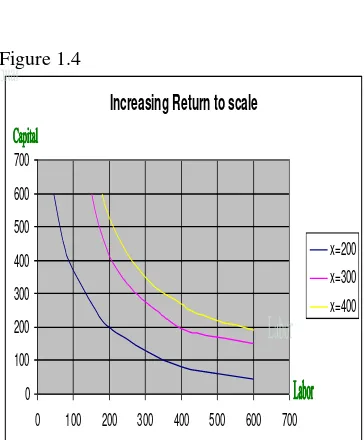
where, Y is related to product or service (output), K is related to capital, L is related to labor, and exponent ά and ß represent production parameters The value of the exponent ά and ß each should be greater than null but less than one (0 < ά < 1; 0 < ß < 1). The value of (ά + ß) in this function is particularly important to determine the return to scale. If (ά + β) is greater than one there are increasing return to scale; if (ά + ß) is equal to zero the return to scale is constant; and if (ά + ß) is less than one, there are decreasing in the return to scale.
Figure 1.2
Figure 1.3
Figure 1.4
Figures 1.2, 1.3, and 1.4 The illustration of Cobb-Douglas production function where labor and capital are input variables by Ruby (2003).
The facts show that the production function of Cobb-Douglas form has been widely used in the economics literature and has empirically supported long run property. For example used Cobb-Douglas production function to measure the China’s capital and productivity using financial resources; used this form to estimate the US industry-level capital labor substitution elasticity, and their estimates provide support for using the Cobb-Douglas specification as a transparent starting point in parameterizing applied
model and should be useful for researchers working on stimulation and sensitivity analysis. used a Cobb-Douglas specification that includes the capital stock and the labor force, as well as the average age of physical capital and the mean years of education to account for the quality of capital and labor, respectively.
Inefficiency. There are three main parametric frontier approaches. The stochastic frontier approach (SFA) – sometimes also referred to as the econometric frontier approach – specifies a functional form for the cost, profit, or production relationship among inputs, outputs, and environmental factors, and allows for random error. SFA posits a composed error model where inefficiencies are assumed to follow an asymmetric distribution, usually the half-normal, while random errors follow a symmetric distribution, usually the standard normal. The logic is that the inefficiencies must have a truncated distribution because inefficiencies cannot be negative. Both the inefficiencies and the errors are assumed to be orthogonal to the input, output, or environmental variables specified in the estimating equation. The estimated inefficiency for any firm is taken as the conditional mean or mode of the distribution of the inefficiency term, given the observation of the composed error term. The half-normal assumption for the distribution of inefficiencies is relatively inflexible and presumes that most firms are clustered near full efficiency. In practice, however, other distributions may be more appropriate.
Some financial institution studies have found that specifying the more general truncated normal distribution for inefficiency yields minor, but statistically significant, different results from the special case of the half-normal (Berger and DeYoung, 1996). A similar result using life insurance data occurred when a gamma distribution, which is also more flexible than the half-normal, was used. However, this method of allowing for flexibility in the assumed distribution of inefficiency may make it difficult to separate inefficiency from a random error in a composed-error framework, since the truncated normal and gamma distribution may be close to the symmetric normal distribution assumed for the random error.
The distribution-free approach (DFA) also specifies a functional form for the frontier, but separates the inefficiencies from random error in a different way. Unlike SFA, DFA makes no strong assumptions regarding the specific distributions of the inefficiencies or random errors. Instead, DFA assumes that the efficiency of each firm is stable over time, whereas random error tends to average out to zero over time. The estimate of inefficiency for each firm in a panel data set is then determined as the difference between its average residual and the average residual of the firm on the frontier, with some truncation performed to account for the failure of the random error to average out to zero fully. With DFA, inefficiencies can follow almost any distribution, even one that is fairly close to symmetric, as long as the inefficiencies are nonnegative. However, if efficiency is shifting over time due to technical change, regularly reform, the interest rate cycle, or other influences, then Constant Return to scale
0 100 200 300 400 500 600 700
0 100 200 300 400 500 600 700
x=100 x=200 x=300 x=400
Decreasing return to scale
0 100 200 300 400 500 600 700
0 200 400 600 800
x=200
x=300
x=400
Increasing Return to scale
0 100 200 300 400 500 600 700
2 Marthen Sengkey
DFA describes the average deviation of each firm form the best average-practice frontier, rather than true
efficiency at any one point in
time.Lastly, the thick frontier approach (TFA) specifies a functional form and assumes that deviations from predicted performance value within the highest and lowest performance quartiles of observations (stratified by size class) represent random error, while deviations in predicted performance between the highest and lowest quartiles represent inefficiencies. This approach imposes no distributional assumptions on either inefficiency or random error, except to assume that inefficiencies differ between the highest and lowest quartiles, and that random error exists within these quartiles. TFA itself does not provide exact point estimates of efficiency for individual firms but is intended instead to provide an estimate of the general level of overall efficiency. The TFA reduces the effect of extreme points in the data, as can DFA when the extreme average residuals are truncated (Berger and Humphrey 1997; Bauer et al 1993).
McDonell and Rubin (1991) identify sales of deposit and lending products as one of their critical success dimensions. There are two well-recognized approaches to modeling bank behavior known as intermediation and production. The intermediation approach posits deposits as being converted into loans.
Deposits are listed as input because banks buy deposits and other funds to make loans and investments. Deposits are basically considered as the raw materials of a financial institution and are measured by their total funds acquisition cost only. The asset approach stated that the primary role of financial institutions as creators of loans. In essence, this stream of thought is a variant of the intermediation approach, but instead defines outputs as the stock of loan and investment assets. Athanassopoulus (1998) categorized the output variables into four (4) categories as follows: type of new accounts (liability sales), loans and mortgages, financial products, and the number of credit cards sold.
The conceptual framework of this study has taken banks as intermediaries, where the primary function of the bank is to borrow funds from depositors and lend these funds to others for profit (Colwell and Davis, 1992). From this perspective, deposits are "inputs" and loans are "outputs."
Stated that environment variables are ownership (public/private, corporate, non-corporate), location (population, density, and average customers size), labor (union power), and government intervention (regulation).
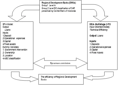
Conceptual Framework
The conceptual framework of the study is shown below: Figure 4. Research Paradigm
SFA Model: Output:
Loans
Inputs:
1.Deposit
2.Operational expenses 3.Capital
4.Fixed assets
Dummy Variables: 1. Government Intervention 2. Ownership
3. Location 4.ABC classification
The efficiency of Regional Development
Banks
Regional Development Banks (DMUs)
Group1 Level A
Group 2 Level BC classification of CAR prescribed by Central Bank of Indonesia.
DEA- Multistage (VRS Input Oriented Model): Technical Efficiency
Output: Loans
Inputs: 1.Deposits
2.Operational expenses 3.Capital
4.Fixed Assets
The DEA and SFA approaches are used to assess the productive efficiency of the banks’ management to maximize their loans as related to deposits, total expenses, capital, and fixed assets. Furthermore, both approaches are used to compute a comparative ratio of outputs to inputs for each unit, which is reported as the relative efficiency score. The efficiency score is usually expressed as either a number between zero and one or 0 and 100 percent. A decision-making unit with a score less than one is deemed inefficient relative to other units. In order to avoid a potential problem with DEA, operational performance through DEA can be complemented by ratio analysis that measures financial performance of a bank.
Efficiency performance was measured by DEA-Multistage (input oriented VRS model) and SFA. The dependent variable here is total loan, and the independent variables are deposits, total operating expenses, fixed assets and capital, which are the controllable variables by the management. The SFA model also investigates whether the technical inefficiency of regional development bank’s operational performance is affected by government intervention, ownership, location and ABC classification prescribed by Central Bank of Indonesia.
Further analysis is developed to determine whether there is a correlation between DEA model and SFA model. Spearman rank correlation is a tool to evaluate correlation of DEA efficiency rank and SFA efficiency rank. These combined models are employed generally to examine the performance management of regional development banks in Indonesia during the period 1994-2004.
Scope and Limitation of the Study. This study is limited to regional development banks in Indonesia over the time period 1994 to 2004. In this study, 26 regional development banks were categorized into the ABC classification of CAR prescribed by Central Bank of Indonesia. The main data sets gathered from the Institutions’ audited annual financial statement reports and statistical reports which were available from the Balitbang (Development Research Agency) located in Jakarta, Indonesia. Variables of off-balance sheet were not included in this study because of limited information. Storbeck, (1999) stated that some of the difficulties in obtaining overall efficiency measures in banking applications stem from data availability. First, banks' databases are often organized to accommodate traditional accounting procedures and do not lend themselves easily to the combined analysis of marketing, financial, and operational data. Second, competitor banks are not eager to share comparative data. Benchmarking among branches of different banks is virtually impossible in this environment. Finally, although one can obtain some data from central bank or from independent market-research agencies, these data allow, at best, comparisons of the bank's overall position vis-à-vis national or regional averages.
The variables used in this study were deposits, total operating expenses, capital, fixed assets, loan, government intervention, ownership, location and
ABC classification of CAR prescribed by Central Bank of Indonesia. Furthermore, the methods used were DEA multistage (input- oriented VRS model) SFA, and statistical tool such Spearman Rank Correlation Coefficient.
Null Hypotheses. Seven major null hypotheses were tested:
H01: The efficiency performances of Indonesia’s
regional development banks are consistent over the period.
H02: There are no input savings and
output deterioration of bank’s deposit, operational expenses, capital, fixed assets, and loan.
H03: There is no significant relationship between
loans with the following variables:
Deposit, Operating expenses, Capital, Fixed assets. H04: There is no relationship between
technical inefficiency effects in the production process with the following environmental variables: Government intervention
Ownership Location
ABC classification of CAR prescribed by Central Bank of Indonesia
H06: There is no correlation between
DEA and SFA efficiency results.
The rejection of these null hypotheses and evidence are found in Chapter 4.
RESEARCH METHODOLOGY
This study used the descriptive quantitative research design, using mathematical models of performance analysis in a panel data set of 26 regional banks in Indonesia. Two well-known frontier approaches were used. Firstly, the non-parametric but deterministic approach, DEA (multi-stage) was used to examine the efficiency performance of regional banks. Secondly, the parametric estimation known as SFA was used to evaluate the relationship of loans to deposit, total operational expenses, capital, and fixed assets and to test whether there is a presence of technical inefficiency effects in the model.
The third model used was the combination of Stochastic and DEA models as a new un-researched area in performance analysis, especially in banking. Using this model, the possible linkage between DEA and SFA efficiency scores were tested.
The general performance of Indonesia’s regional development banks was evaluated over the time period 1994-2004, using time series-analysis and panel data. The total sample was comprised of 26 state banks for 11 years or 286 total observations. This total observation reflected a long-run analysis that could yield more credible and unbiased investigation of a banking performance.
DATA AND VARIABLES
6 Marthen Sengkey
included all countrywide regional development banks, owned by 26 provinces in Indonesia. The time period covered from 1994 to 2004 was selected based on the availability and completeness of the data of audited financial reports. As stated in Chapter 1 under the consolidation period (1991–1997), Bank Indonesia adopted an open bank resolution strategy during this period only and therefore, data became publicly accessible and available.
There were four (4) independent variables or input data and one (1) dependent variable or output data to evaluate the efficiency of the regional development banks. As providers of financial services, banks use mainly capital and labor to produce loans, deposits, referrals to auxiliary services, and so forth. In this study, banks act as intermediaries where the primary function of the bank is to borrow funds from
depositors and lend these funds to others for profit (Colwell and Davis, 1992). Thus, this study used the intermediary approach in the banking performance. From this perspective, deposits are "inputs" and loans are "outputs." However, Berger and Humprey (1997) from a production approach perspective, banks are modeled as providing service to accounts holders so labor and physical capital as inputs and transaction and documents processing are treated as outputs. This study, on the other hand, considered banks as an intermediary of funds between savers and borrowers so inputs are sources of funds and loan as an output. The number of Indonesia’s regional development banks is shown in Table 3.1 below:
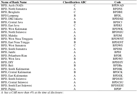
Table 1. Regional Development Banks
Name of Bank Name Classification ABC Code
BPD, Aceh (NAD) C BPDNAD
BPD, North Sumatera A BPDNS
BPD, Bengkulu C BPDBE
BPD Lampung B BPDL
BPD, DKI Jakarta A BPDDKI
BPD, Central Java B BPDCJ
BPD, East Java C BPDEJ
BPD, West Kalimatan A BPDWK
BPD, North Sulawesi A BPDNSU
BPD, Maluku A BPDM
BPD, West Nusa Tenggara B BPDWNT
BPD, East Nusa Tengga B BPDENT
BPD, West Sumatera C BPDWS
BPD, South Sumatera A BPDSS
BPD, Jambi A BPDJ
BPD, Pekanbaru-Riau A BPDR
BPD, West Java B BPDWJ
BPD, DIY A BPDDIY
BPD. Bali B BPDBa
BPD, South Kalimantan A BPDSK
BPD, Central Kalimantan B BPDCK
BPD, East Kalimantan A BPDEK
BPD, South Sulawesi A BPDSSU
BPD, Central Sulawesi A BPDCSU
BPD, South East Sulawesi A BPDSESU
BPD, Papua A BPDP
A has a CAR more than 4% at the time of disclosure;
B has a CAR less than 4% but greater than – 25% at the time of disclosure; C has a CAR less than – 25% at the time of disclosure.
Variables . This study used one (1) output variable and four (4) input variables to evaluate bank’s efficiency through the DEA multistage model (input oriented VRS technology). The output variable is total loans and input variables are (1) total deposits, (2) total operational expenses, (3) capital, and (4) total fixed assets.
Total loan composed of loan of rupiah currency (related parties and third parties) and loan of foreign currency (related parties and third parties). Then, total deposits composed of demand deposits, saving deposits, time deposits, and certificate deposits.
All those variables were stated in Indonesian currency (rupiah) in millions. These variables are chosen based on studies taking intermediation approach to banking performance.
According to commercial banks are financial intermediaries that supply financial service to surplus and deficit units. Most bank assets are financial in nature, consisting primarily of money owed by such non-financial economic units as households, business, and government. Furthermore, commercial banks issue contractual obligations, primarily in deposit or borrowing form, to obtain the funds to purchase these financial assets. He also stated that the role of commercial banking is to fill the diverse desires of both the ultimate borrowing and lenders in the economy.
McDonell and Rubin (1991) identified sales of deposit and lending products as one of their critical success dimensions. There are two well-recognized approaches to modeling bank behavior known as intermediation and production. The intermediation approach posits deposits as being converted into loans. Deposits are listed as input because banks buy deposits and other funds to make loans and investments. Other key inputs are operating and interest costs (Athanassopoulos, 1998). Under the intermediation approach, performance is assessed using as inputs such as total operating and interest costs. The intermediation approach uses outputs measured in dollars. However, there is no consensus on the variables that should be used to measure bank branch performance so far (Ibid.).
Furthermore, in addition to inputs and outputs, the study also used the exogenous variables, that are, dummy variables in the SFA model. Dummy variables (z) are government intervention, ownership, location of banks, and ABC classification prescribed by the Central Bank of Indonesia.
DEA – Multistage Model (Input-oriented VRS technology). DEA was originally introduced by Charnes et al., (1978) and is a non-parametric linear programming approach, capable of handling multiple inputs as well as multiple outputs. DEA assumes that the inputs and outputs have been correctly identified. Usually, as the number of inputs and outputs increase, more DMUs tend to get an efficiency rating of 1 as they become too specialized to be evaluated with respect to other units. On the other hand, if there are too few inputs and outputs, more DMUs tend to be comparable. In any study, it is important to focus on correctly specifying inputs and outputs. According to Kruger (2003), DEA is a local method in that calculates the distance to the frontier function through a direct comparison with only those observations in the samples that are most similar to the observation for which the inefficiency is to be determined.
The piece-wise linear form of non-parametric frontier in DEA can cause a few difficulty in efficiency measure. The problem arises because of the sections of the piece-wise linear frontier, which run parallel to the axes which do not occur in most parametric function (Coelli et al., 1998).
Environment is the factor which could influence the efficiency of a firm, where such factors are not traditional inputs and are assumed not under the control of manager. Some examples of environmental variables include ownership, location, labor, and government regulation. If the values of the environmental variable can be ordered from the least to the most detrimental effect upon efficiency, then the approach of can be followed. On the other hand, if there is no natural ordering of the environmental variable then one can use a method proposed by.Charnes et al., (1978) stated that the DEA technique as an efficiency measure of production unit by its position relative to the frontier of the best performance, established mathematically by the ratio of weighted sum of outputs to weighted of sum of inputs; different decision making units (DMU) can be compared based on productivity and efficiency. A common practice in this case is to run DEA where all the inputs are treated as controllable and then regress the emerging efficiency scores on non-discretionary inputs.
In this study, the multistage DEA model was utilized to compute the total efficiency scores. According to Coelli et al., (1998, p. 150), the constant returns to scale (CRS), DEA model is only appropriate when the firm is operating at an optimal scale. Some factors such as imperfect competition, constraints on finance, banking, corruption, political crisis etc. may cause the bank to be not operating at an optimal level in practice.
The fall of Soeharto and five (5) years after the financial crisis, Indonesia is still struggling to deal with economic restructuring and recovery, political transition, decentralization and redefining national identity. Moreover, the Asian financial and economic crisis of 1997-1998 hit the country hardest, which caused its real GDP declined by 13 percent in 1998 as its banking and modern corporate sectors collapsed in the wake of short-term capital outflows. Corporate debts remain largely unreconstructed, bank lending is limited, the government owns or controls most of the banking system and substantial business assets, fiscal sustainability is questionable, inflationary pressures are strong and investment climate is unattractive.
To considerall these environmental factors that may affect the banking performance in Indonesia, this study adopted DEA model of variable returns to scale (VRS). Due to the consequence of the heavy intervention by the government in banking system in Indonesia as mentioned earlier, bankers may well have been prevented from operating at the optimal level in their operation. Therefore, technical efficiency in this study is calculated using the input-oriented VRS model. The envelopment form ofthe input-oriented of CRS and VRS DEA model is specified as stated by Coelli et al. (1998, pp. 150, 151).
min ,
, :
st
y
i
y
0
,
x
i
x
0
8 Marthen Sengkey
SE
TE CRS
TE VRS
i i
i
(3.2)min ,
, :
st
y
y
i
0
x
i
x
0
N
1
'
1
0
(3.3)where θ is a scalar and λ is a N*1 vector of constants, N*1 is an vector of one.
In this study, θi is the technical efficiency score
for each bank, N is number of bank which is 26, λ is the lambda weight of each bank to the target or peer, y is the output variable (loan) and x is the input variables (deposit, total expenses, fixed assets, and capital). The efficiency score will satisfy if the value of θ is less and equal than one. If there is a difference in the CRS and VRS TE scores for a particular firm, then this indicates that the firm has scale inefficiency, and that the scale inefficiency can be calculated from the difference between CRS and VRS TE (Coelli et al., 1998, pp.134, 140, and 141). Furthermore, the nature of the scale inefficiencies for particular firm can be determined by seeing whether the non- increasing return to scale (NIRS) technical efficiency (TE) of NIRS TE score is equal to the VRS TE score. If they are unequal, then increasing return to scale exists for the firm. If they are equal, then decreasing return to scale applies. And if TECRS = TEVRS the firm is
operating under constant return to scale CRS (Coelli et al. 1998, pp.150- 151). The efficiency scores in this study were estimated, using the computer program known as Efficiency Measurement System -EMS.
Slacks. The piece-wise linear form of the non-parametric frontier in DEA can cause a few difficulties in efficiency measurement. The problem arises because of the sections of the piece-wise linear frontier which run parallel to the axes which do not occur in most parametric functions Coelli et al., (1998). Some authors argue that both the Farrell measure of technical efficiency (θ) and any non-zero input or output slacks should be reported to provide an accurate indication of technical efficiency of a firm in DEA analysis Coelli et al., (1998). They sated that the output slacks will be equal to zero if and only if Yλ-y1=0 and the input slacks will be equal to zero if and
only if θx1-Xλ=0 (for the given optimal values of θ
and λ).
Coelli et al., (1998) stated that there are two major problems associated with the second stage LP. The first and most obvious problem is that the sum of the slacks is maximized rather than minimized. Hence, it identifies not the nearest efficient point but the furthest efficient point. The second major problem associated with the second – stage approach is that is not invariant to unit of measurement. To avoid the two problems mentioned, the multi-stage DEA method was used. Coelli (1998) stated that the multi-stage method involves a sequence of radial DEA models and hence is more computationally demanding that the first-stage and second-stage methods. However, the benefits of the approach are that it identifies efficient projected points which have input and output mixes as similar as
possible to those of inefficient points, and that it also invariant to units of measurement. For a detailed explanation, see Coelli et al., (1998).
Stochastic Frontier Analysis. The SFA method provides the means to estimate cost efficiencies. Cost efficiency consists of two components: technical efficiency, which reflects the ability of the firm to obtain maximum output from a given set of inputs, and an allocative efficiency, which reflects the ability of the firm to use the inputs in optimal proportions, given by their respective prices. The SFA model involves the estimation of a cost frontier, as a function of outputs and input prices, where deviation from the frontier are assumed to be related to cost inefficiency and statistical noise (Greene and Segal, 2004).
The SFA method can statistically test hypotheses and construct confidence intervals, allowing for random error. Stochastic frontier analysis is an econometric frontier approach that specifies a functional form for the cost, profit, or production relationship among inputs, outputs, and environmental factors, and allows for random error. SFA posits a composed error model where inefficiencies are assumed to follow an asymmetric distribution, usually the half-normal, while random errors follow a symmetric distribution, usually the standard normal (Berger et al.,1997).
The following stochastic frontier model can be run:
L y
n(
it)
x
it
v
it
u
it,
i=1,…,N; t=1,…,T(3.4)
u
it
exp
n t
T
u
i (3.5)where yit denotes the output for the ith bank at tth
time period; xit denotes a (1*K) vector of value of
inputs and other appropriate variables associated with a suitable functional form (e.g., the Cobb-Douglas model); β is a (K*1) vector of unknown scalar parameters to be estimated; the vits are random errors;
the uits are the technical inefficiency effect in the
model (Coelli, et al., 1998).
In this study, y is total loan, xi are deposit,
operational expenses, capital and fixed assets. While uit is other environmental variable that is not included
in the input or output variables, which influence the result of technical efficiency score.
To evaluate the effects of government intervention, ownership, location and ABC classification described by the Central Bank of Indonesia, of the Indonesia’s regional development banks on technical inefficiency, the uits are
Bank of Indonesia represents the technical inefficiency term. Where u it is defined mathematically as:
uit= δ0+ δ1z1it+ δ2 z2 it+ δ3 Z3 it +δ4z4 it Dit (3.6)
where :
Z1it = represents the government intervention i – th in
the t –th year of observation;
Z2 it = represents the bank’s ownership i – th in the t –
th year of observation;
Z3 it = represents the bank’s location i – th in the t-th
year of observation;
Z4 it = represents the ABC classification of CAR prescribed by central bank of Indonesia i-th in the t-th year of observation;
Dit isdummy variable having value one and zero if the
i – th bank in the t - th year of observation include the government intervention.
The computer program software known as Frontier 4.1 (Coelli, 1996) was usedto find maximum likelihood estimates of a subset of the stochastic frontier production functions.
Strength of SFA. The SFA method can statistically test hypotheses and construct confidence intervals allowing for random errors.
Weaknesses of SFA. Some weaknesses of SFA are follows: the selection of a distributional form for the inefficiency effects may be arbitrary and the production technology must be specified by a particular functional form (Coelli et al., 1998); Eventhough SFA can statistically test hypotheses and construct confidence intervals allowing for random errors, it may lose some flexibility in model specification.
Strengths of DEA. DEA modeling allows the analyst to select inputs and outputs in accordance with a managerial focus. Furthermore, the technique works with variables of different units without the need for standardization (e.g. dollars, number of transactions, or number of staff). That is, DEA does not assume a particular production technology or correspondence. The importance of this feature of DEA is that a bank's efficiency can be assessed based on other observed performance. As an efficient frontier technique, DEA identifies the inefficiency in a particular DMU by comparing it to similar DMUs regarded as efficient, rather than trying to associate a DMU's performance with statistical averages that may not be applicable to that DMU.
Assessment of operational performance through DEA can be complemented by ratio analysis that measures financial performance of a branch. DEA is that it allows management to nominate the inputs and outputs entering the analysis. DEA allows inputs to be classified as either controllable or uncontrollable by management. This facilitates an analysis where performance can be interpreted in the context of uncontrollable environmental conditions. DEA models can offer much potential for a significant advance in the comparative analysis of financial institutions by enabling the concurrent study of the multiple variables that affect bank efficiency over time (Bauer et al., 1997)
The limitation of DEA as stated by Coelli et al., (1998) are the following: measurement error and other noise may influence the shape and position of the frontier; the exclusion of an important input or output can result in biased results; and the addition of extra
input or output cannot result in a reduction in the TE scores.
The principal disadvantage of DEA is that it assumes data to be free of measurement error. When the integrity of data has been violated, DEA results cannot be interpreted with confidence. While the need for reliable data is the same for all statistical analysis, DEA is particularly sensitive to unreliable data because the units deemed efficient determine the efficient frontier and thus, the efficiency scores of those units under this frontier. For example, an unintended reclassification of the efficient units could lead to recalculation of efficiency scores of the inefficient units. This potential problem with DEA is addressed through stochastic DEA designed to account for random disturbances. Two recent examples in this area are.
Another caveat of DEA is that those DMUs indicated as efficient are only efficient in relation to others in the sample. It may be possible for a unit outside the sample to achieve a higher efficiency than the best practice DMU in the sample. Another way of expressing this is to say that an efficient unit does not necessarily produce the maximum output feasible for a given level of input.
Spearman Rank Correlation Coefficient. To assess the correlation between DEA- the non-parametric approach and SFA- the non-parametric analysis in this study, Spearman ranks correlation coefficient was used to address objective (6). The Spearman rank correlation when coefficient
( Rrank ) is used to determine whether there is a
significant difference between DEA efficiency rank and SFA efficiency rank (Berger and Humphrey, 1997). They stated that some studies found significant different relationship between the findings of different techniques, while others find strong relationships. The test of independent sample, paired sample, and spearman rank correlation are computed through Statistical Program for Social Sciences (SPSS) version 11.5.
10 Marthen Sengkey
r
d
n n
s
i
1
6
1
2
2
(3.10)
where: diis the difference between the rankings for
each observation and n is the sample size of the observation (Webster, 1992). The quantity rs called the
linear correlation coefficient, measures the strength and the direction of a linear relationship between the pairs of data.
The value of rsis such that -1 < r s< +1. The +
and – signs are used for positive linear correlations and negative linear correlations, respectively. Positive correlation: If the comparable variables have a strong positive linear correlation, where rs is close to
+1. And if rs value is exactly +1 indicates a perfect
positive correlation. On the other hand, a negative correlation occurs: If x and y have a strong negative linear correlation, rs is close to -1. And if rs value of
exactly -1 indicates a perfect negative correlation. No correlation: If there is no linear correlation or a weak linear correlation, rs is close to 0. A value near zero
means that there is a random, nonlinear relationship between comparable variables such independent and dependent variables. A perfect correlation of ± 1 occurs only when the data points all lie exactly on the line if we plot the result on the graphic.
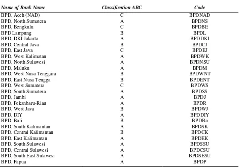
Data Sources
Table 2. Regional Development Banks
Name of Bank Name Classification ABC Code
BPD, Aceh (NAD) C BPDNAD
BPD, North Sumatera A BPDNS
BPD, Bengkulu C BPDBE
BPD Lampung B BPDL
BPD, DKI Jakarta A BPDDKI
BPD, Central Java B BPDCJ
BPD, East Java C BPDEJ
BPD, West Kalimatan A BPDWK
BPD, North Sulawesi A BPDNSU
BPD, Maluku A BPDM
BPD, West Nusa Tenggara B BPDWNT
BPD, East Nusa Tengga B BPDENT
BPD, West Sumatera C BPDWS
BPD, South Sumatera A BPDSS
BPD, Jambi A BPDJ
BPD, Pekanbaru-Riau A BPDR
BPD, West Java B BPDWJ
BPD, DIY A BPDDIY
BPD. Bali B BPDBa
BPD, South Kalimantan A BPDSK
BPD, Central Kalimantan B BPDCK
BPD, East Kalimantan A BPDEK
BPD, South Sulawesi A BPDSSU
BPD, Central Sulawesi A BPDCSU
BPD, South East Sulawesi A BPDSESU
BPD, Papua A BPDP
A has a CAR more than 4% at the time of disclosure;
B has a CAR less than 4% but greater than – 25% at the time of disclosure; C has a CAR less than – 25% at the time of disclosure
.
The data used in this study were available publicly from the agency for research and development (BALITBANG) located in Jakarta, Indonesia. Audited financial statements and other statistical reports of banks were acquired. From these statements, it was possible to collect data on four (4) main input variables (deposits, operating expenses, capital and total fixed assets) and one (1) output variable (loans,) for the period 1994-2004. Since data were archived on microfilm database, the collection process proved excessively time-consuming. Data related to literature reviews, tools for analyzing, and
references referred to the journals, working papers (from Internet), books, and reports available at Adventist International Institute of Advanced Studies (AIIAS) library, and Adventist International Institute of Advanced Studies (AIIAS)’s on line data base.
RESULTS AND DISCUSIONS
DEA was used in this study to compare the efficiency estimates among the Indonesia’s regional development banks and evaluate the input usage/savings and output deterioration for each bank’s performance. The key advantage of DEA over other methods of performance evaluation is that it allows one to consider a number of outputs and inputs simultaneously, regardless of whether all the variables of interest are measured in common units (Sexton, 1986).
In this evaluation process, the study used four (4) variables (deposit, operating expenses, capital, and fixed assets) as inputs and loans as output. The result of efficiency score and inputs slacks were summarized in Table 3.
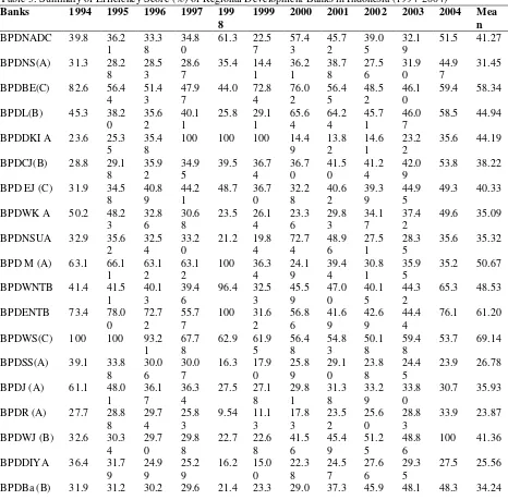
Results reveal that bank, which has the highest efficiency estimate score among 26 banks is BPDWS (69.14 percent), which means BPDWS could possibly reduce the usage of all inputs (deposit, operating expenses, capital and fixed asset) by 30.86 percent (1-0.6914) without reducing the current output. This same bank had an efficiency score of 100 percent in
1994 and 1995, which means that it did not incur input excesses. Eventhough, BPDWS showed a decline from 93.21 percent in 1996 to 53.7 percent in 2004, this bank still posted the highest efficiency performance for the entire evaluation period.
BPDDKI posted an efficiency score of 100 percent from 1997 to 1998, however, this bank occupied the eighth rank in terms of efficiency estimate score due to its very low
efficiency scores of 28.17 percent (1994-1996) and 27.35 percent (1997-2004). The banks that have the second and third ranks with a higher efficiency estimate score are BPDENT and BPDBE with scores of 61.20 percent and 58.34 percent, respectively. Results imply that BPDENT and BPDBE could reduce their given inputs by 38.80 percent and 41.66 percent, respectively without reducing the present output. Otherwise, the bank that has the lowest efficiency score is BPDP with a 19.14 percent efficiency estimate score. This means that this bank has been wasting in using all the inputs by 80.86 percent.
Table 3. Summary of Efficiency Score (%) of Regional Development Banks in Indonesia (1994-2004)
12 Marthen Sengkey
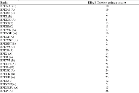
Table 4. Rank Based of Efficiency Estimates Score (DEA) of Regional Development Banks in Indonesia (1994-2004)
Banks DEA Efficiency estimates score
BPDNAD(C) 10
Determine the input usage/savings and output deterioration for each bank’s performance (DEA approach)
Input slacks. The summary of input slacks over the evaluation period 1994 to 2004 of this study is shown in Table 4. Keep in mind that input slacks refer
to input surplus or excess that a bank need to reduce to be efficient.
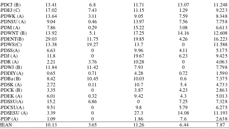
Table 5. Summary of Input Slacks (%) of Regional
Development Banks in Indonesia (1994-2004)
BANKS DEPOSIT OPRT.EXPENSES CAPITAL FIXED ASSETS MEAN
BPDNA(C) 17.36 2.54 10.27 10.49 10.165
BPDNS (A) 10.25 1.71 12.57 15.17 9.925
BPDBE (C) 14 2.81 7.12 10.16 8.523
BPDL(B) 16.03 0 17.01 13.16 11.550
BPDCJ (B) 13.41 6.8 11.71 13.07 11.248
BPDEJ (C) 17.02 7.43 11.15 1.29 9.223
BPDWK (A) 13.64 3.11 9.05 7.59 8.348
BPDNSU (A) 9.04 0.46 13.97 7.56 7.758
BPDM (A) 7.86 0.29 15.22 3.08 6.613
BPDWNT (B) 13.92 5.1 17.25 14.16 12.608
BPDENT(B) 29.03 11.75 19.85 4.26 16.223
BPDWS(C) 13.38 19.27 13.7 0 11.588
BPDSS(A) 6.63 0 9.96 4.11 5.175
BPDJ (A) 11.8 0 19.67 6.23 9.425
BPDR (A) 2.21 3.76 10.28 0 4.063
BPDWJ (B) 11.84 11.42 7.93 0 7.798
BPDDIY(A) 0.65 0.71 4.28 0.72 1.590
BPDBa (B) 8.42 10.45 10.03 0.6 7.375
BPDSK (A) 2.72 0.11 10.7 5.4 4.733
BPDCK (B) 3.35 0 3.87 4.23 2.863
BPDEK (A) 6.01 0.32 9.42 4.3 5.013
BPDSSU(A) 15.2 6.86 0 7.25 7.328
BPDCSU(A) 9.51 0 9.8 5.79 6.275
BPDSESU (A) 3.39 0 27.3 14.08 11.193
BPDP (A) 1.09 0 1.86 7.6 2.638
MEAN 10.13 3.65 11.26 6.44 7.87
Table 5 shows in detail how much each bank input could be reduced to reach the best practice frontier (efficiency level). In terms of deposit as an input, all banks incurred input slacks. Banks with a higher input slack have a lower efficiency performance. The result shows that the most inefficient bank is BPDENT, with the highest deposit slack of 29.03 percent, followed by BPDNAD of 17.36 percent, BPDEJ of 17.02 percent, and BPDL of 16.03 percent, all excesses in deposits. To become efficient, banks such as BPDENT needs to reduce its deposit of 29.03 percent, BPDNA of 17.36 percent, BPDEJ of 17.02 percent, and BPDL of 16.06 percent. Otherwise, bank which has the lowest slack of deposit is BPDIY. Analytically, this bank needs only to reduce its deposit of 0.65 percent to be a 100 percent efficient.
The second input is operating expenses. This study found out that there are eight (8) banks that do not need to reduce their operating expenses due to zero slack result. Those banks are the following: BPDL, BPDKI, BPDSS, BPDJ, BPDCK, BPDCSU, BPDSESU and BPDP. On the other hand, BPDWS, which is known as the top performer in the efficient estimate score, has the highest slack in operating expenses of 19.27 percent, compared with the highest efficiency estimate score of 69.14 percent.
The third input variable is capital. The result shows that most of the banks have capital surpluses, except for BPDSSU, which has a zero slack. There are three banks which have the highest input slack of capital among 26 banks. Those banks are the following: BPDSESU, with a capital surplus of 27.30 percent, BPDENT of 19.85 percent, and BPDJ of 19.67 percent. In other words, these banks need to reduce their capital as much as their slack rating without reducing their current output. The last input variable is fixed asset. There are two (2) banks that posted zero slack. Those banks are the following: BPDR and BPDWJ. BPDR occupied the third rank with the lowest slack in terms of deposit, eleventh rank
in terms of operating expense slacks, and the fourteenth rank in terms of capital slacks. While BPDWJ has the sixteenth rank in terms of deposit slacks, the eighth rank in the highest slack in terms of operating expenses, and the sixth rank in the lowest slack in terms of capital. By using the DEA approach, the result shows that no bank in the sample has a consistent efficiency performance in terms of efficiency or inefficiency score. The result of DEA approach shown that, none of the banks has a consistence performance for all variables used in DEA.
Table 5 shows that, on average, the highest slacks of all input variables were posted by BPDENT (12.68 percent) while the lowest slacks were posted by BPDIY (1.59 percent). BPDIY has managed to utilize efficiently its deposit, operating expenses, capital, and fixed assets to the production of loans (as an output): it calls for a reduction of all inputs by 1.59 percent only to become efficient. Furthermore, results imply that BPDENT needs to reduce 12.68 percent, on average, its input variables (deposit, operating expenses, capital, and fixed assets) to become efficient. However, Table 4.3 shows that none of the banks incurred output slack, because the output slacks of all banks are zero. Thus, the presence of input slacks in deposit, operating expenses, capital and fixed assets did not effect to produce the loan as an output.
12 Marthen Sengkey
three (3) input variables to produce loan as an output. This result contradicts with the study of Avkiran (1999) that evaluated the efficiency of 65 banks in
Australia, wherein, a rise in inputs will lead to a proportionate rise in outputs.
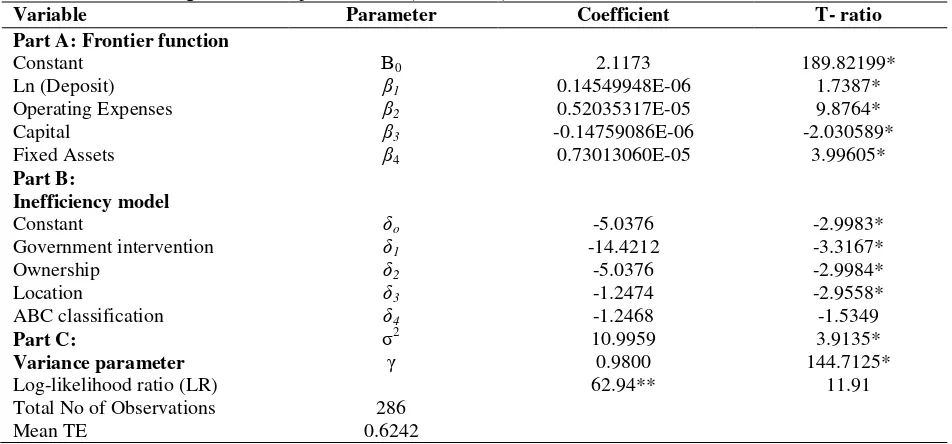
Table 7. Maximum-Likelihood Estimates of Parameters of the Cobb-Douglas Stochastic Frontier Production Function of Regional Development Banks (1994-2004)
Variable Parameter Coefficient T- ratio
Part A: Frontier function
Constant Β0 2.1173 189.82199*
Ln (Deposit) β1 0.14549948E-06 1.7387*
Operating Expenses β2 0.52035317E-05 9.8764*
Capital β3 -0.14759086E-06 -2.030589*
Fixed Assets β4 0.73013060E-05 3.99605*
Part B:
Inefficiency model
Constant δo -5.0376 -2.9983*
Government intervention δ1 -14.4212 -3.3167*
Ownership δ2 -5.0376 -2.9984*
Location δ3 -1.2474 -2.9558*
ABC classification δ4 -1.2468 -1.5349
Part C:
Variance parameter
σ2
γ 10.9959 0.9800
3.9135* 144.7125* Log-likelihood ratio (LR)
Total No of Observations Mean TE
286 0.6242
62.94** 11.91
**significant. LR test of the one-sided error = 0.62945107E+02, with number of restrictions =6 (critical value at 5 % level=11.91 from Kodde and Palm (1986) table.
*significant. The t-ratio, which is set at 5% level, with a critical value of 1.645 (see t-distribution table).
Cobb-Douglas Stochastic Frontier Production. This study used stochastic frontier analysis to examine the relationship between bank loans (output) and the following input variables: (1) deposit, (2) operational expenses, (2) capital, and (4) fixed assets. Moreover, it was used to test whether there is technical inefficiency effects to the production process on banks output of loan by the following firm’s specific and environment variables: (1) government intervention, (2) ownership, (3) location, (4) ABC classification described by Central Bank of Indonesia.
The computation of the maximum likelihood estimation of the parameters in the Cobb-Douglas stochastic frontier model was derived by the aid of the FRONTIER Version 4.1 (Coelli, 1996). It used to select the worthy functional form and to determine the existence of the inefficiencies in the model. The Cobb-Douglas function is chosen over the translog function, because the log likelihood value obtained using the translog is lower than that of the Ordinary Least Square (OLS).
The null hypothesis of the Cobb – Douglass function form is that, there is no technical inefficiency effect in the model, which can be stated as: γ = δ0 = δ1
= δ2= δ3 = δ4 = 0. To test whether the hypothesis is
accepted or rejected, the likelihood ratio (LR) test of the one-sided error was compared with the critical value from Table 1. The result shows that the LR test of 62. 94 is greater than the critical value of 11.91 at 5 percent level, with a degree of freedom of six (6). Thus, the null hypothesis is rejected which means that there is a technical inefficiency in the model (Coelli, 1998) (see Table 4.5.) In the process of banks producing loan as an output by input variables of deposit, operating expenses, capital, and fixed assets,
they were influenced by the environment variables as the following: (1) government intervention, (2) ownership, (3) location, and (4) ABC classification described by the Central Bank of Indonesia.
Analysis of Beta Parameters. The beta parameters indicate the association between banks’ technical efficiency (TE) with the inputs variables of deposit, operating expenses, capital and fixed assets. It may have a direct or inversed relationship. Table 4.5 shows the summary of beta parameters, delta parameters, gamma, and likelihood ratios. This study found out that beta zero represents the constant estimated coefficient of input variables has a positive sign and statistically significant, indicating that in general, there are fixed efficiency increase when banks used deposit, operating expenses, capital, and fixed assets to produce loan. The positive relationship means that the technical efficiency of the banks increases when deposit, operating expenses, capital and fixed assets increase. The estimated coefficient of bank’s deposit (β1) has a positive sign and statistically
significant, indicating that used of more deposits increased significantly the efficiency of the banks to produce loan. It is consistent with the function of bank as intermediation, where bank collects fund from surplus side as a depositor and then invests that fund as a loan or other types of investment to get more earnings.
affirmed the study, where the Indonesia’s domestic banks’ efficiency increases as they used more bank’s deposit as an input.
The operating expenses have a significant positive influence to the efficiency of the bank. This result reveals that each dollar spends by the banks can increase its efficiency. It is contradiction with the theory that the higher operating expenses, the lower the operating income. However, today’s high competitiveness in the industry of financial institutions is causing difficulties to the bank to raise funds with the lower rate of interest to the depositor and creditors. Innovation, in the form of new deposit plans, service delivery methods, and pricing schemes, is rampant in banking today. Bankers who fail to stay abreast of changes in their competitors’ deposit pricing and market programs stand to lose both customers and profit (Rose, 1996). Whereas the result of this study shows that banks’ capital has a significant negative relationship with the bank efficiency. It implies that less use of capital in the operation increases significantly the technical efficiency of banks to produce loan. It contradicts with the requirement of the bank authorities of Indonesia, that increased loan should be backed-up with the adequate capital to prevent bank failure. Furthermore, according the Basle Agreement, each country is allowed to apply its own capital adequate ratio (CAR), using Basle Agreement as a basic minimum (Coyle, 2000). The association between deposit and operating expenses implies that the banks used more deposits as a source of funds and higher operating expenses to increase portfolio of loans and do not have to be covered by high capital as a back up for loan risks. This situation indicates that the management of the banks takes a high risk to lend the funds.
Finally, fixed asset in the efficiency function shows a significant positive relationship with the efficiency of banks to produce loan. It indicates that, the bank’s productivity increases significantly when more fixed assets are utilized as an input. The result of this study is consistent with the theory that the key profitability ratios in banking are ROE and ROA. Thus, ROA is primarily an indicator of managerial efficiency: it indicates how capably the management of the bank has been converting the institution’s assets into net earnings (Rose, 1996).
Analysis of Delta Parameter (Technical Inefficiency Effects) . Part B of Table 7 shows that delta 0 (general) has a negative sign, which is affected by those four (z) variables used in the study. The effect is negative and significant at 5 percent probability level. The government intervention to the banks has a significant negative effect on its technical inefficiency. The negative sign indicates that those banks without funds received from the bank authority (non-recapitalized banks) are more technically efficient than those banks that received funds (recapitalized banks). It is contradicted to the purpose of the government that by injecting funds, banks can improve their performance. A bank’s role and size are not the only determinants of how it is organized or how well it performs. Government regulation also has
played a major role in shaping the needs and diversity of banking organizations that operate around the globe (Rose, 1996).
The estimate coefficient in connection with ownership has the negative sign and significant at 5 percent probability level. This means that ownership has a statistically significant effect on technical inefficiency. The negative sign suggests that banks with less than 50 percent ownership are technically efficient. The ownership consists of central government, province government, municipal government and others. Fifty percent ownership means, it owned by the province government. Thus, the banks that have a percentage less than 50 percent is owned by province’s government are technically efficient compared with banks that have a percentage of more than 50 percent owned by the province government. The result indicates that an increase in the percentage ownership decreases the efficiency of the bank. The result is consistent with previous studies’ results that the ownership of the financial institutions has the influence over the productivity of the organization. Fama and Jensen (1985), and Mayers and Clifford (1986, 1988) argued that firms with alternative ownership structures differ in their operations and particularly in their cost of productions.
Moreover, the estimated coefficient of location is negative and statistically significant at 5 percent level. It indicates that those banks that located outside West Region of Indonesia are more technically efficient. Finally, the estimated coefficient of ABC classification described by the Central Bank of Indonesia is negative and suggests a negative effect on technical inefficiency but statistically not significant at 5 percent level. It suggests that those banks under BC classification are technically efficient than those under A classification. The new result is a contradiction to the Indonesia’s bank authority policy that those banks having CAR above the minimum requirement have a good performance. Also, according to Basle Agreement that each country is allowed to apply its own capital adequacy ratio using, the Basle Agreement as a basic minimum. In 1999 after the Asia’s financial crisis, the bank authority of Indonesia applied the minimum CAR of eight percent (8%).
In part C of Table 4.5 shows that the results of the parameters
s
v
2
2
2and
2/
s2, arerelated to the variance of the variables, vit and uit. The
result shows that the estimate for the