this PDF file MODIFIED ISING MODEL FOR GENERATING BINARY IMAGES | Halim | Jurnal Informatika 1 PB

(1)

Jurusan Teknik Informatika, Fakultas Teknologi Industri – Universitas Kristen Petra http://puslit.petra.ac.id/journals/informatics

MODIFIED ISING MODEL FOR GENERATING BINARY IMAGES

Siana Halim

Industrial Engineering Department, Petra Christian University Siwalankerto 121-131, Surabaya 60236, Telp, +62 31 298 3425

Email: halim@petra.ac.id

ABSTRACT: In this paper the Ising model is modified by considering its parameters as a vector that depends on the neighborhoods of the image’s pixels. We applied this modification for generating binary images, provided the original image is given. An example is exposed as a result of simulation using Gibbs sampler.

Keywords: markov random fields, ising model, gibbs distributions, gibbs sampler.

INTRODUCTION

Generating image is a part of the texture modeling. Basically, texture modeling can be classified to be two models, i.e., the deterministic models or the probabilistic ones. The deterministic models, usually rely on a heuristics procedure, e.g., Efros et.al. [4,5], Li Yi Wei [11]. On the other hand, the probabilistic models are mainly based on the random fields, e.g., Besag, [2,3], Geman and Geman [6,7], Paget [10], Winkler [12].

In this paper we used the Gibbs random field, in particular with the Ising model as its energy function, for generating an image. We modified the Ising model by considering its parameters as a vector that depends on the neighborhoods of image’s pixels.

MARKOV RANDOM FIELDS

To model a digital image as a realization of a Markov Random Field (MRF), we consider a finite index set S to be given and the elements s ∈ S denote

the pixels or sites of an image x. Assume that a finite set of discrete labels or gray scale value Ls ⊆ L is

given for every site s ∈S.

We denote the set of all images X = {Xs; Xs ∈ Ls,

s ∈ S } by χ

Definition 2.1: Neighborhood System

Let N denote a collection of subsets of S of the form N = {N(s) ⊂ S | s ∈ S}

N is called a neighborhood system for S if it satisfies (i) s ∉ N(s) ∀ s ∈ S

(ii) ∀ s,t ∈ S with s ≠ t

We have s∈N(t) ⇔ t∈N(s)

The sites t∈N(s) is called neighbors of s. We write

<s,t> if s and t are neighbors of each other.฀

In the case of a regular pixel grid the set of sites S

can be considered to be a subset of Z2, e.g., S = {(i,j) ∈ Z2

| -n ≤ i,j ≤ n}for a square lattice of size (2n+1) x

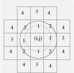
(2n+1). We define the neighbors of a pixel (i,j) on such a grid to be the set of nearby sites whose midpoints lie within a circle for radius c, i.e.,

N(i,j) := {(k,l) ∈ S | 0 < (k-i)2 + (l-j)2 ≤ c2}

To describe the kind of neighborhood, we define the order of a neighborhood with increasing c. The

first order neighborhood system for which c2 = 1, the

second order neighborhood system corresponds to c2 = 2 considers the eight nearest pixels to be neighbors and so on. We will denote these neighborhood systems by No, where o ∈{1,2,...}corresponds to the order.

Figure 1. Illustration of the neighborhood systems of order 1 to 4: The pixels having their midpoints within the smaller circle are first order (c_{= 1),}

pixels within the larger circle are second order neighbors (c = 2).

This system can be decomposed into subsets called a clique, which is going to be used in the next section, in this way.

(2)

JURNAL INFORMATIKA VOL. 8, NO. 2, NOPEMBER 2007: 115 - 118

116

Definition 2.2: Clique

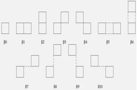
A subset C⊂ S is called a clique with respect to the neighborhood system N if either C contains only one element or if any two different elements in C are neighbors. We denote the set of all cliques by C . ฀

For any neighborhood system N we can decom-pose the set of all possible cliques into subsets Ci, i = 1,2,...,which contain all cliques of cardinality i, respectively.

Then we have C = Υ_iC_i with C1:= {{s}| s∈ S} being the set of all singletons, C2 :={{s1,s2} | s1,s2 ∈S

are neighbors}, the set of all pair-set cliques, and so on.

Figure 2. The different clique types with their asso-ciated clique parameters

Now, we can define a Markov random field (MRF) with respect to the neighborhood system N. A MRF with ∏ density the distribution of the whole image X and ∏s the marginal distribution of the gray

scale value Xs at pixel s ∈ S can be formulated as

∏s (xs|xr, r ≠ s) = ∏ (xs|xr, r ∈N(s),

s ∈ S, x ∈ χ (1)

An image is modeled by estimating this function with respect to a neighborhood system N.

GIBBS RANDOM FIELDS

To calculate the conditional probability in (1) we use the representation of random fields in the Gibbsian form, that is, we assume,

∏ = −

which are always strictly positive and hence random fields.

Such a measure ∏ is called the Gibbs Random Field (GRF) induced by the energy function, H, and the denominator Z is called the partition function. It is convenient to decompose the energy into the contri-butions of configurations on subsets of S.

Definition 3.1: Potential Function

A potential is a family {UA: A ⊂ S}of functions

We call U a neighbor potential with respect to a neighborhood system N if UA ≡ 0 whenever A is not a clique. The functions UA are then called as clique potentials. In the following we denote a clique potential by UC where C ∈ C.

Let ∏ be a Gibbs field where the energy function is the energy of some neighbor potential U with respect to a neighborhood system N that is

∏ = −∑

Then the local characteristics for any subset A ⊂ S

are given by

MODIFIED ISING MODEL

Many models for texture synthesis have been constructed via Markov Random Fields. Some of the famous models are the Ising Model, Binomial models and the Phi model can found in e.g. Winkler [12].

The models above work well for synthesizing random textures. The Phi model has been applied for tomographic image reconstruction by Geman [6], and also in segmentation of natural textured images, Geman and Graffigne [8].

The Autobinomial model was introduced by Besag [2]. Acuna [1] modified this model by adding a penalty term such that the Gibbs sampler can be driven towards the desired proportion of intensities and keeps control of the gray scale histogram.

The Ising model seems to be simple at a first glance. But it exhibits a variety of fundamental and typical phenomena shared by many large complex systems. The energy function of the Ising model is

= ∑ ∑

(3)

Halim, Modified Ising Model for Generating Binary Images

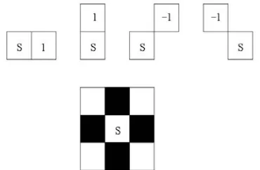
The simple second order neighborhood system N2 for two levels gray values and the control parameter θ1= θ2 = 1, θ3= θ4 = -1, without considering the

boundary, will generate a checkerboard texture, with size of every white and black. This can be explained as if we choose θ1= θ2 = 1, then pixels with opposite

gray values are favorable for the horizontal and vertical neighbors, and θ3= θ4 = -1, such that diagonal

neighbors tend to have similar gray values.

Figure 3. An illustration of cliques pair for N2 with the considering control parameters θ's to generate a checkerboard texture.

We modified the Ising model by changing the control parameters θ such that these parameters do not only depend on the pair of the clique types but also on the relative position of the site s in the clique. If, e.g., we consider N2 and the control parameter θ = (θ1,θ2 ,

θ3, θ4) as a vector, then the position of the θ 's is

shown in the Figures 4.

The generalized Ising potential function, can be written as

where the clique potential and the control parameter for every pair clique c of any shape is defined as in (6). T*(No) is the number clique. The control parameters θi

(s,t) may not only depend on the type of clique but, in general, also on the gray values xs,xt.

We know that the similarity or dissimilarity for a pixel to its neighborhood is measured by U(xs,xt) and low energy configurations are more likely than the higher one. Based on these two conditions, for synthesizing a binary images, θi (s,t) can be chosen as

but this implies that

)

Figure 4. Modified cliques pair for N2 with the considering control parameters θs

It gives the same probability for each image and that implies same probability for each gray scale value at each pixel!.

In Figure 5 we give an example for generating a binary image, i.e. a reference image. This image is initiated from the binary random image. We use modified cliques pair (Figure4) and Gibbs sampler with generalized Ising potential function (7). First, we train the initial image to get the parameters θi(s, t) as

the negative value of the potential function from the reference image. At first iteration, we get the left image of Figure5. After several iterations, the image gets better and better until it reaches the goal, i.e, the reference image, as it is depicted in Figure5 (right).

This modification is the first step for synthesizing the rich gray level texture. The complete approach can be seen in Halim [9].

Algorithm 1:

1. Calculate the gray level proportion of thenor-malized sample image.

2. Generate random image x with size K = k x nrow, M = l x ncol, k,l ∈ Z based on the gray level proportion which has calculated in Step 1.

3. Set TempConstant = L; InversTemp = log(2) / TempConstant; Set StopCriterion = 0.005 x K x; sweep = 1;

4. Use Metropolis sampler and Simulated annealing, Geman and Geman [8] synthesize the texture. repeat

set p = 1;

for i = KBound to (K - KBound) do for j = NBound to (M - MBound) do

(4)

JURNAL INFORMATIKA VOL. 8, NO. 2, NOPEMBER 2007: 115 - 118

118

5.2 Calculate the energy function Hold based on

(7)

5.3 Choose a new label uniformly random.

5.4 Calculate the energy function for the new composition Hnew based on (7).

5.5 if Hnew > Hold

p = exp(-InversTemp x (Hnew-Hold)

we replace the old label by the new one with probability p.

5.6 Recalculate the gray value proportion.

5.7 set Sweep = Sweep + 1; InversTemp = log (1+Sweep)/TempConstant.

until (StopCriterion is fulfilled) or (x satisfies stability criterion)

CONCLUTION AND REMARKS

The Ising model has properties that the potential for a clique with two different gray values is independent of the absolute difference of the gray values. This means that the Ising model could not make differences of more than two gray values. Therefore a further modification should be made for general gray images.

Figure 5. (left–right) Initial image, after some iterations and the final result

REFERENCES

1. C.O Acuna. “Texture modeling using Gibbs distributions”. CVGIP: Graphical Models and Image Processing, 54,3:210-222,1992.

2. J.E. Besag. “Spatial interaction and the statistical analysis of lattice system”. Journal of The Royal Statistical Society, series B, 36:192-326,1974

3. J.E. Besag. “On the statistical analysis of dirty pictures”. Journal of The Royal Statistical Society, series B, 48:259-302,1986.

4. A.A. Efros, and W.T. Freeman, “Image quilting for texture synthesis and transfer”. In E.Fiume, editor, Proceeding of SIGGRAPH 2001, Computer Graphics Proceedings, Annual Conferences Series, pages 341-346, ACM Press/ACM SIGGRAPH, August 2001

5. A.A. Efros and T.K. Leung, “ Texture synthesis by non-parametric sampling.” In IEEE International conference in Computer Vision, pages 1033-1038, Corfu, Greece, September 1999

6. D. Geman, “Random fields and inverse problem in imaging”. In P. Hennequin, editor, E’cole d’ E’te’ de Probabilite’ de Saint Flour XVIII, Lecture Notes in Mathematics, volume 1427, pages113-193. Springer Verlag, 1990.

7. S. Geman and D. Geman. „Stochastic relaxation, gibbs distribution, and the Bayesian restoration images. IEEE Transactions on Pattern Analysis and Machine Intelligence, 6:721-741, 1984

8. S. Geman and C. Graffigne. Markov random field image models and their applications, pages1496-1517, 1987

9. Halim, S, Spatially Adaptive detection of local disturbances in time series and stochastic pro-cessed in the lattice Z2. Ph.D dissertation, Technische Universtaet Kaiserslautern, 2005

10. R. D. Paget. Nonparametric Markov Random Field Models for Natural Texture Images. PhD thesis, The University of Queensland, Australia, 1999. http://www.vision.ee.ethz.ch/_rpaget/publi-cations.htm.

11. L. Y. Wie and M. Levoy. Fast texture synthesis using tree-structured vector quantization. In

SIGGRAPH, pages 479-488, 2000.