Clif ford Algebras and Possible Kinematics
Alan S. MCRAE
Department of Mathematics, Washington and Lee University, Lexington, VA 24450-0303, USA E-mail: [email protected]
Received April 30, 2007, in final form July 03, 2007; Published online July 19, 2007 Original article is available athttp://www.emis.de/journals/SIGMA/2007/079/
Abstract. We review Bacry and L´evy-Leblond’s work on possible kinematics as applied to 2-dimensional spacetimes, as well as the nine types of 2-dimensional Cayley–Klein geo-metries, illustrating how the Cayley–Klein geometries give homogeneous spacetimes for all but one of the kinematical groups. We then construct a two-parameter family of Clifford algebras that give a unified framework for representing both the Lie algebras as well as the kinematical groups, showing that these groups are true rotation groups. In addition we give conformal models for these spacetimes.
Key words: Cayley–Klein geometries; Clifford algebras; kinematics
2000 Mathematics Subject Classification: 11E88; 15A66; 53A17
As long as algebra and geometry have been separated, their progress have been slow and their uses limited; but when these two sciences have been united, they have lent each mutual forces, and have marched together towards perfection.
Joseph Louis Lagrange (1736–1813)
The first part of this paper is a review of Bacry and L´evy-Leblond’s description of possible kinematics and how such kinematical structures relate to the Cayley–Klein formalism. We review some of the work done by Ballesteros, Herranz, Ortega and Santander on homogeneous spaces, as this work gives a unified and detailed description of possible kinematics (save for static kinematics). The second part builds on this work by analyzing the corresponding kinematical models from other unified viewpoints, first through generalized complex matrix realizations and then through a two-parameter family of Clifford algebras. These parameters are the same as those given by Ballesteros et. al., and relate to the speed of light and the universe time radius.
Part I. A review of kinematics via Cayley–Klein geometries
1
Possible kinematics
As noted by Inonu and Wigner in their work [17] on contractions of groups and their repre-sentations, classical mechanics is a limiting case of relativistic mechanics, for both the Galilei group as well as its Lie algebra are limits of the Poincar´e group and its Lie algebra. Bacry and L´evy-Leblond [1] classified and investigated the nature of all possible Lie algebras for kinema-tical groups (these groups are assumed to be Lie groups as 4-dimensional spacetime is assumed to be continuous) given the three basic principles that
(i) space is isotropic and spacetime is homogeneous,
(ii) parity and time-reversal are automorphisms of the kinematical group, and
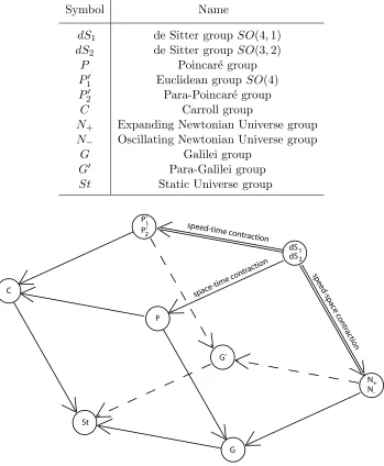
Table 1. The 11 possible kinematical groups.
Symbol Name
dS1 de Sitter group SO(4,1)
dS2 de Sitter group SO(3,2)
P Poincar´e group
P′
1 Euclidean groupSO(4)
P2′ Para-Poincar´e group
C Carroll group
N+ Expanding Newtonian Universe group
N− Oscillating Newtonian Universe group
G Galilei group
G′ Para-Galilei group
St Static Universe group
speed-time
contraction dS1 dS2
P’2 P’1
P
G’
G C
St
space-t ime co
ntracti on
sp ee
d-spac
e c ont
rac tion
N+
N
-Figure 1. The contractions of the kinematical groups.
The resulting possible Lie algebras give 11 possible kinematics, where each of the kinematical groups (see Table 1) is generated by its inertial transformations as well as its spacetime trans-lations and spatial rotations. These groups consist of the de Sitter groups and their rotation-invariant contractions: the physical nature of a contracted group is determined by the nature of the contraction itself, along with the nature of the parent de Sitter group. Below we will illustrate the nature of these contractions when we look more closely at the simpler case of a 2-dimensional spacetime. For Fig. 1, note that a “upper” face of the cube is transformed under one type of contraction into the opposite face.
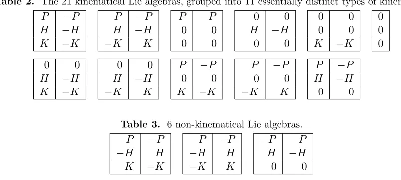
Table 2. The 21 kinematical Lie algebras, grouped into 11 essentially distinct types of kinematics.
P −P P −P P −P 0 0 0 0 0
H −H H −H 0 0 H −H 0 0 0
K −K −K K 0 0 0 0 K −K 0
0 0 0 0 P −P P −P P −P
H −H H −H 0 0 0 0 H −H
K −K −K K K −K −K K 0 0
Table 3. 6 non-kinematical Lie algebras.
P −P P −P −P P
−H H −H H H −H
K −K −K K 0 0
LetK denote the generator of the inertial transformations,H the generator of time transla-tions, andP the generator of space translations. As space is one-dimensional, space is isotropic. In the following section we will see how to construct, for each possible kinematical structure, a spacetime that is a homogeneous space for its kinematical group, so that basic principle (i) is satisfied.
Now let Π and Θ denote the respective operations of parity and time-reversal: K must be odd under both Π and Θ. Our basic principle (ii) requires that the Lie algebra is acted upon by theZ2⊗Z2 group of involutions generated by
Π : (K, H, P)→(−K, H,−P) and Θ : (K, H, P)→(−K,−H, P).
Finally, basic principle (iii) requires that the subgroup generated byK is noncompact, even though we will allow for the universe to be closed, or even for closed time-like worldlines to exist. We do not wish for e0K=eθK for some non-zeroθ, for then we would find it possible for a boost to be no boost at all!
As each Lie bracket [K, H], [K, P], and [H, P] is invariant under the involutions Π and Θ as well as the involution
Γ = ΠΘ : (K, H, P)→(K,−H,−P),
we must have that [K, H] =pP, [K, P] =hH, and [H, P] =kK for some constantsk,h, and p. Note that these Lie brackets are also invariant under the symmetries defined by
SP :{K↔H, p↔ −p, k↔h}, SH :{K ↔P, h↔ −h, k↔ −p}, and
SK :{H ↔P, k↔ −k, h↔p},
and that the Jacobi identity is automatically satisfied for any triple of elements of the Lie algebra.
We can normalize the constants k, h, and p by a scale change so that k, h, p ∈ {−1,0,1}, taking advantage of the simple form of the Lie brackets for the basis elements K, H, and P. There are then 33 possible Lie algebras, which we tabulate in Tables 2 and 3 with columns that have the following form:
Table 4. Some kinematical groups along with their notation and structure constants. Anti-de Sitter Oscillating Newtonian Universe Para-Minkowski Minkowski
adS N− M′ M
[K, H] P P 0 P
[K, P] H 0 H H
[H, P] K K K 0
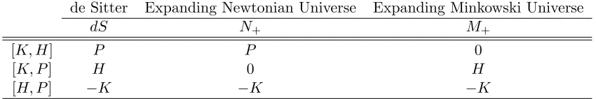
Table 5. Some kinematical groups along with their notation and structure constants.
de Sitter Expanding Newtonian Universe Expanding Minkowski Universe
dS N+ M+
[K, H] P P 0
[K, P] H 0 H
[H, P] −K −K −K
We also pair each Lie algebra with its image under the isomorphism given byP ↔ −P,H↔ −H,
K ↔ −K, and [⋆, ⋆⋆]↔[⋆⋆, ⋆], for both Lie algebras then give the same kinematics. There are then 11 essentially distinct kinematics, as illustrated in Table 2. Also (as we shall see in the next section) each of the other 6 Lie algebras (that are given in Table 3) violate the third basic principle, generating a compact group of inertial transformations.
These non-kinematical Lie algebras are the lie algebras for the motion groups for the elliptic, hyperbolic, and Euclidean planes: let us denote these respective groups as El,H, and Eu.
We name the kinematical groups (that are generated by the boosts and translations) in concert with the 4-dimensional case (see Tables 4, 5, and 6). Each of these kinematical groups is either the de Sitter or the anti-de Sitter group, or one of their contractions. We can contract with respect to any subgroup, giving us three fundamental types of contraction: space, speed-time, and space-time contractions, corresponding respectively to contracting to the subgroups generated by H,P, and K.
Speed-space contractions. We make the substitutions K → ǫK and P → ǫP into the Lie algebra and then calculate the singular limit of the Lie brackets as ǫ → 0. Physically the velocities are small when compared to the speed of light, and the spacelike intervals are small when compared to the timelike intervals. Geometrically we are describing spacetime near a timelike geodesic, as we are contracting to the subgroup that leaves this worldline invariant, and so are passing from relativistic to absolute time. So adS is contracted to N− while dS is contracted to N+, for example.
Speed-time contractions. We make the substitutions K → ǫK and H → ǫH into the Lie algebra and then calculate the singular limit of the Lie brackets as ǫ → 0. Physically the velocities are small when compared to the speed of light, and the timelike intervals are small when compared to the spacelike intervals. Geometrically we are describing spacetime near a spacelike geodesic, as we are contracting to the subgroup that leaves invariant this set of simultaneous events, and so are passing from relativistic to absolute space. Such a spacetime may be of limited physical interest, as we are only considering intervals connecting events that are not causally related.
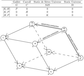
[image:4.612.101.526.189.260.2]Table 6. Some kinematical groups along with their notation and structure constants. Galilei Carroll Static de Sitter Universe Static Universe
G C SdS St
[K, H] P 0 0 0
[K, P] 0 H 0 0
[H, P] 0 0 K 0
speed-tim
e contraction
dS adS M+
M’
M
SdS
G C
St
space-t ime con
tractio n
sp eed
-sp ace
co ntr
ac tio
n
N+ N -1
2
3 4
5
6 7
8
Figure 2. The contractions of the kinematical groups for 2-dimensional spacetimes.
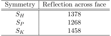
Fig. 2 illustrates several interesting relationships among the kinematical groups. For example, Table 7 gives important classes of kinematical groups, each class corresponding to a face of the figure, that transform to another class in the table under one of the symmetriesSH,SP, or SK, provided that certain exclusions are made as outlined in Table 8. The exclusions are necessary under the given symmetries as some kinematical algebras are taken to algebras that are not kinematical.
2
Cayley–Klein geometries
In this section we wish to review work done by Ballesteros, Herranz, Ortega and Santander on homogeneous spaces that are spacetimes for kinematical groups, and we begin with a bit of history concerning the discovery of non-Euclidean geometries. Franz Taurinus was the first to explicitly give mathematical details on how a hypothetical sphere of imaginary radius would have a non-Euclidean geometry, what he called log-spherical geometry, and this was done via hyperbolic trigonometry (see [5] or [18]). Felix Klein1 is usually given credit for being the first
to give a complete model of a non-Euclidean geometry2
: he built his model by suitably adapting
1
Roger Penrose [21] notes that it was Eugenio Beltrami who first discovered both the projective and conformal models of the hyperbolic plane.
2
Table 7. Important classes of kinematical groups and their geometrical configurations in Fig. 2. Class of groups Face
Relative-time 1247 Absolute-time 3568 Relative-space 1346 Absolute-space 2578 Cosmological 1235
Local 4678
Table 8. The 3 basic symmetries are represented by reflections of Fig. 2, with some exclusions. Symmetry Reflection across face
SH 1378 (excluding M+)
SP 1268 (excludingadS and N−)
SK 1458
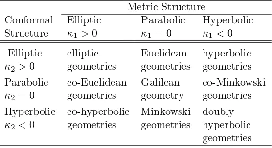
Arthur Cayley’s metric for the projective plane. Klein [19] (originally published in 1871) went on, in a systematic way, to describe nine types of two-dimensional geometries (what Yaglom [28] calls Cayley–Klein geometries) that were then further investigated by Sommerville [26]. Yaglom gave conformal models for these geometries, extending what had been done for both the projective and hyperbolic planes. Each type of geometry is homogeneous and can be determined by two real constants κ1 and κ2 (see Table 9). The names of the geometries when κ2 ≤0 are those as given by Yaglom, and it is these six geometries that can be interpreted as spacetime geometries. Following Taurinus, it is easiest to describe a bit of the geometrical nature of these geometries by applying the appropriate kind of trigonometry: we will see shortly how to actually construct a model for each geometry. Letκ be a real constant. The unit circlea2
+κb2
= 1 in the plane
R2 ={(a, b)}with metric ds2 =da2
+κdb2
can be used to defined the cosine
Cκ(φ) =
cos (√κ φ), ifκ >0,
1, ifκ= 0,
cosh √−κ φ
, ifκ <0,
and sine
Sκ(φ) =
1
√κsin (√κ φ), ifκ >0,
φ, ifκ= 0,
1 √
−κsinh √
−κ φ
, ifκ <0
functions: here (a, b) = (Cκ(φ), Sκ(φ)) is a point on the connected component of the unit circle containing the point (1,0), andφ is the signed distance from (1,0) to (a, b) along the circular
arc, defined modulo the length √2π
κ of the unit circle when κ >0. We can also write down the
power series for these analytic trigonometric functions:
Cκ(φ) = 1− 1 2!κφ
2 + 1
4!κ 2
φ4 +· · ·,
Sκ(φ) =φ− 1 3!κφ
3 + 1
5!κ 2
φ5
+· · ·.
Table 9. The 9 types of Cayley–Klein geometries. Metric Structure
Conformal Elliptic Parabolic Hyperbolic Structure κ1>0 κ1 = 0 κ1 <0
Elliptic elliptic Euclidean hyperbolic
κ2>0 geometries geometries geometries Parabolic co-Euclidean Galilean co-Minkowski
κ2= 0 geometries geometry geometries Hyperbolic co-hyperbolic Minkowski doubly
κ2<0 geometries geometries hyperbolic geometries
the unit circle consists of two parallel straight lines, and we will say that our trigonometry is parabolic. We can use such a trigonometry to define the angleφbetween two lines, and another independently chosen trigonometry to define the distance between two points (as the angle between two lines, where each line passes through one of the points as well as a distinguished point).
At this juncture it is not clear that such geometries, as they have just been described, are of either mathematical or physical interest. That mathematicians and physicists at the beginning of the 20th century were having similar thoughts is perhaps not surprising, and Walker [27] gives an interesting account of the mathematical and physical research into non-Euclidean geometries during this period in history. Klein found that there was a fundamental unity to these geometries, and so that alone made them worth studying. Before we return to physics, let us look at these geometries from a perspective that Klein would have appreciated, describing their motion groups in a unified manner.
Ballesteros, Herranz, Ortega and Santander have constructed the Cayley–Klein geometries as homogeneous spaces3 by looking at real representations of their motion groups. These motion
groups are denoted by SOκ1,κ2(3) (that we will refer to as the generalized SO(3) or simply by SO(3)) with their respective Lie algebras being denoted bysoκ1,κ2(3) (that we will refer to as the
generalizedso(3) or simply byso(3)), and most if not all of these groups are probably familiar to the reader (for example, if both κ1 and κ2 vanish, then SO(3) is the Heisenberg group). Later on in this paper we will use Clifford algebras to show how we can explicitly think of SO(3) as a rotation group, where each element of SO(3) has a well-defined axis of rotation and rotation angle.
Now a matrix representation ofso(3) is given by the matrices
H =
0 −κ1 0
1 0 0
0 0 0
, P =
0 0 −κ1κ2
0 0 0
1 0 0
, and K=
0 0 0
0 0 −κ2
0 1 0
,
where the structure constants are given by the commutators
[K, H] =P, [K, P] =−κ2H, and [H, P] =κ1K.
By normalizing the constants we obtain matrix representations of the adS, dS, N−, N+, M, andGLie algebras, as well as the Lie algebras for the elliptic, Euclidean, and hyperbolic motion groups, denoted El, Eu, and H respectively. We will see at the end of this section how the
3
Cayley–Klein spaces can also be used to give homogeneous spaces for M′, M+, C, and SdS
(but not for St). One benefit of not normalizing the parameters κ1 and κ2 is that we can easily obtain contractions by letting κ1→0 or κ2 →0.
Elements ofSO(3) are real-linear, orientation-preserving isometries of R3 ={(z, t, x))} im-bued with the (possibly indefinite or degenerate) metric ds2 = dz2 +κ
1dt2 +κ1κ2dx2. The one-parameter subgroupsH,P, andKgenerated respectively by H,P, andK consist of matri-ces of the form
eαH =
Cκ1(α) −κ1Sκ1(α) 0 Sκ1(α) Cκ1(α) 0
0 0 1
, eβP =
Cκ1κ2(β) 0 −κ1κ2Sκ1κ2(β)
0 1 0
Sκ1κ2(β) 0 Cκ1κ2(β)
,
and
eθK =
1 0 0
0 Cκ2(θ) −κ2Sκ2(θ)
0 Sκ2(θ) Cκ2(θ)
(note that the orientations induced on the coordinate planes may be different than expected). We can now see that in order forKto be non-compact, we must have thatκ2 ≤0, which explains the content of Table 3.
The spaces SO(3)/K, SO(3)/H, and SO(3)/P are homogeneous spaces for SO(3). When
SO(3) is a kinematical group, thenS ≡SO(3)/K can be identified with the manifold of space-time translations. Regardless of the values ofκ1andκ2however,S is the Cayley–Klein geometry with parameters κ1 and κ2, andS can be shown to have constant curvature κ1 (also, see [20]). So the angle between two lines passing through the origin (the point that is invariant under the subgroupK) is given by the parameter θ of the element ofK that rotates one line to the other (and so the measure of angles is related to the parameter κ2). Similarly if one point can be taken to another by an element ofHorP respectively, then the distance between the two points is given by the parameterαorβ, (and so the measure of distance is related to the parameterκ1 or toκ1κ2). Note that the spacesSO(3)/Hand SO(3)/P are respectively the spaces of timelike and spacelike geodesics for kinematical groups.
For our purposes we will also need to modelS as a projective geometry. First, we define the projective quadric ¯Σ as the set of points on the unit sphere Σ ≡ {(z, t, x) ∈ R3
|z2+κ 1t2 +
κ1κ2x2 = 1} that have been identified by the equivalence relation (z, t, x)∼(−z,−t,−x). The group SO(3) acts on ¯Σ, and the subgroup K is then the isotropy subgroup of the equivalence class O = [(1,0,0)]. The metricg on R3 induces a metric on ¯Σ that has κ
1 as a factor. If we then define the main metric g1 on ¯Σ by setting
ds2
1 = 1
κ1
ds2,
then the surface ¯Σ, along with its main metric (and subsidiary metric, see below), is a projective model for the Cayley–Klein geometry S. Note that in general g1 can be indefinite as well as nondegenerate.
The motion exp(θK) gives a rotation (or boost for a spacetime) of S, whereas the mo-tions exp(αH) and exp(βP) give translations ofS (time and space translations respectively for a spacetime). The parameters κ1 and κ2 are, for the spacetimes, identified with the universe time radius τ and speed of lightc by the formulae
κ1=± 1
τ2 and κ2 =−
1
dS
adS M
+ M’
M
SdS
G C
St
N+ N -1
2
3 4
5
6 7
8
El H
[image:9.612.135.487.57.290.2]Eu
Figure 3. The 9 kinematical and 3 non-kinematical groups.
Table 10. The 3 basic symmetries are given as reflections of Fig. 3.
Symmetry Reflection across face
SH 1378
SP 1268
SK 1458
For the absolute-time spacetimes with kinematical groups N−, G, and N+, where κ2 = 0 and c =∞, we foliate S so that each leaf consists of all points that are simultaneous with one another, and then SO(3) acts transitively on each leaf. We then define the subsidiary metricg2 along each leaf of the foliation by setting
ds2
2 = 1
κ2
ds2
1.
Of course whenκ26= 0, the subsidiary metric can be defined on all of ¯Σ. The groupSO(3) acts onS by isometries of g1, by isometries ofg2 whenκ2 6= 0 and, whenκ2= 0, on the leaves of the foliation by isometries ofg2.
It remains to be seen then how homogeneous spacetimes for the kinematical groupsM+, M′, C, and SdS may be obtained from the Cayley–Klein geometries. In Fig. 3 the face 1346 contains the motion groups for all nine types of Cayley–Klein geometries, and the symmetries SH,SP, and SK can be represented as symmetries of the cube, as indicated in Table 104. As vertices 1 and 8 are in each of the three planes of reflection, it is impossible to get St from any one of the Cayley–Klein groups through the symmetries SH, SP, and SK. Under the symmetry SK, respective spacetimes for M+, M′, and C are given by the spacetimes SO(3)/K for N+, N−, and G, where space and time translations are interchanged.
Under the symmetrySH, the spacetime forSdSis given by the homogeneous spaceSO(3)/P forG, as boosts and space translations are interchanged bySH. Note however that there actually
4
[image:9.612.223.403.357.416.2]are no spacelike geodesics for G, as the Cayley–Klein geometry S =SO(3)/K for κ1 =κ2 = 0 can be given simply by the plane R2 = {(t, x)} with ds2
= dt2
as its line element5
. Although
SO(3)/P is a homogeneous space for SO(3), SO(3) does not act effectively onSO(3)/P: since both [K, P] = 0 and [H, P] = 0, space translations do not act on SO(3)/P. Similarly, inertial transformations do not act on spacetime for SdS, or on Stfor that matter. Note thatSdS can be obtained from dS by P → ǫP, H → ǫH, and K → ǫ2
K, where ǫ → 0. So velocities are negligible even when compared to the reduced space and time translations.
In conclusion to Part I then, a study of all nine types of Cayley–Klein geometries affords us a beautiful and unified study of all 11 possible kinematics save one, the static kinematical structure. It was this study that motivated the author to investigate another unified approach to possible kinematics, save for that of the Static Universe.
Part II. Another unif ied approach to possible kinematics
3
The generalized Lie algebra
so
(3)
Preceding the work of Ballesteros, Herranz, Ortega, and Santander was the work of Sanjuan [23] on possible kinematics and the nine6
Cayley–Klein geometries. Sanjuan represents each kine-matical Lie algebra as a real matrix subalgebra of M(2,C), where C denotes the generalized complex numbers (a description of the generalized complex numbers is given below). This is accomplished using Yaglom’s analytic representation of each Caley–Klein geometry as a region ofC: for the hyperbolic plane this gives the well-known Poincar´e disk model. Sanjuan constructs the Lie algebra for the hyperbolic plane using the standard method, stating that this method can be used to obtain the other Lie algebras as well. Also, extensive work has been done by Gromov [6,7,8,9,10] on the generalized orthogonal groupsSO(3) (which we refer to simply as
SO(3)), deriving representations of the generalizedso(3) (which we refer to simply asso(3)) by utilizing the dual numbers as well as the standard complex numbers, where again it is tacitly assumed that the parameters κ1 and κ2 have been normalized. Also, Pimenov has given an axiomatic description of all Cayley–Klein spaces in arbitrary dimensions in his paper [22] via the dual numbers ik,k= 1,2, . . ., whereikim =imik6= 0 and i2k= 0.
Unless stated otherwise, we will not assume that the parameters κ1 and κ2 have been nor-malized, as we wish to obtain contractions by simply letting κ1 → 0 or κ2 → 0. Our goal in this section is to derive representations of so(3) as real subalgebras of M(2,C), and in the process give a conformal model ofS as a region of the generalized complex plane Calong with a hermitian metric, extending what has been done for the projective and hyperbolic planes7
. We feel that it is worthwhile to write down precisely how these representations are obtained in order that our later construction of a Clifford algebra is more meaningful.
The first step is to represent the generators of SO(3) by M¨obius transformations (that is, linear fractional transformations) of an appropriately defined region in the complex number plane C, where the points ofS are to be identified with this region.
Definition 1. By the complex number planeCκ we will mean{w=u+iv|(u, v)∈R2 andi2 = −κ} whereκ is a real-valued parameter.
Thus Cκ refers to the complex numbers, dual numbers, or double numbers when κ is nor-malized to 1, 0, or−1 respectively (see [28] and [12]). One may check thatCκ is an associative
5Yaglom writes in [28] about this geometry,
“. . . which, in spite of its relative simplicity, confronts the unini-tiated reader with many surprising results.”
6
Sanjuan and Yaglom both tacitly assume that both parametersκ1 andκ2 are normalized. 7
t
z
x Cκκ
1 2
Cκ
2
Cκ
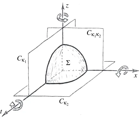
[image:11.612.200.427.56.251.2]1 Σ
Figure 4. The unit sphere Σ and the three complex planesCκ2,Cκ1, and Cκ1κ2.
algebra with a multiplicative unit, but that there are zero divisors when κ≤0. For example, if
κ= 0, then iis a zero-divisor. The reader will note below that 1
i appears in certain equations, but that these equations can always be rewritten without the appearance of any zero-divisors in a denominator. One can extendCκ so that terms like 1i are well-defined (see [28]). It is these zero divisors that play a crucial rule in determining the null-cone structure for those Cayley–Klein geometries that are spacetimes.
Definition 2. HenceforwardCwill denoteCκ2, as it is the parameterκ2 which determines the
conformal structure of the Cayley–Klein geometry S with parametersκ1 and κ2.
Theorem 1. The matrices 2iσ1, 2iσ2, and 21iσ3 are generators for the generalized Lie algebra
so(3), where so(3) is represented as a subalgebra of the real matrix algebra M(2,C), where
σ1=
1 0
0 −1
, σ2 =
0 1
κ1 0
and σ3 =
0 i
−κ1i 0
.
In fact, we will show that K, H, and P (the subgroups generated respectively by boosts, time and space translations) can be respectively represented by elements of SL(2,C) of the form eiθ2σ1, eiα2σ2, and e
β
2iσ3.
Note that whenκ1 = 1 andκ2 = 1, we recover the Pauli spin matrices, though my indexing is different, and there is a sign change as well: recall that the Pauli spin matrices are typically given as
σ1=
0 1 1 0
, σ2 =
0 −i
i 0
and σ3 =
1 0
0 −1
.
We will refer to σ1,σ2, and σ3 as given in the statement of Theorem 1 as the generalized Pauli spin matrices.
The remainder of this section is devoted to proving the above theorem. The reader may find Fig. 4 helpful. The respective subgroups K, H, and P preserve the z, x, and t axes as well as the Cκ2, Cκ1, and Cκ1κ2 number planes, acting on these planes as rotations. Also, as
these groups preserve the unit sphere Σ ={(z, t, x)|z2
are, respectively, circles of the form κ1ww¯ = 1 (there is no intersection when κ1 = 0 or when
κ1<0 andκ2 >0),ww¯ = 1, andww¯ = 1, wherew,w, andwdenote elements ofCκ2,Cκ1, and
Cκ1κ2 respectively. We will see in the next section how a general element of SO(3) behaves in
a manner similar to the generators of K,H, andP, utilizing the power of a Clifford algebra. So we will let the planez = 0 inR3 represent C(recall that Cdenotes Cκ2). We may then
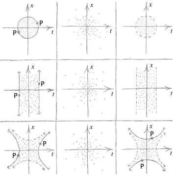
identify the points of S with a regionς of Cby centrally projecting Σ from the point (−1,0,0) onto the plane z= 0, projecting only those points (z, t, x)∈Σ with non-negative z-values. The regionς may be open or closed or neither, bounded or unbounded, depending on the geometry of S. Such a construction is well known for both the projective and hyperbolic planes RP2 and H2 and gives rise to the conformal models of these geometries. We will see later on how the conformal structure on Cagrees with that ofS, and then how the simple hermitian metric (see Appendix B)
ds2
= dwdw
1 +κ1|w| 22
gives the main metric g1 for S. This metric can be used to help indicate the general character of the region ς for each of the nine types of Cayley–Klein geometries, as illustrated in Fig. 5. Note that antipodal points on the boundary of ς (if there is a boundary) are to be identified. For absolute-time spacetimes (when κ2 = 0) the subsidiary metricg2 is given by
g2 =
dx2 1 +κ1t20
2
and is defined on lines w=t0 of simultaneous events. For all spacetimes, with Here-Now at the origin, the set of zero-divisors gives the null cone for that event.
Via this identification of points of S with points of ς, transformations of S correspond to transformations of ς. If the real parametersκ1 and κ2 are normalized to the valuesK1 and K2 so that
Ki =
1, ifκi>0, 0, ifκi= 0, −1, ifκi<0
then Yaglom [28] has shown that the linear isometries ofR3 (with metric ds2 =dz2+K 1dt2+
K1K2dx2) acting on ¯Σ project to those M¨obius transformations that preserve ς, and so these M¨obius transformations preserve cycles8
: a cycle is a curve of constant curvature, corresponding to the intersection of a plane in R3 with ¯Σ. We would like to show that elements of SO(3) project to M¨obius transformations if the parameters are not normalized, and then to find a realization of so(3) as a real subalgebra ofM(2,C).
Givenκ1 and κ2 we may define a linear isomorphism ofR3 as indicated below.
κ16= 0, κ2 6= 0 κ1 6= 0, κ2= 0 κ1 =κ2= 0
z7→z′ =z z7→z′ =z z7→z′ =z t7→t′ = √1
|κ1|
t t7→t′ = √1 |κ1|
t t7→t′ =t
x7→x′ = √ 1 |κ1κ2|
x x7→x′ =x x7→x′ =x
This transformation preserves the projection point (−1,0,0) as well as the complex planez= 0, and maps the projective quadric ¯Σ for parameters K1 and K2 to that for κ1 and κ2, and so
8
Yaglom projects from the point (z, t, x) = (−1,0,0) onto the planez= 1 whereas we project onto the plane
P
P
P
P
P
P
P
P
t
t
t
t
t
t
t
t
t
x
x
x
x
x
x
[image:13.612.136.491.56.417.2]x
x
x
Figure 5. The regionsς.
gives a correspondence between elements of SOK1,K2(3) with those ofSOκ1,κ2(3) as well as the
projections of these elements. As the M¨obius transformations of C are those transformations that preserve curves of the form
Im(w′1−w3′)(w′2−w′) (w′1−w′)(w2′ −w3)′
= 0
(where w′
1, w2′, andw′3 are three distinct points lying on the cycle), then if this form is invari-ant under the induced action of the linear isomorphism, then elements of SOκ1,κ2(3) project to
M¨obius transformations of ς. As a point (z, t, x) is projected to the point 0,z+1t , x z+1
corre-sponding to the complex number w = 1
z+1(t+Ix) ∈ CK2, if the linear transformation sends
(z, t, x) to (z′, t′, x′), then it sends w = 1
z+1(t+Ix) ∈ CK2 to w′ =
1
z′+1(t′ +ix′) ∈ Cκ2 = C,
where I2=
−K2 and i2 =−κ2. We can then write that
κ16= 0, κ2 6= 0 κ16= 0, κ2 = 0 κ1 =κ2 = 0
w= 1
z+1(t+Ix)7→ w= 1
z+1(t+Ix)7→ w= 1
z+1(t+Ix)7→
w′ = 1 z+1
1 √
|κ1|
t+√I |κ2|
x
w′ = 1 z+1
1 √
|κ1| t+Ix
And so
Im(w1−w3)(w2−w) (w1−w)(w2−w3)
= 0 ⇐⇒ Im(w′1−w′3)(w2′ −w′) (w′1−w′)(w′2−w′3)
= 0,
as can be checked directly, and we then have that elements of SO(3) project to M¨obius trans-formations ofς.
The rotations eθK preserve the complex number plane z = t+ix = 0 and so correspond simply to the transformations of C given by w 7→ eiθw, as eiθ = C
κ2(θ) +iSκ2(θ), keeping in
mind that i2
=−κ2. Now in order to express this rotation as a M¨obius transformation, we can write
w7→ e
θ
2iw+ 0
0w+e−θ2i .
Since there is a group homomorphism from the subgroup of M¨obius transformations correspon-ding to SO(3) to the group M(2,C) of 2×2 matrices with entries in C, this transformation being defined by
aw+b cw+d 7→
a b c d
,
each M¨obius transformation is covered by two elements of SL(2,C). So the rotations eθK
correspond to the matrices
± e θ
2i 0
0 e−θ2i !
=±e
θ
2i
1 0
0 −1
.
For future reference let us now define
σ1≡
1 0
0 −1
,
where i
2σ1 is then an element of the Lie algebra so(3).
We now wish to see which elements of SL(2,C) correspond to the motions eαH and eβP. The x-axis, the zt-coordinate plane, and the unit sphere Σ, are all preserved by eαH. So the
zt-coordinate plane is given the complex structure Cκ1 = {w = z +it|i
2
= −κ1}, for then the unit circle ww = 1 gives the intersection of Σ with Cκ1, and the transformation induced
on Cκ1 by e
αH is simply given by
w 7→ eiαw. Similarly the transformation induced by eβP on Cκ1κ2 ={w=z+ix|i
2
=−κ1κ2}is given by w7→eiβw.
In order to explicitly determine the projection of the rotation w 7→ eiαw of the unit circle inCκ1 and also that of the rotationw7→e
iβwof the unit circle inC
κ1κ2, note that the projection
point (z, t, x) = (−1,0,0) lies in either unit circle and that projection sends a point on the unit circle (save for the projection point itself) to a point on the imaginary axis as follows:
w=eiφ7→iTκ1
φ
2
, w=eiφ7→iTκ
1κ2
φ
2
(where Tκ is the tangent function) for
Tκ
µ
2
= Sκ(µ)
Cκ(µ) + 1
noting that a pointa+ibon the unit circlewwof the complex planeCκcan be written asa+ib=
eiψ=C
κ(ψ) +iSκ(ψ). So the rotationseαH and eβP induce the respective transformations
iTκ1
φ
2
7→iTκ1
φ+α
2
, iTκ1κ2
φ
2
7→iTκ1κ2
φ+β
2
on the imaginary axes. We know that such transformations of either imaginary or real axes can be extended to M¨obius transformations, and in fact uniquely determine such M¨obius maps. For example, if w=iTκ1
φ 2
, then we have that
w7→ w +iTκ1
α 2
1−κ1w i Tκ1
α 2
or
w7→ Cκ1
α 2
w+iSκ1
α 2
−κ1
i Sκ1
α 2
w+Cκ1
α 2
with corresponding matrix representation
± Cκ1
α 2
iSκ1
α 2
iSκ1
α 2
Cκ1
α 2
!
inSL(2, Cκ1), where we have applied the trigonometric identity 9
Tκ(µ±ψ) =
Tκ(µ)±Tκ(ψ) 1∓κTκ(µ)Tκ(ψ)
.
However, it is not these M¨obius transformations that we are after, but those corresponding transformations of C.
Now a transformation of the imaginary axis (thex-axis) of Cκ1κ2 corresponds to a
transfor-mation of the imaginary axis ofC(also thex-axis) while a transformation of the imaginary axis of Cκ1 (the t-axis) corresponds to a transformation of the real axis of C (also thet-axis). For
this reason, values on thex-axis, which are imaginary for both theCκ1κ2 as well as theCplane,
correspond as
iTκ1κ2
φ
2
=i√1 κ1
Tκ2 √κ 1 φ 2
ifκ1>0,
iTκ1κ2
φ
2
=i√1
−κ1
T−κ2
√ −κ1
φ
2
ifκ1<0, and
iTκ1κ2 φ 2 =i φ 2
ifκ1 = 0, as can be seen by examining the power series representation forTκ. The situation for the rotationeiα is similar. We can then compute the elements ofSL(2,C) corresponding toeαH and eβP as given in tables 13 and 14 in Appendix C. In all cases we have the simple result that those elements of SL(2,C) corresponding to eαH can be written as e2αiσ3 and those for eβP as
eiβ2σ2, where
σ2≡
0 1
κ1 0
and σ3 ≡
0 i
−κ1i 0
.
Thus 2iσ1, 2iσ2, and 1
2iσ3 are generators for the generalized Lie algebra so(3), a subalgebra of the real matrix algebra M(2,C).
9
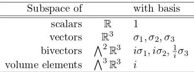
Table 11. The basis elements forCl3.
Subspace of with basis
scalars R 1
vectors R3 σ1, σ2, σ3 bivectors V2
R3 iσ1, iσ2,1iσ3 volume elements V3
R3
i
4
The Clif ford algebra
Cl
3Definition 3. LetCl3 be the 8-dimensional real Clifford algebra that is identified withM(2,C) as indicated by Table 11, where C denotes the generalized complex numbers Cκ2. Here we
identify the scalar 1 with the identity matrix and the volume element i with the 2×2 identity matrix multiplied by the complex scalari: in this case 1
iσ3 can be thought of as the 2×2 matrix
0 1
−κ1 0
. We will also identify the generalized Paul spin matrices σ1, σ2, and σ3 with the
vectors ˆi=h1,0,0i, ˆj=h0,1,0i, and ˆk=h0,0,1irespectively of the vector spaceR3 =
{(z, t, x)} given the Cayley–Klein inner product10
.
Proposition 1. Let Cl3 be the Clifford algebra given by Definition3. (i) The Clifford product σ2
i gives the square of the length of the vector σi under the Cayley– Klein inner product.
(ii) The center Cen(Cl3) of Cl3 is given by R⊕
V3
R3, the subspace of scalars and volume elements.
(iii) The generalized Lie algebra so(3) is isomorphic to the space of bivectors V2
R3, where
H = 1
2iσ3, P = i
2σ2, and K =
i
2σ1.
(iv) If nˆ = hn1
, n2
, n3
i and ~σ = hiσ1, iσ2, σ3/ii, then we will let ˆn·~σ denote the bivector
n1
iσ1+n2iσ2+n3 1iσ3. This bivector is simple, and the parallel vectorsinˆ·~σ and 1inˆ·~σ are perpendicular to any plane element represented bynˆ·~σ. Let η denote the line through the origin that is determined by inˆ·~σ or 1inˆ·~σ.
(v) The generalized Lie group SO(3) is also represented within Cl3, for if a is the vector
a1σ
1+a2σ2+a3σ3, then the linear transformation ofR3defined by the inner automorphism
a7→e−φ2nˆ·~σa e
φ
2nˆ·~σ
faithfully represents an element ofSO(3)as it preserves vector lengths given by the Cayley– Klein inner product, and is in fact a rotation, rotating the vectorha1
, a2
, a3
i about the axis
η through the angleφ. In this way we see that the spin group is generated by the elements
eθ2iσ1, e
β
2iσ2, and e
α
2iσ3.
(vi) Bivectors nˆ·~σ act as imaginary units as well as generators of rotations in the oriented planes they represent. Let κ be the scalar −(ˆn·~σ)2. Then if a lies in an oriented plane determined by the bivector nˆ·~σ, where this plane is given the complex structure of Cκ, then e−φ2nˆ·~σae
φ
2nˆ·~σ is simply the vector ha1, a2, a3i rotated by the angle φ in the complex
plane Cκ, where ι2
=−κ. So this rotation is given by unit complex multiplication.
10
The goal of this section is to prove Proposition 1. We can easily compute the following:
σ12= 1, σ22 =κ1, σ32 =κ1κ2,
σ3σ2 =−σ2σ3 =κ1iσ1, σ1σ3=−σ3σ1 =iσ2,
σ1σ2 =−σ2σ1 = 1
iσ3, σ1σ2σ3=−κ1i.
Recalling thatR3is given the Cayley–Klein inner product, we see thatσ2
i gives the square of the length of the vector σi. Note that when κ1 = 0, Cl3 is not generated by the vectors. Cen(Cl3) of Cl3 is given by R⊕V
3
R3, and we can check directly that if
H ≡ 1
2iσ3, P ≡ i
2σ2, and K≡
i
2σ1,
then we have the following commutators:
[H, P] =HP −P H = 1
4(σ3σ2−σ2σ3) =
κ1iσ1
2 =κ1K,
[K, H] =KH−HK = 1
4(σ1σ3−σ3σ1) =
iσ2 2 =P,
[K, P] =KP −P K = i 2
4 (σ1σ2−σ2σ1) =
iσ3
2 =−κ2H.
So the Lie algebra so(3) is isomorphic to the space of bivectorsV2
R3. The product of two vectors a= a1
σ1+a2σ2+a3σ3 and b= b1σ1+b2σ2+b3σ3 in Cl3 can be expressed as ab = a·b+a∧b = 1
2(ab+ba) + 1
2(ab−ba), where a·b = 1
2(ab+ba) =
a1b1+κ
1a2b2+κ1κ2a3b3 is the Cayley–Klein inner product and the wedge product is given by
a∧b= 1
2(ab−ba) =
−κ1iσ1 −iσ2 1iσ3
a1
a2
a3
b1 b2 b3
,
so that abis the sum of a scalar and a bivector: here|⋆|denotes the usual 3×3 determinant. By the properties of the determinant, ife∧f =g∧h and κ1 6= 0, then the vectors e and f span the same oriented plane as the vectorsgandh. Whenκ1 = 0 the bivector ˆn·~σis no longer simple in the usual way. For example, for the Galilean kinematical group (aka the Heisenberg group) where κ1 = 0 andκ2 = 0, we have that bothσ1∧σ3 =iσ2 and (σ1+σ2)∧σ3 =iσ2, so that the bivector iσ2 represents plane elements that do no all lie in the same plane11. Recalling that σ1, σ2, and σ3 correspond to the vectors ˆi, ˆj, and ˆk respectively, we observe that the subgroup P of the Galilean group fixes the t-axis and preserves both of these planes, inducing the same kind of rotation upon each of them: for the plane spanned by ˆiand ˆkwe have that
eβP :
ˆ
i
ˆ
k
7→
ˆ
i+βkˆ
ˆ
k
while for the plane spanned by ˆi+ ˆj and ˆkwe have that
eβP :
ˆ
i+ ˆj
ˆ
k
7→
ˆ
i+ ˆj+βˆk
ˆ
k
.
11
If we give either plane the complex structure of the dual numbers so that i2
= 0, then the rotation is given by simply multiplying vectors in the plane by the unit complex number eβi. We will see below that this kind of construction holds generally.
What we need for our construction below is that any bivector can be meaningfully expressed ase∧f for some vectors eand f, so that the bivector represents at least one plane element: we will discuss the meaning of the magnitude and orientation of the plane element at the end of the section. If the bivector represents multiple plane elements spanning distinct planes, so much the better. If ˆn=hn1
, n2
, n3
i and~σ=hiσ1, iσ2, σ3/ii, then we will let ˆn·~σdenote the bivector
B =n1
iσ1+n2iσ2+n3 1iσ3. Now if
a=n1σ3+κ1n 3
σ1, b=−n 1
σ2+κ1n 2
σ1, c=n 3
σ2+n 2
σ3,
then
a∧c=κ1n3nˆ·~σ, b∧a=κ1n1nˆ·~σ, b∧c=κ1n2nˆ·~σ,
where at least one of the bivectorsninˆ·~σ is non-zero as ˆn·~σ is non-zero. Ifκ
1 = 0 andn1 = 0, thenσ1∧c= ˆn·~σ. However, if bothκ1 = 0 andn16= 0, then it is impossible to havee∧f = ˆn·~σ: in this context we may simply replace the expression ˆn·~σ with the expressionσ3∧σ2 whenever
κ1 = 0 andn1 6= 0 (as we will see at the end of this section, we could just as well replace ˆn·~σ with any non-zero multiple ofσ3∧σ2). The justification for this is given by lettingκ1 →0, for then
e∧f = p|κ1|n2σ1−
n1
p
|κ1|
σ2
!
∧ p|κ1|
n3
n1σ1+ 1
p
|κ1|
σ3
!
= ˆn·~σ
shows that the plane spanned by the vectors e and f tends to the xt-coordinate plane. We will see below how each bivector ˆn·~σ corresponds to an element of SO(3) that preserves any oriented plane corresponding to ˆn·~σ: in the case whereκ1 = 0 and n1 6= 0, we will then have that this element preserves the tx-coordinate plane, which is all that we require.
It is interesting to note that the parallel vectors i(a∧b) and 1
i(a∧b) (when defined) are perpendicular to bothaandbwith respect to the Cayley–Klein inner product, as can be checked directly. However, due to the possible degeneracy of the Cayley–Klein inner product, there may not be a unique direction that is perpendicular to any given plane. The vector inˆ·~σ = −κ2n1σ1−κ2n2σ2+n3σ1 is non-zero and perpendicular to any plane element corresponding to ˆ
n·~σ except when both κ2 = 0 and n3 = 0, in which case inˆ·~σ is the zero vector. In this last case the vector 1iˆn·~σ=n1
σ1+n2σ2 gives a non-zero normal vector. In either case, let ηdenote the axis through the origin that contains either of these normal vectors.
Before we continue, let us reexamine those elements of SO(3) that generate the subgroups K,P, andH. Here the respective axes of rotation (parallel toσ1,σ2, andσ3) for the generators
eθK, eβP, and eαH are given by η, where ˆn·~σ is given by iσ
1 (or σ3 ∧σ2 by convention),
iσ2 = σ1 ∧σ3, and 1iσ3 = σ1 ∧σ2. These plane elements are preserved under the respective rotations. In fact, for each of these planes the rotations are given simply by multiplication by a unit complex number, as the zt-coordinate plane is identified with Cκ1, the zx-coordinate
plane with Cκ1κ2, and the tx-coordinate plane with Cκ2 as indicated in Fig. 4. Note that the
basis bivectors act as imaginary units in Cl3 since
1
iσ3 2
=−κ1, (iσ2) 2
=−κ1κ2, and (iσ1) 2
=−κ2.
The product of a vector a and a bivector B can be written as aB = a ⊣ B +a∧B = 1
2(aB−Ba) + 1
by B) and a volume elementa∧B. Let B=b∧cfor some vectors band c. Then
2a⊣(b∧c) =a(b∧c)−(b∧c)a= 1
2a(bc−cb)− 1
2(bc−cb)a
so that
4a⊣(b∧c) =cba+abc−acb−bca
=c(b·a+b∧a) + (a·b+a∧b)c−(a·c+a∧c)b−b(c·a+c∧a) = 2(b·a)c−2(c·a)b+c(b∧a) + (a∧b)c−(a∧c)b−b(c∧a) = 2(b·a)c−2(c·a)b+c(b∧a)−(b∧a)c+b(a∧c)−(a∧c)b
= 2(b·a)c−2(c·a)b+ 2 [c⊣(b∧a) +b⊣(a∧c)] = 2(b·a)c−2(c·a)b−2a⊣(c∧b)
= 2(b·a)c−2(c·a)b+ 2a⊣(b∧c)
where we have used the Jacobi identity
c⊣(b∧a) +b⊣(a∧c) +a⊣(c∧b) = 0,
recalling that M(2,C) is a matrix algebra where the commutator is given by left contraction. Thus
2a⊣(b∧c) = 2(b·a)c−2(c·a)b
and so
a⊣(b∧c) = (a·b)c−(a·c)b.
So the vector a ⊣ B lies in the plane determined by the plane element b ∧c. Because of the possible degeneracy of the Cayley–Klein metric, it is possible for a non-zero vector b that
b⊣(b∧c) = 0.
We will show that ifais the vectora1σ
1+a2σ2+a3σ3, then the linear transformation ofR3 defined by
a7→e−φ2nˆ·~σa e
φ
2nˆ·~σ
faithfully represents an element of SO(3) (and all elements are thus represented). In this way we see that the spin group is generated by the elements
eθ2iσ1, e
β
2iσ2, and e
α
2iσ3.
First, let us see how, using this construction, the vectors σ1, σ2, and σ3 (and hence the bivectorsiσ1,iσ2, and 1
iσ3) correspond to rotations of the coordinate axes (and hence coordinate planes) given by eθK,eβP, and eαH respectively. Since
eθ2iσ1 =Cκ 2
θ
2
+iSκ2
θ
2
σ1, e β
2iσ2 =Cκ
1κ2
β
2
+iSκ1κ2
β
2
σ2,
e2αiσ3 =Cκ
1
α
2
+1
iSκ1
α
2
σ3
and
2Cκ
φ
2
Sκ
φ
2
=Sκ(φ), Cκ2
φ
2
−κSκ2
φ
2
Cκ2
φ
2
+κSκ2
φ
2
= 1
(noting that Cκ is an even function whileSκ is odd) it follows that
e−θ2iσ1σje
θ
2iσ1 =
σ1 ifj= 1,
Cκ2(θ)σ2−Sκ2(θ)σ3 ifj= 2, Cκ2(θ)σ3+κ2Sκ2(θ)σ2 ifj= 3,
e−β2iσ2σje
β
2iσ2 =
Cκ1κ2(β)σ1+Sκ1κ2(β)σ3 ifj= 1,
σ2 ifj= 2,
Cκ1κ2(β)σ3−κ1κ2Sκ1κ2(β)σ1 ifj= 3,
e−2αiσ3σje α
2iσ3 =
Cκ1(α)σ1+Sκ1(α)σ2 ifj= 1, Cκ1(α)σ2−κ1Sκ1(α)σ1 ifj= 2,
σ3 ifj= 3.
So for each plane element, theσj transform as the components of a vector under rotation in the clockwise direction, given the orientations of the respective plane elements:
iσ1 is represented byσ3∧σ2, iσ2 =σ1∧σ3, and 1
iσ3 =σ1∧σ2.
Now we can write
eφ2nˆ·~σ = 1 +φ
2nˆ·~σ+ 1 2! φ 2 2
(ˆn·~σ)2+ 1 3!
φ
2
3
(ˆn·~σ)3+· · · .
If κ is the scalar−(ˆn·~σ)2, then
eφ2nˆ·~σ = 1− 1
2!
φ
2
2 κ+ 1
4!
φ
2
4
κ2− · · · !
+ ˆn·~σ φ
2 − 1 3! φ 2 3 κ+ 1
5!
φ
2
5
κ2− · · · !
=Cκ
φ
2
+ ˆn·~σSκ
φ
2
.
Asa=a1
σ1+a2σ2+a3σ3 is a vector, we can compute its length easily using Clifford multi-plication asaa= (a1
)2
+κ1(a2 )2
+κ1κ2(a3)2=|a|2. We would like to show thate− φ
2nˆ·~σae
φ
2nˆ·~σ is
also a vector with the same length asa. Ifg andh are elements of a matrix Lie algebra, then so ise−φadgh=e−φgheφg(see [25] for example). So ifB is a bivectorB1iσ
1+B2iσ2+B3 1iσ3, then
e−φ2nˆ·~σBe
φ
2ˆn·~σ is also a bivector. It follows thate−
φ
2nˆ·~σae
φ
2nˆ·~σ is a vector as the volume elementi
lies in Cen(Cl3) so thate−φ2nˆ·~σσ1e
φ
2nˆ·~σ,e−
φ
2nˆ·~σσ2e
φ
2nˆ·~σ, ande−
φ
2ˆn·~σσ3e
φ
2ˆn·~σ are all vectors. Since
e−φ2ˆn·~σae
φ
2nˆ·~σ e−
φ
2ˆn·~σae
φ
2ˆn·~σ
=e−φ2ˆn·~σ|a|2e
φ
2nˆ·~σ =|a|2e−
φ
2nˆ·~σe
φ
2ˆn·~σ =|a|2
it follows that e−φ2nˆ·~σae
φ
2ˆn·~σ has the same length as a. So the inner automorphism of R3 given
by a7→e−φ2nˆ·~σae
φ
2nˆ·~σ corresponds to an element ofSO(3). We will see in the next section that
Finally, note that e−φ2nˆ·~σ(ˆn·~σ)e
φ
2nˆ·~σ = ˆn·~σ as ˆn·~σ commutes with e
φ
2nˆ·~σ: so any plane
element represented by ˆn·~σ is preserved by the corresponding element of SO(3). In fact, if ˆ
n·~σ=a∧b for some vectors aand band κ is the scalar−(a∧b)2, then
e−φ2a∧b(a)e
φ
2a∧b=
Cκ φ 2
−(a∧b)Sκ
φ
2
(a)
Cκ φ 2
+ (a∧b)Sκ
φ
2
=C2
κ
φ
2
a+Cκ φ 2 Sκ φ 2
(a∧b)a(a∧b)
−Cκ φ 2 Sκ φ 2
(a∧b)a−Sκ2
φ
2
a(a∧b).
Since a(a∧b) =−(a∧b)a, then
e−φ2a∧b(a)e
φ
2a∧b= [C
κ(φ)−(a∧b)Sκ(φ)]a,
and so vectors lying in the plane determined by a∧b are simply rotated by an angle −φ, and this rotation is given by simple multiplication by a unit complex number e−iφ where i2
=−κ. Thus, the linear combination ua+vb is sent to ue−iφa+ve−iφb, and so the plane spanned by the vectors aand bis preserved.
The significance is that ifalies in an oriented plane determined by the bivector ˆn·~σ where this plane is given the complex structure ofCκ, thene−φ2nˆ·~σae
φ
2nˆ·~σ is simply the vectorarotated
by an angle of−φin the complex planeCκ, whereι2
=−κ. Furthermore, the axis of rotation is given byηasηis preserved (recall thatilies in the center ofCl3). Since the covariant components
σi ofaare rotated clockwise, the contravariant componentsaj are rotated counterclockwise. So ha1
, a2
, a3
i is rotated by the angle φin the complex planeCκ determined by ˆn·~σ.
If we useb∧a instead of a∧b to represent the plane element, then κ remains unchanged. Note however that, if cis a vector lying in this plane, then
e−φ2b∧ace−
φ
2b∧a= [C
κ(φ)−(b∧a)Sκ(φ)]c= [Cκ(−φ)−(a∧b)Sκ(−φ)]c
so that rotation by an angle ofφin the plane oriented according tob∧acorresponds to a rotation of angle −φ in the same plane under the opposite orientation as given bya∧b.
It would be appropriate at this point to note two things: one, the magnitude of ˆn·~σappears to be important, since κ = −(ˆn·~σ)2, and two, the normalization (n1
)2 + (n2
)2 + (n3
)2 = 1 of ˆn is somewhat arbitrary12
. These two matters are one and the same. We have chosen this normalization because it is a simple and natural choice. This particular normalization is not essential, however. For suppose that κ=−(a∧b)2
whileκ′=−(na∧b)2
, wherenis a positive constant. Let Cκ = {t+ix|i2
= −κ} with angle measure φ and Cκ′ = {t+ιx|ι2 = −κ′ =
−n2
κ} with angle measure θ: without loss of generality let κ>0. Then φ=nθ, for
eiθ = cos√κ′θ−√ι
κ′sin
√
κ′θ= cos n√κθ
−n√ι
κsin n
√
κθ
= cos √κφ
−√i
κsin
√
κφ
=eiφ.
So we see thatSO(3) is truly a rotation group, where each element has a distinct axis of rotation as well as a well-defined rotation angle.
12
Due to dimension requirements some kind of normalization is needed as we cannot haveφ,n1 ,n2
5
SU
(2)
Since the generators of the generalized Lie group SO(3) can be represented by inner automor-phisms of the subspace R3 of vectors of Cl
3 (see Definition 3), then every element of SO(3) can be represented by an inner automorphism, as the composition of inner automorphisms is an inner automorphism. On the other hand, we’ve seen that any inner automorphism represents an element ofSO(3). In fact, each rotation belonging toSO(3) is then represented by two elements ±eφ2nˆ·~σ of SL(2,C), where as usual C denotes the generalized complex number Cκ
2: we will
denote the subgroup of SL(2,C) consisting of elements of the form±eφ2ˆn·~σ by SU(2).
Definition 4. Let Abe the matrix
A=
κ1 0
0 1
.
We will now use Definition 4 to show thatSU(2) is a subgroup of the subgroupGofSL(2,C) consisting of those matrices U whereU⋆AU =A: in fact, both these subgroups of SL(2,C) are one and the same, as we shall see. Now
eφ2ˆn·~σ⋆Ae
φ
2nˆ·~σ = Cκ φ 2
+ (ˆn·~σ)⋆Sκ φ 2 A Cκ φ 2
+ ˆn·~σSκ
φ
2
=C2
κ
φ
2
A+ (ˆn·~σ)⋆A(ˆn·~σ)S2
κ
φ
2
+A(ˆn·~σ)Cκ φ 2 Sκ φ 2
+ (ˆn·~σ)⋆ACκ φ 2 Sκ φ 2 =A
because A(ˆn·~σ) =−(ˆn·~σ)⋆Aimplies that
A(ˆn·~σ)Cκ φ 2 Sκ φ 2
+ (ˆn·~σ)⋆ACκ φ 2 Sκ φ 2 = 0
and (ˆn·~σ)⋆A(ˆn·~σ) =−A(ˆn·~σ)2 =κA implies that
C2 κ φ 2
A+ (ˆn·~σ)⋆A(ˆn·~σ)S2
κ
φ
2
=C2
κ
φ
2
A+κS2
κ
φ
2
A=A.
So SU(2) is a subgroup of the subgroup G of SL(2,C) consisting of those matrices U where
U⋆AU =A.
We can characterize this subgroupG as
α β
−κ1β α
|α, β ∈Candαα+κ1ββ = 1
.
Now
eφ2nˆ·~σ = C2 κ φ 2
+n1iS2
κ
φ 2
n2iS2
κ
φ 2
+n3S2
κ φ 2 n2
κ1iSκ2
φ 2
−n3
κ1Sκ2
φ 2 C2 κ φ 2
−n1
iS2 κ φ 2
as can be checked directly, recalling that
eφ2nˆ·~σ =C κ
φ
2
+ (ˆn·~σ)Sκ
φ
2
where
κ=−(ˆn·~σ)2 = n12
κ2+ n2
2
κ1κ2+ n3
2 κ1.
Thus deteφ2nˆ·~σ
= 1, and we see that any element of Gcan be written in the form eφ2ˆn·~σ. So
the group SU(2) can be characterized by
SU(2) =
α β
−κ1β α
|α, β ∈Candαα+κ1ββ = 1
.
Note that ifU(λ) is a curve passing through the identity at λ= 0, then
d dλ
λ=0
(U⋆AU =A) =⇒ U˙⋆A+AU˙ = 0
so that su(2) consists of those elements B of M(2,C) such that B⋆A+AB = 0. Although
SU(2) is a double cover of SO(3), it is not necessarily the universal cover for SO(3), nor even connected, for sometimesSO(3) is itself simply-connected. Thus we have shown that:
Theorem 2. The Clifford algebra Cl3 can be used to construct a double cover of the generalized Lie group SO(3), for a vectora can be rotated by the inner automorphism
R3 →R3, a7→s−1as where s is an element of the group
Spin(3) =
α β
−κ1β α
|α, β∈Candαα+κ1ββ = 1
,
where C denotes the generalized complex number Cκ2.
Lemma 1. We define the generalized special unitary group SU(2) to be Spin(3). Then su(2) consists of those matrices B of M(2,C) such that B⋆A+AB= 0.
6
The conformal completion of
S
Yaglom [28] has shown how the complex plane Cκ may be extended to a Riemann sphere Γ or inversive plane13
(and so dividing by zero-divisors is allowed), upon which the entire set of M¨obius transformations acts globally and so gives a group of conformal transformations. In this last section we would like to take advantage of the simple structure of this conformal group and give the conformal completion of S, where S is conformally embedded simply by inclusion of the regionς lying inC and therefore lying in Γ. Herranz and Santander [16] found a conformal completion of S by realizing the conformal group as a group of linear transformations acting on R4
, and then constructing the conformal completion as a homogeneous phase space of this conformal group. The original Cayley–Klein geometry S was then embedded into its confor-mal completion by one of two methods, one a group-theoretical one involving one-parameter subgroups and the other stereographic projection.
The 6-dimensional real Lie algebra for SL(2,C) consist of those matrices in M(2,C) with trace equal to zero. In addition to the three generators H,P, and K
H = 1
2iσ3=
0 1
2 −κ1
2 0
, P = i
2σ2 =
0 2i κ1i
2 0
, K = i
2σ1 =
i
2 0
0 −2i
13
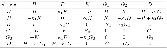
Table 12. Additional basis elements forsl(2,C).
⋆⋆ ⋆ H P K G1 G2 D
H 0 κ1K −P D K −H−κ1G1
P −κ1K 0 κ2H K −κ2D −P+κ1G2
K P −κ2H 0 −S2 κ2G2 0
G1 −D −K S2 0 0 G1
G2 −K κ2D −κ2G2 0 0 G2
D H+κ1G1 P−κ1G2 0 −G1 −G2 0
that come from the generalized Lie groupSO(3) of isometries ofS, we have three other generators forSL(2,C): one, labeledD, for the subgroup of dilations centered at the origin and two others, labeled G1 and G2, for “translations”. It is these transformations D, G1,G2, that necessitate extendingς to the entire Riemann sphere Γ, upon which the set of M¨obius transformations acts as a conformal group. Note that the following correspondences for the M¨obius transformations
w7→ w+t and w7→ w+ti (for real parametert) are valid only if κ1 6= 0, which explains why our “translations” G1 and G2 are not actually translations:
exp
t
0 1 0 0
=
1 t
0 1
⇄ w7→w+t,
exp
t
0 i
0 0
=
1 ti
0 1
⇄ w7→w+ti.
Please see Tables 15 and 16. The structure constants [⋆, ⋆⋆] for this basis of sl(2,C) (which is the same basis as that given in [15] save for a sign change in G2) are given by Table 12.
A
Appendix: Trigonometric identities
The following trigonometric identities are taken from [14] and [15], and are used throughout Sections 3, 4, and 5
d
dφCκ(φ) =−κSκ(φ), d
dφSκ(φ) =Cκ(φ),
d dφT
−1 κ (φ) =
1 1 +κφ2,
C2
κ(φ) +κS 2
κ(φ) = 1, Cκ(2φ) =Cκ2(φ)−κS 2
κ(φ), Sκ(2φ) = 2Cκ(φ)Sκ(φ),
Tκ
φ
2
= Sκ(φ)
Cκ(φ) + 1
, Tκ(φ±ψ) =
Tκ(φ)±Tκ(ψ) 1∓κTκ(φ)Tκ(ψ)
.
B
Appendix: The Hermitian metric
The hermitian metric
ds2 = dwdw
1 +κ1|w| 22
was used in Section 3 to construct conformal models for the Cayley–Klein geometries.
Following Cayley and Klein we can construct a homomorphism fromSL(2,C) to the group of M¨obius transformations as follows. Letuand vbe complex numbers, where the two component
vector
u v
will be called a spinor. If
a b c d
is an element ofSL(2,C), then writing
a b c d
u v
=
u′ v′
we can define
w≡ u
v, w′ ≡
u′ v′
so that
w′ = au+bv
cu+dv =
aw+b cw+d.
The isometry group of ς with metric g1 is that given by those transformations belonging to Spin(3). After some tedious algebra we have that
dw′dw′
1 +κ1|w′| 22 =
dwdw
1 +κ1|w| 22
when
a b c d
∈SU(2)
so that
ds2 = dwdw
1 +κ1|w| 22
gives the main metricg1 onς. We have then proved the following lemma.
Lemma 2. Those M¨obius transformations that correspond to Spin(3)form the isometry group of ς with main metric
g1 =
dwdw
1 +κ1|w| 22
.
We would also like to show, following the proof that is given in [3] for the hyperbolic plane, that
d(w1, w2) =Tκ1−
1
w2−w1
κ1w1w2+ 1
where d(w1, w2) is the Cayley–Klein distance between two points w1 andw2 lying inς. Let
M(w) = αw+β −κ1βw+α
be a M¨obius transformation where
α β
−κ1β α
∈SU(2).
without loss of generality κ1 > 0, so that if α, β, and c are small positive numbers, then the transformation
[0, c]−→
β α,
β+αc α−κ1βc
induced by M is bijective, and the intersection of the real axis with ς is a geodesic14
. SinceM
is an isometry of ς and distances are additive along a geodesic,
d
0, β+αc α−κ1βc
=d
0,β α
+d
β α,
β+αc α−κ1βc
=d
0,β α
+d(0, c).
Let us define the quantities
ǫ=d
0,β α
and t=d(0, c)
so that
d
0, β+αc α−κ1βc
=ǫ+t.
Let gdenote the inverse of d: [0, c]→[0, t], where d(w) is shorthand for d(0, w). Then15
g(t+ǫ) = β+αc
α−κ1βc =
β α+c 1−κ1β
α c
= g(ǫ) +g(t) 1−κ1g(ǫ)g(t)
and so
g(t+ǫ)−κ1g(t+ǫ)g(t)g(ǫ) =g(ǫ) +g(t)
and then we can divide by ǫ
g(t+ǫ)−g(t)
ǫ =
g(ǫ)
ǫ [1 +κ1g(t)g(t+ǫ)]
and take the limit
lim ǫ→0+
g(ǫ)
ǫ = limǫ→0+
β α
Tκ1−
1β α
= lim
φ→0+ φ Tκ1−
1
(φ) = limφ→0+
1 1 1+κ1φ2
= 1.
So g′(t) = 1 +κ1g2(t). By the inverse function rule for differentiation,
d′(w) = 1 1 +κ1w2
and so d(w) =Tκ1−
1
(w) as d(0) = 0.
IfM is the M¨obius transformation given by
M(w) = cw−cw1
cκ1w1w+c
and where
c= p 1
1 +κ1|w|2
,
then
M(w2)→ w2−w1
κ1w1w2+ 1
14
Geodesics ofςare projections of the intersections of planes through the origin with the unit sphere Σ: in this case the plane is thezt-coordinate plane.
15
Table 13. Elements ofSL(2,C) correspo