Tropical Convexity
Mike Develin and Bernd Sturmfels
Received: August 28, 2003 Revised: January 21, 2004
Communicated by G¨unter Ziegler
Abstract. The notions of convexity and convex polytopes are in-troduced in the setting of tropical geometry. Combinatorial types of tropical polytopes are shown to be in bijection with regular triangula-tions of products of two simplices. Applicatriangula-tions to phylogenetic trees are discussed.
2000 Mathematics Subject Classification: 52A30; 92B10
1 Introduction
Thetropical semiring (R,⊕,⊙) is the set of real numbers with the arithmetic operations of tropical addition, which is taking the minimum of two numbers, andtropical multiplication, which is ordinary addition. Thus the two arithmetic operations are defined as follows:
a⊕b := min(a, b) and a⊙b := a+b.
Then-dimensional spaceRn is a semimodule over the tropical semiring, with tropical addition
(x1, . . . , xn)⊕(y1, . . . , yn) = (x1⊕y1, . . . , xn⊕yn), and tropical scalar multiplication
c⊙(x1, x2, . . . , xn) = (c⊙x1, c⊙x2, . . . , c⊙xn).
The semiring (R,⊕,⊙) and its semimoduleRn obey the usual distributive and associative laws.
Gaubert and Quadrat [3] and Litvinov, Maslov and Shpiz [13]. Some of our results (such as Theorem 23 and Propositions 20 and 21) are known in a differ-ent guise in idempotdiffer-ent analysis. Our objective is to provide a combinatorial approach to convexity in the tropical semiring which is consistent with the recent developments in tropical algebraic geometry (see [15], [18], [20]). The connection to tropical methods in representation theory (see [12], [16]) is less clear and deserves further study.
There are many notions of discrete convexity in the computational geometry literature, but none of them seems to be quite like tropical convexity. For in-stance, the notion ofdirectional convexity studied by Matouˇsek [14] has similar features but it is different and much harder to compute with.
A subset S of Rn is called tropically convex if the set S contains the point
a⊙x ⊕ b⊙y for all x, y ∈ S and all a, b ∈ R. Thetropical convex hull of a given subset V ⊂ Rn is the smallest tropically convex subset of Rn which contains V. We shall see in Proposition 4 that the tropical convex hull ofV
coincides with the set of all tropical linear combinations
a1⊙v1⊕a2⊙v2⊕ · · · ⊕ar⊙vr,where v1, . . . , vr∈V and a1, . . . , ar∈R. (1)
Any tropically convex subset S of Rn is closed under tropical scalar multipli-cation, R⊙S ⊆ S. In other words, if x∈S then x+λ(1, . . . ,1) ∈ S for all
λ∈R. We will therefore identify the tropically convex setS with its image in the (n−1)-dimensionaltropical projective space
TPn−1 = Rn/(1, . . . ,1)R.
Basic properties of (tropically) convex subsets in TPn−1 will be presented in Section 2. In Section 3 we introduce tropical polytopes and study their com-binatorial structure. Atropical polytope is the tropical convex hull of a finite subset V in TPn−1. Every tropical polytope is a finite union of convex poly-topes in the usual sense: given a set V ={v1, . . . , vn}, their convex hull has
a natural decomposition as a polyhedral complex, which we call the tropical complex generated byV. The following main result will be proved in Section 4:
Theorem 1. The combinatorial types of tropical complexes generated by a set of r vertices in TPn−1 are in natural bijection with the regular polyhedral subdivisions of the product of two simplices∆n−1×∆r−1.
This implies a remarkable duality between tropical (n−1)-polytopes with r
(0,0,0)
(0,0,−2)
(0,3,0)
(0,32,−1)
(0,0,1)
(0,−1,−2) (0,0,−1)
(0,0,2)
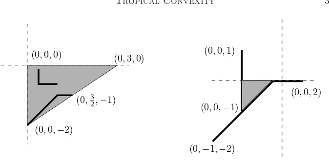
Figure 1: Tropical convex sets and tropical line segments in TP2.
2 Tropically convex sets
We begin with two pictures of tropical convex sets in the tropical planeTP2. A point (x1, x2, x3)∈TP2 is represented by drawing the point with coordinates
(x2−x1, x3−x1) in the plane of the paper. The triangle on the left hand side in
Figure 1 is tropically convex, but it is not a tropical polytope because it is not the tropical convex hull of finitely many points. The thick edges indicate two tropical line segments. The picture on the right hand side is atropical triangle, namely, it is the tropical convex hull of the three points (0,0,1), (0,2,0) and (0,−1,−2) in the tropical plane TP2. The thick edges represent the tropical segments connecting any two of these three points.
We next show that tropical convex sets enjoy many of the features of ordinary convex sets.
Theorem 2. The intersection of two tropically convex sets inRn or inTPn−1
is tropically convex. The projection of a tropically convex set onto a coordinate hyperplane is tropically convex. The ordinary hyperplane {xi −xj = l} is
tropically convex, and the projection map from this hyperplane to Rn−1 given by eliminatingxiis an isomorphism of tropical semimodules. Tropically convex
sets are contractible spaces. The Cartesian product of two tropically convex sets is tropically convex.
Proof. We prove the statements in the order given. If S and T are tropically convex, then for any two pointsx, y∈S∩T, bothSandT contain the tropical line segment betweenxandy, and consequently so doesS∩T. ThereforeS∩T
is tropically convex by definition.
Suppose S is a tropically convex set in Rn. We wish to show that the im-age of S under the coordinate projection φ :Rn →Rn−1,(x
1, x2, . . . , xn) 7→
obvious identity
φ¡
c⊙x⊕d⊙y¢
= c⊙φ(x) ⊕d⊙φ(y).
This means that φ is a homomorphism of tropical semimodules. Therefore, if
S contains the tropical line segment betweenxandy, thenφ(S) contains the tropical line segment between φ(x) and φ(y) and hence is tropically convex. The same holds for the induced map φ:TPn−1→TPn−2.
Most ordinary hyperplanes inRnare not tropically convex, but we are claiming that hyperplanes of the special form xi−xj =k are tropically convex. If x andy lie in that hyperplane then xi−yi=xj−yj. This last equation implies the following identity for any real numbersc, d∈R:
(c⊙x⊕d⊙y)i−(c⊙x⊕d⊙y)j = min (xi+c, yi+d)−min (xj+c, yj+d) =k.
Hence the tropical line segment between x and y also lies in the hyperplane {xi−xj=k}.
Consider the map from {xi −xj = k} to Rn−1 given by deleting the i-th coordinate. This map is injective: if two points differ in the xi coordinate they must also differ in the xj coordinate. It is clearly surjective because we can recover an i-th coordinate by setting xi = xj +k. Hence this map is an isomorphism ofR-vector spaces and it is also an isomorphism of (R,⊕, ⊙)-semimodules.
Let S be a tropically convex set in Rn or TPn−1. Consider the family of hyperplanes Hl = {x1−x2 = l} for l ∈ R. We know that the intersection S∩Hl is tropically convex, and isomorphic to its (convex) image under the map deleting the first coordinate. This image is contractible by induction on the dimensionnof the ambient space. Therefore,S∩Hl is contractible. The result then follows from the topological result that ifS is connected, which all tropically convex sets obviously are, and if S∩Hl is contractible for each l, thenS itself is also contractible.
Suppose that S ⊂ Rn and T ⊂ Rm are tropically convex. Our last assertion states that S×T is a tropically convex subset ofRn+m. Take any (x, y) and (x′
, y′
) in S×T andc, d∈R. Then
c⊙(x, y) ⊕d⊙(x′ , y′
) = ¡
c⊙x⊕d⊙x′
, c⊙y⊕d⊙y′¢
lies inS×T sinceS andT are tropically convex.
We next give a more precise description of what tropical line segments look like.
Proposition3. The tropical line segment between two pointsxandyinTPn−1
Proof. After relabeling the coordinates of x = (x1, , . . . , xn) and y =
(y1, . . . , yn), we may assume
y1−x1 ≤ y2−x2 ≤ · · · ≤ yn−xn. (2) The following points lie in the given order on the tropical segment between x
andy:
x= (y1−x1)⊙x⊕ y = ¡y1, y1−x1+x2, . . . , y1−x1+xn−1, y1−x1+xn¢ (y2−x2)⊙x⊕ y = ¡y1, y2, y2−x2+x3, . . . , y2−x2+xn−1, y2−x2+xn¢ (y3−x3)⊙x⊕ y = ¡y1, y2, y3, . . . , y3−x3+xn−1, y3−x3+xn¢
..
. ... ...
(yn−1−xn−1)⊙x⊕ y = ¡y1, y2, y3, . . . , yn−1, yn−1−xn−1+xn¢
y= (yn−xn)⊙x⊕ y = ¡y1, y2, y3, . . . , yn−1, yn¢.
Between any two consecutive points, the tropical line segment agrees with the ordinary line segment, which has slope (0,0, . . . ,0,1,1, . . . ,1). Hence the tropical line segment between xand y is the concatenation of at mostn−1 ordinary line segments, one for each strict inequality in (2).
This description of tropical segments shows an important feature of tropical polytopes: their edges use a limited set of directions. The following result characterizes the tropical convex hull.
Proposition4. The smallest tropically convex subset ofTPn−1which contains a given setV coincides with the set of all tropical linear combinations (1). We denote this set by tconv(V).
Proof. Let x = Lr
i=1ai⊙vi be the point in (1). Ifr≤2 thenxis clearly in the tropical convex hull ofV. Ifr >2 then we write x = a1⊙v1⊕(Lri=2ai⊙vi). The parenthesized vector lies the tropical convex hull, by induction on r, and hence so doesx. For the converse, consider any two tropical linear combinations
x = Lr
i=1ci⊙vi and y = Lrj=1di⊙vi. By the distributive law, a⊙x⊕b⊙y is
also a tropical linear combination ofv1, . . . , vr∈V. Hence the set of all tropical linear combinations ofV is tropically convex, so it contains the tropical convex hull ofV.
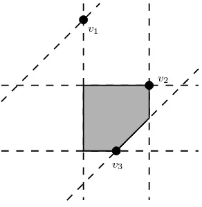
IfV is a finite subset ofTPn−1then tconv(V) is atropical polytope. In Figure 2
we see three small examples of tropical polytopes. The first and second are tropical convex hulls of three points inTP2. The third tropical polytope lies in TP3 and is the union of three squares.
One of the basic results in the usual theory of convex polytopes is Carath´eodory’s theorem. This theorem holds in the tropical setting.
Proposition5(Tropical Carath´eodory’s Theorem). Ifxis in the trop-ical convex hull of a set ofrpointsviinTPn−1, thenxis in the tropical convex
v2= (0,2,0)
v3= (0,1,−2)
v2= (0,2,0)
v1= (0,0,1)
v3= (0,−2,−2)
v1= (0,0,2)
v2= (0,1,0,1)
v3= (0,1,1,0) v1= (0,0,1,1)
Figure 2: Three tropical polytopes. The first two live inTP2, the last inTP3.
Proof. Let x = Lr
i=1ai⊙vi and supposer > n. For each coordinate j ∈ {1, . . . , n}, there exists an index i∈ {1, . . . , r} such that xj =ci+vij. Take a subset I of{1, . . . , r} composed of one suchifor eachj. Then we also have
x = L
i∈Iai⊙vi, where #(I)≤n.
The basic theory of tropical linear subspaces in TPn−1 was developed in [18] and [20]. Recall that thetropical hyperplane defined by a tropical linear form
a1⊙x1 ⊕a2⊙x2 ⊕ · · · ⊕an⊙xn consists of all points x= (x1, x2, . . . , xn) in TPn−1 such that the following holds (in ordinary arithmetic):
ai+xi = aj+xj = min{ak+xk : k= 1, . . . , n} for some indicesi6=j. (3) Just like in ordinary geometry, hyperplanes are convex sets:
Proposition6. Tropical hyperplanes inTPn−1 are tropically convex. Proof. LetH be the hyperplane defined by (3). Suppose thatxandylie inH
and consider any tropical linear combination z = c⊙x ⊕d⊙y. Let ibe an index which minimizes ai+zi. We need to show that this minimum is attained at least twice. By definition, zi is equal to eitherc+xi or d+yi, and, after permuting x and y, we may assume zi = c+xi ≤ d+yi. Since, for allk,
ai+zi ≤ak +zk and zk ≤ c+xk, it follows that ai+xi ≤ ak+xk for all
k, so that ai+xi achieves the minimum of {a1+x1, . . . , an+xn}. Since x is in H, there exists some index j 6=i for which ai+xi =aj+xj. But now
aj+zj≤aj+c+xj =c+ai+xi=ai+zi. Sinceai+zi is the minimum of allaj+zj, the two must be equal, and this minimum is obtained at least twice as desired.
Proposition 6 implies that if V is a subset of TPn−1 which happens to lie in
as well. The same holds for tropical planes of higher codimension. Recall that every tropical plane is an intersection of tropical hyperplanes [20]. But the converse does not hold: not every intersection of tropical hyperplanes qualifies as a tropical plane (see [18, §5]). Proposition 6 and the first statement in Theorem 2 imply:
Corollary 7. Tropical planes inTPn−1 are tropically convex.
A theorem in classical geometry states that every point outside a closed convex set can be separated from the convex set by a hyperplane. The same statement holds in tropical geometry. This follows from the results in [3]. Some caution is needed, however, since the definition of hyperplane in [3] differs from our definition of hyperplane, as explained in [18]. In our definition, a tropical hyperplane is a fan which divides TPn−1 into n convex cones, each of which is also tropically convex. Rather than stating the most general separation theorem, we will now focus our attention on tropical polytopes, in which case the separation theorem is the Farkas Lemma stated in the next section.
3 Tropical polytopes and cell complexes
Throughout this section we fix a finite subset V ={v1, v2, . . . , vr} of tropical projective space TPn−1
. Here vi = (vi1, vi2, . . . , vin). Our goal is to study
the tropical polytope P = tconv(V). We begin by describing the natural cell decomposition of TPn−1induced by the fixed finite subsetV.
Letxbe any point inTPn−1. Thetypeofxrelative toV is the orderedn-tuple (S1, . . . , Sn) of subsets Sj⊆ {1,2, . . . , r} which is defined as follows: An index
iis in Sj if
vij−xj = min(vi1−x1, vi2−x2, . . . , vin−xn).
Equivalently, if we set λi= min{λ∈R : λ⊙vi ⊕x = x} thenSj is the set of all indicesisuch thatλi⊙vi andxhave the same j-th coordinate. We say that ann-tuple of indicesS= (S1, . . . , Sn) is atype if it arises in this manner.
Note that everyimust be in some Sj.
Example 8. Letr =n = 3,v1 = (0,0,2), v2 = (0,2,0) and v3 = (0,1,−2).
There are 30 possible types asxranges over the planeTP2. The corresponding cell decomposition has six convex regions (one bounded, five unbounded), 15 edges (6 bounded, 9 unbounded) and 6 vertices. For instance, the point x= (0,1,−1) has type(x) = ¡
{2},{1},{3}¢
and its cell is a bounded pentagon. The point x′ = (0,0,0) has type(x′) =¡
{1,2},{1},{2,3}¢
and its cell is one of the six vertices. The pointx′′
= (0,0,−3) has type(x′′
) =©
{1,2,3},{1},∅¢
and its cell is an unbounded edge.
Proposition9 (Tropical Farkas Lemma). For allx∈TPn−1, exactly one of the following is true.
(i) the point xis in the tropical polytope P= tconv(V), or (ii) there exists a tropical hyperplane which separatesxfromP.
The separation statement in part (ii) means the following: if the hyperplane is given by (3) and ak +xk = min(a1+x1, . . . , an+xn) then ak +yk > min(a1+y1, . . . , an+yn) for ally∈P.
Proof. Consider any point x ∈ TPn−1, with type(x) = (S
1, . . . , Sn), and let λi= min{λ∈R : λ⊙vi ⊕x = x} as before. We define
πV(x) = λ1⊙v1 ⊕ λ2⊙v2 ⊕ · · · ⊕ λr⊙vr. (4) There are two cases: either πV(x) =x or πV(x)6=x. The first case implies (i). Since (i) and (ii) clearly cannot occur at the same time, it suffices to prove that the second case implies (ii).
Suppose that πV(x) 6= x. Then Sk is empty for some index k ∈ {1, . . . , n}. This means that vik+λi−xk >0 fori= 1,2, . . . , r. Letε >0 be smaller than any of theserpositive reals. We now choose our separating tropical hyperplane (3) as follows:
ak := −xk−ε and aj := −xj for j∈ {1, . . . , n}\{k}. (5) This certainly satisfiesak+xk = min(a1+x1. . . . , an+xn). Now, consider any point y=Lr
i=1ci⊙vi in tconv(V). Pick anymsuch thatyk =cm+vmk. By definition of theλi, we have xk ≤λm+vmk for allk, and there exists somej with xj =λm+vmj. These equations and inequalities imply
ak+yk = ak+cm+vmk = cm+vmk−xk−ε > cm−λm = cm+vmj−xj ≥ yj−xj = aj+yj ≥ min(a1+y1, . . . , an+yn). Therefore, the hyperplane defined by (5) separatesxfrom P as desired. The construction in (4) defines a map πV : TPn−1→P whose restriction to
P is the identity. This map is the tropical version of the nearest point map
onto a closed convex set in ordinary geometry. Such maps were studied in [3] for convex subsets in arbitrary idempotent semimodules.
IfS= (S1, . . . , Sn) andT = (T1, . . . , Tn) aren-tuples of subsets of{1,2, . . . , r},
then we write S⊆T if Sj⊆Tj forj = 1, . . . , n. We also consider the set of all points whose type containsS:
XS := ©x∈TPn
−1 : S ⊆ type(x)ª .
Lemma 10. The set XS is a closed convex polyhedron (in the usual sense).
More precisely,
v1
v2
v3
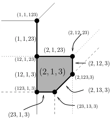
Figure 3: The regionX(2,1,3) in the tropical convex hull ofv1,v2andv3.
Proof. Letx∈TPn−1andT = type(x). First, supposexis inX
S. ThenS⊆T. For everyi, j, k such that i∈Sj, we also havei∈Tj, and so by definition we have vij−xj≤vik−xk, orxk−xj≤vik−vij. Hence xlies in the set on the right hand side of (6). For the proof of the reverse inclusion, suppose that x
lies in the right hand side of (6). Then, for alli, jwithi∈Sj, and for allk, we havevij−xj≤vik−xk. This means that vij−xj= min(vi1−x1, . . . , vin−xn) and hence i∈Tj. Consequently, for allj, we haveSj⊂Tj, and sox∈XS. As an example for Lemma 10, we consider the region X(2,1,3) in the tropical
convex hull of v1 = (0,0,2), v2 = (0,2,0), and v3 = (0,1,−2). This region
is defined by six linear inequalities, one of which is redundant, as depicted in Figure 3. Lemma 10 has the following immediate corollaries.
Corollary 11. The intersection XS∩XT is equal to the polyhedron XS∪T.
Proof. The inequalities definingXS∪T are precisely the union of the inequalities definingXS andXT, and points satisfying these inequalities are precisely those in XS∩XT.
Corollary 12. The polyhedron XS is bounded if and only if Sj 6=∅ for all
j= 1,2, . . . , n.
Proof. Suppose that Sj 6= ∅ for all j = 1,2, . . . , n. Then for every j and k, we can find i ∈ Sj and m ∈ Sk, which via Lemma 10 yield the inequalities
vmk−vmj ≤xk−xj≤vik−vij. This implies that eachxk−xj is bounded on
XS, which means thatXS is a bounded subset of TPn
−1
.
Conversely, suppose someSj is empty. Then the only inequalities involvingxj are of the formxj−xk ≤cjk. Consequently, if any pointxis inSj, so too is
Corollary 13. Suppose we have S = (S1, . . . , Sn), with S1 ∪ · · · ∪Sn = {1, . . . , r}. Then if S ⊆T, XT is a face of XS, and furthermore all faces of
XS are of this form.
Proof. For the first part, it suffices to prove that the statement is true when
T covers S in the poset of containment, i.e. when Tj = Sj ∪ {i} for some
j∈ {1, . . . , n}andi6∈Sj, andTk=Sk fork6=j.
We have the inequality presentation ofXS given by Lemma 10. By the same lemma, the inequality presentation of XT consists of the inequalities defining
XS together with the inequalities
{xk−xj≤vik−vij | k∈ {1, . . . , n}}. (7)
By assumption, iis in someSm. We claim that XT is the face ofSdefined by the equality
xm−xj =vim−vij. (8)
SinceXS satisfies the inequalityxj−xm≤vij−vim, (8) defines a faceF ofS. The inequalityxm−xj≤vim−vij is in the set (7), so (8) is valid onXT and
XT ⊆F. However, any point inF, being inXS, satisfiesxk−xm≤vik−vimfor allk∈ {1, . . . , n}. Adding (8) to these inequalities proves that the inequalities (7) are valid onF, and henceF ⊆XT. SoXT =F as desired.
By the discussion in the proof of the first part, prescribing equality in the facet-defining inequality xk−xj ≤ vik−vij yields XT, where Tk =Sk∪ {i} and
Tj =Sj forj 6=k. Therefore, all facets ofXS can be obtained as regionsXT, and it follows recursively that all faces ofXS are of this form.
Corollary 14. Suppose that S = (S1, . . . , Sn) is an n-tuple of indices
sat-isfying S1∪ · · · ∪Sn = {1, . . . , r}. Then XS is equal to XT for some type
T.
Proof. Let x be a point in the relative interior ofXS, and let T = type(x). Sincex∈XS,T containsS, and by Lemma 13,XT is a face ofXS. However, sincexis in the relative interior ofXS, the only face ofXS containingxisXS itself, so we must haveXS =XT as desired.
We are now prepared to state our main theorem in this section.
Theorem 15. The collection of convex polyhedra XS, where S ranges over
all types, defines a cell decomposition CV of TPn−1. The tropical polytope P = tconv(V) equals the union of all bounded cellsXS in this decomposition.
but XS∩XT =XS∪T by Corollary 11, andXS∪T is a face ofXS and XT by Corollary 13.
For the second assertion consider any point x∈TPn−1 and let S = type(x).
We have seen in the proof of the Tropical Farkas Lemma (Proposition 9) that
xlies inP if and only if noSj is empty. By Corollary 12, this is equivalent to the polyhedronXS being bounded.
The collection of bounded cellsXS is referred to as the tropical complex gen-erated by V; thus, Theorem 15 states that this provides a polyhedral decom-position of the polytope P = tconv(V). Different sets V may have the same tropical polytope as their convex hull, but generate different tropical complexes; the decomposition of a tropical polytope depends on the chosen generating set, although we will see later (Proposition 21) that there is a unique minimal generating set.
Here is a nice geometric construction of the cell decomposition CV of TPn
−1
induced by V ={v1, . . . , vr}. LetFbe the fan inTPn
−1defined by the tropical
hyperplane (3) with a1 =· · · =an = 0. Two vectors xandy lie in the same relatively open cone of the fanF if and only if
{j : xj = min(x1, . . . , xn)} = {j : yj = min(y1, . . . , yn)}.
If we translate the negative ofF by the vectorvi then we get a new fan which we denote by vi− F. Two vectorsxandy lie in the same relatively open cone of the fan vi− F if and only if
{j : xj−vij = max(x1−vi1, . . . , xn−vin)}
= {j : yj−vij = max(y1−vi1, . . . , yn−vin)}.
Proposition16. The cell decomposition CV is the common refinement of the
r fans vi− F.
Proof. We need to show that the cells of this common refinement are precisely the convex polyhedra XS. Take a point x, with T = type(x) and define
Sx= (Sx1, . . . , Sxn) by lettingi∈Sxj whenever
xj−vij = max(x1−vi1, . . . , xn−vin). (9)
Two pointsxandyare in the relative interior of the same cell of the common refinement if and only if they are in the same relatively open cone of each fan; this is tantamount to saying thatSx =Sy. However, we claim thatSx =T. Indeed, taking the negative of both sides of (9) yields exactly the condition for
(2,123,3)
(123,1,3)
(1,1,23)
(12,1,3)
(2,13,3) (2,1,23)
(23,1,3)
(12,1,23)
(2,12,3)
(2
,
1
,
3)
(23,13,3)
(2,12,23)
(1,1,123)
Figure 4: A tropical complex expressed as the bounded cells in the common refinement of the fansv1− F, v2− F andv3− F. Cells are labeled with their
types.
An example of this construction is shown for our usual example, where v1 =
(0,0,2), v2= (0,2,0), andv3= (0,1,−2), in Figure 4.
The next few results provide additional information about the polyhedronXS. Let GS denote the undirected graph with vertices {1, . . . , n}, where{j, k} is an edge if and only if Sj∩Sk6=∅.
Proposition 17. The dimension dof the polyhedron XS is one less than the
number of connected components ofGS, andXS is affinely and tropically
iso-morphic to some polyhedronXT inTPd.
Proof. The proof is by induction onn. Suppose we havei∈Sj∩Sk. ThenXS satisfies the linear equationxk−xj =c where c=vik−vij. Eliminating the variable xk (projecting onto TPn
−2
), XS is affinely and tropically isomorphic toXT where the typeT is defined byTr=Sr forr6=j andTj=Sj∪Sk. The region XT exists in the cell decomposition of TPn
−2
induced by the vectors
w1, . . . , wn with wir =vir forr6=j, and wij = max(vij, vik−c). The graph
GT is obtained from the graphGS by contracting the edge{j, k}, and thus has the same number of connected components.
This induction on n reduces us to the case where all of the Sj are pairwise disjoint. We must show that XS has dimension n−1. Suppose not. Then
XS lies in TPn
−1
Sj andSk are not disjoint, a contradiction.
The following proposition can be regarded as a converse to Lemma 10. Proposition 18. Let R be any polytope in TPn−1 defined by inequalities of the form xk−xj ≤cjk. Then R arises as a cell XS in the decomposition CV
of TPn−1 defined by some setV ={v1, . . . , vn}.
Proof. Define the vectorsvi to have coordinatesvij =cij fori6=j, andvii= 0. (Ifcij did not appear in the given inequality presentation then simply take it to be a very large positive number.) Then by Lemma 10, the polytope inTPn−1
defined by the inequalities xk−xj ≤cjk is precisely the unique cell of type (1,2, . . . , n) in the tropical convex hull of{v1, . . . , vn}.
The region XS is a polytope both in the ordinary sense and in the tropical sense.
Proposition19. Every bounded cellXS in the tropical complex generated by
V is itself a tropical polytope, equal to the tropical convex hull of its vertices. The number of vertices of the polytope XS is at most ¡2nn−−12
¢
, and this bound is tight for all positive integersn.
Proof. By Proposition 17, if XS has dimension d, it is affinely and tropically isomorphic to a region in the convex hull of a set of points inTPd, so it suffices to consider the full-dimensional case.
The inequality presentation of Lemma 10 demonstrates that XS is tropically convex for allS, since if two points satisfy an inequality of that form, so does any tropical linear combination thereof. Therefore, it suffices to show thatXS is contained in the tropical convex hull of its vertices.
The proof is by induction on the dimension of XS. All proper faces of XS are polytopes XT of lower dimension, and by induction are contained in the tropical convex hull of their vertices. These vertices are a subset of the vertices ofXS, and so this face is in the tropical convex hull.
Take any pointx= (x1, . . . , xn) in the interior ofXS. SinceXS has dimension
n, we can travel in any direction fromxwhile remaining inXS. Let us travel in the (1,0, . . . ,0) direction until we hit the boundary, to obtain pointsy1 =
(x1+b, x2, . . . , xn) andy2= (x1−c, x2, . . . , xn) in the boundary ofXS. These points are contained in the tropical convex hull by the inductive hypothesis, which means that x = y1⊕c⊙y2 is also, completing the proof of the first
assertion.
For the second assertion, we consider the convex hull of all differences of unit vectors,ei−ej. This is a lattice polytope of dimensionn−1 and normalized volume ¡2n−2
n−1 ¢
. To see this, we observe that this polytope is tiled byncopies of the convex hull of the origin and the ¡n
2 ¢
[4, Theorem 2.3 (2)] that the normalized volume of this polytope equals the
We conclude that every complete fan whose rays are among the vectorsei−ej has at most ¡2n−2
n−1 ¢
maximal cones. This applies in particular to the normal fan of XS, hence XS has at most ¡2nn−−12
¢
vertices. Since the configuration {ei−ej} is unimodular, the bound is tight whenever the fan is simplicial and uses all the raysei−ej.
We close this section with two more results about arbitrary tropical polytopes in TPn−1.
Proposition 20. If P and Q are tropical polytopes in TPn−1 then P∩Q is also a tropical polytope.
Proof. SinceP andQare both tropically convex,P∩Qmust also be. Conse-quently, if we can find a finite set of points inP∩Qwhose convex hull contains all of P∩Q, we will be done. By Theorem 15, P andQare the finite unions of bounded cells{XS} and{XT} respectively, so P∩Qis the finite union of the cells XS ∩XT. Consider any XS ∩XT. Using Lemma 10 to obtain the inequality representations ofXS andXT, we see that this region is of the form dictated by Proposition 18, and therefore obtainable as a cell XW in some tropical complex. By Proposition 19,XW is itself a tropical polytope, and we can therefore find a finite set whose convex hull is equal to XS∩XT. Taking the union of these sets over all choices ofSandT then gives us the desired set of points whose convex hull contains all ofP∩Q.
Proposition 21. Let P ⊂TPn−1 be a tropical polytope. Then there exists a unique minimal setV such thatP = tconv(V).
If the termf1⊙v1 does not minimize any coordinate in the right-hand side of
(10), thenv1is a linear combination ofv2, . . . , vm, contradicting the minimality
ofV. However, iff1⊙v1minimizes any coordinate in this expression, it must
minimize all of them, since (v1)j−(v1)k = (f1⊙v1)j−(f1⊙v1)k. In this case
we get v1 =f1⊙v1, or f1 = 0. Pick any ifor which f1 =di+ci1; we claim
Like many of the results presented in this section, Propositions 20 and 21 parallel results on ordinary polytopes. We have already mentioned the tropical analogues of the Farkas Lemma and of Carath´eodory’s Theorem (Propositions 5 and 9); Proposition 17 is analogous to the result that a polytope P ⊂ Rn of dimension d is affinely isomorphic to someQ ⊂ Rd. Proposition 19 hints at a duality between an inequality representation and a vertex representation of a tropical polytope; this duality has been studied in greater detail by Michael Joswig [11].
4 Subdividing products of simplices Every set V = {v1, . . . , vr} of r points in TPn
−1 begets a tropical polytope P = tconv(V) equipped with a cell decomposition into the tropical complex generated by V. Each cell of this tropical complex is labelled by its type, which is an n-vector of finite subsets of {1, . . . , r}. Two configurations (and their corresponding tropical complexes)V andW have the samecombinatorial type if the types occurring in their tropical complexes are identical; note that by Lemma 13, this implies that the face posets of these polyhedral complexes are isomorphic.
With the definition in the previous paragraph, the statement of Theorem 1 has now finally been made precise. We will prove this correspondence between tropical complexes and subdivisions of products of simplices by constructing the polyhedral complexCP in a higher-dimensional space.
Let W denote the (r + n − 1)-dimensional real vector space Rr+n/(1, . . . ,1,−1, . . . ,−1). The natural coordinates on W are denoted (y, z) = (y1, . . . , yr, z1, . . . , zn). As before, we fix an ordered subset V = {v1, . . . , vr} of TPn
−1 where v
i = (vi1, . . . , vin). This defines the
unbounded polyhedron PV =
©
(y, z)∈W : yi+zj ≤vij for alli∈ {1, . . . , r}andj ∈ {1, . . . , n}
ª .
(11) Lemma 22. There is a piecewise-linear isomorphism between the tropical com-plex generated by V and the complex of bounded faces of the (r+n−1) -dimensional polyhedron PV. The image of a cell XS of CP under this
iso-morphism is the bounded face {yi+zj = vij : i ∈ Sj} of the polyhedron PV. That bounded face maps isomorphically to XS via projection onto the
z-coordinates.
Proof. LetF be a bounded face ofPV, and defineSj viai∈Sj ifyi+zj =vij is valid on all of F. If some yi or zj appears in no equality, then we can subtract arbitrary positive multiples of that basis vector to obtain elements of
F, contradicting the assumption that F is bounded. Therefore, each i must appear in some Sj, and eachSj must be nonempty.
Since everyyi appears in some equality, given a specific z in the projection of
projection is an affine isomorphism fromF to its image. We need to show that this image is equal toXS.
Letz be a point in the image of this projection, coming from a point (y, z) in the relative interior of F. We claim that z ∈XS. Indeed, looking at thejth coordinate ofz, we find
−yi+vij ≥ zj for alli, (12) −yi+vij = zj for i∈Sj. (13) The defining inequalities ofXS arexj−xk ≤vij−vikwithi∈Sj. Subtracting the inequality−yi+vik≥zkfrom the equality in (13) yields that this inequality is valid on z as well. Therefore, z ∈ XS. Similar reasoning shows that S = type(z). We note that the relations (12) and (13) can be rewritten elegantly in terms of the tropical product of a row vector and a matrix:
z = (−y)⊙V = r
M
i=1
(−yi)⊙vi. (14)
For the reverse inclusion, suppose that z∈XS. We define y=V⊙(−z). This means that
yi = min(vi1−z1, vi2−z2, . . . , vin−zn). (15) We claim that (y, z)∈F. Indeed, we certainly haveyi+zj≤vij for alliandj, so (y, z)∈ PV. Furthermore, wheni∈Sj, we know thatvij−zj achieves the minimum in the right-hand side of (15), so thatvij−zj=yi andyi+zj =vij is satisfied. Consequently, (y, z)∈F as desired.
It follows immediately that the two complexes are isomorphic: if F is a face corresponding toXS andGis a face corresponding toXT, whereS andT are both types, thenXS is a face ofXT if and only ifT ⊆S. However, by the dis-cussion above, this is equivalent to saying that the equalitiesGsatisfies (which correspond to T) are a subset of the equalities F satisfies (which correspond to S); this is true if and only ifF is a face ofG. SoXS is a face ofXT if and only ifF is a face ofG, which implies the isomorphism of complexes.
The boundary complex of the polyhedron PV is polar to the regular subdivision of the product of simplices ∆r−1×∆n−1defined by the weightsvij. We denote this regular polyhedral subdivision by (∂PV)∗. Explicitly, a subset of vertices (ei, ej) of ∆r−1×∆n−1 forms a cell of (∂PV)∗ if and only if the equations
yi+zj =vij indexed by these vertices specify a face of the polyhedronPV. We refer to the book of De Loera, Rambau and Santos [5] for basics on polyhedral subdivisions.
We now present the proof of the result stated in the introduction.
Proof of Theorem 1: The poset of bounded faces ofPV is antiisomorphic to
the poset of interior cells of the subdivision (∂PV)∗ of ∆r−1×∆n−1. Since
every full-dimensional cell of (∂PV)∗ is interior, the subdivision is uniquely
is uniquely determined by the lists of facets containing each bounded face of PV. These lists are precisely the types of regions in CP by Lemma 22. This completes the proof.
Theorem 1, which establishes a bijection between the tropical complexes gener-ated byrpoints inTPn−1
and the regular subdivisions of a product of simplices ∆r−1×∆n−1, has many striking consequences. First of all, we can pick off the
types present in a tropical complex simply by looking at the cells present in the corresponding regular subdivision. In particular, if we have an interior cell
M, the corresponding type appearing in the tropical complex is defined via
Sj ={i∈[n] | (j, i)∈M}.
It is worth noting that via the Cayley Trick [19], Theorem 1 is equivalent to saying that tropical complexes generated byrpoints inTPn−1 are in bijection with the regular mixed subdivisions of the dilated simplexr∆n−1. This
con-nection is expanded upon and employed in a paper with Francisco Santos [6]. Another astonishing consequence of Theorem 1 is the identification of the row span and column span of a matrix. This result can also be derived from [3, Theorem 42].
Theorem 23. Given any matrixM ∈Rr×n, the tropical complex generated by
its column vectors is isomorphic to the tropical complex generated by its row vectors. This isomorphism is gotten by restricting the piecewise linear maps
Rn→Rr, z7→M⊙(−z) and Rr→Rn, y 7→(−y)⊙M.
Proof. By Theorem 1, the matrixM corresponds via the polyhedronPM to a regular subdivision of ∆r−1×∆n−1, and the complex of interior faces of this
regular subdivision is combinatorially isomorphic to both the tropical complex generated by its row vectors, which are r points in TPn−1, and the
tropi-cal complex generated by its column vectors, which are n points in TPr−1. Furthermore, Lemma 22 tells us that the cell in PM is affinely isomorphic to its corresponding cell in both tropical complexes. Finally, in the proof of Lemma 22, we showed that the point (y, z) in a bounded faceF ofPM satisfies
y = M ⊙(−z) and z = (−y)⊙M. This point projects to y and z, and so the piecewise-linear isomorphism mapping these two complexes to each other is defined by the stated maps.
The common tropical complex of these two tropical polytopes is given by the complex of bounded faces of the common polyhedron PM, which lives in a space of dimension r+n−1; the tropical polytopes are unfoldings of this complex into dimensions r−1 and n−1. Theorem 23 also gives a natural bijection between the combinatorial types of tropical convex hulls of r points in TPn−1 and the combinatorial types of tropical convex hulls of n points in TPr−1, incidentally proving that there are the same number of each. This duality statement extends a similar statement in [3].
B
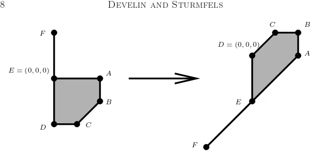
Figure 5: A demonstration of tropical polytope duality.
a tropical triangle (here r=n= 3). For instance, we compute:
This point is the image of the point (0,0,2) under this duality map. Note that duality does not preserve the generating set; the polytope on the right is the convex hull of points {F, D, B}, while the polytope on the left is the convex hull of points{F, A, C}. This is necessary, of course, since in general a polytope withr vertices is mapped to a polytope withnvertices, and rneed not equal
nas it does in our example.
We now discuss the generic case when the subdivision (∂PV)∗ is a regular tri-angulation of ∆r−1×∆n−1. We refer to [18,§5] for the geometric interpretation
of thetropical determinant.
Proposition 24. For a configuration V of r points in TPn−1 with r≥n the following are equivalent:
1. The regular subdivision(∂PV)∗
is a triangulation of ∆r−1×∆n−1. 2. Nokof the points inV have projections onto ak-dimensional coordinate
subspace which lie in a tropical hyperplane, for any2≤k≤n.
3. No k×k-submatrix of the r×n-matrix (vij) is tropically singular, i.e.
has vanishing tropical determinant, for any2≤k≤n.
The regular subdivision (∂PV)∗is a triangulation if and only if the polyhedron
PV is simple, which is to say if and only if nor+nof the facetsyi+zj ≤vij meet at a single vertex. For each vertex v, consider the bipartite graph Gv consisting of verticesy1, . . . , yn and z1, . . . , zj with an edge connecting yi and
zj ifv lies on the corresponding facet. This graph is connected, since each yi andzj appears in some such inequality, and thus it will have a cycle if and only if it has at leastr+nedges. Consequently,PV is not simple if and only there exists someGv with a cycle.
If there is a cycle, without loss of generality it reads y1, z1, y2, z2, . . . , yk, zk. Consider the submatrixM of (vij) given by 1≤i≤kand 1≤j≤k. We have
y1+z1=M11,y2+z2=M22, and so on, and alsoz1+y2=M12, . . . , zk+y1= Mk1. Adding up all of these equalities yields y1+· · ·+yk+z1+· · ·+zk =
M11+· · ·+Mkk = M12+· · ·+Mk1. But consider any permutation σ in
the symmetric group Sk. Since we haveMiσ(i) =viσ(i)≥yi+zσ(i), we have P
Miσ(i)≥x1+· · ·+xk+y1+· · ·+yk. Consequently, the permutations equal
to the identity and to (12· · ·k) simultaneously minimize the determinant of the minorM. This logic is reversible, proving the equivalence of (1) and (3).
If therpoints ofV are in general position, the tropical complex they generate is called ageneric tropical complex. These polyhedral complexes are then polar to the complexes of interior faces of regular triangulations of ∆r−1×∆n−1.
Corollary25. All tropical complexes generated byrpoints in general position inTPn−1have the samef-vector. Specifically, the number of faces of dimension k is equal to the multinomial coefficient
µ
r+n−k−2
r−k−1, n−k−1, k ¶
= (r+n−k−2)! (r−k−1)!·(n−k−1)!·k!.
Proof. By Proposition 24, these objects are in bijection with regular triangula-tions ofP = ∆r−1×∆n−1. The polytopeP is equidecomposable [1], meaning
that all of its triangulations have the same f-vector. The number of faces of dimensionkof the tropical complex generated by givenrpoints is equal to the number of interior faces of codimension kin the corresponding triangulation. Since all triangulations of all products of simplices have the samef-vector, they must also have the same interior f-vector, which can be computed by taking thef-vector and subtracting off thef-vectors of the induced triangulations on the proper faces of P. These proper faces are all products of simplices and hence equidecomposable, so all of these induced triangulations have f-vectors independent of the original triangulation as well.
is an intervalIi, and that ifi < m, the intervalsImandIimeet in at most one point, which in that case is the largest element ofImand the smallest element ofIi.
Suppose we have i∈Sj andm∈Sl with i < m. Then we have by definition
vij −xj ≤vil−xl andvml−xl ≤vmj−xj. Adding these inequalities yields
vij +vml ≤vil+vmj, or ij+ml≤il+mj. Since i < m, it follows that we must havel≤j. Therefore, we can never havei∈Sj andm∈Slwith i < m andj < l. The claim follows immediately, since theIi cover [1, n].
The number of degrees of freedom of an interval set (I1, . . . , Ir) is easily seen
to be the number of ifor whichIi andIi+1 are disjoint. Given this, it follows
from a simple combinatorial counting argument that the number of interval sets with k degrees of freedom is the multinomial coefficient given above. Finally, a representative for every interval set is given by xj =xj+1−cj, where if Sj and Sj+1 have an element i in common (they can have at most one),cj =i, and if not thencj = (min(Sj) + max(Sj+1))/2. Therefore, each interval set is
in fact a valid type, and our enumeration is complete.
Corollary 26. The number of combinatorially distinct generic tropical com-plexes generated by r points in TPn−1 equals the number of distinct regular triangulations of ∆r−1×∆n−1. The number of respective symmetry classes under the natural action of the product of symmetric groups G=Sr×Sn on
both spaces is also the same.
The symmetries in the groupGcorrespond to a natural action on ∆r−1×∆n−1
given by permuting the vertices of the two component simplices; the symmetries in the symmetric group Sr correspond to permuting the points in a tropical polytope, while those in the symmetric groupSn correspond to permuting the coordinates. (These are dual, as per Corollary 23.) The number of symmetry classes of regular triangulations of the polytope ∆r−1×∆n−1 is computable
via J¨org Rambau’s TOPCOM [17] for small randn:
2 3
2 5 35
3 35 7,955
4 530
5 13,631
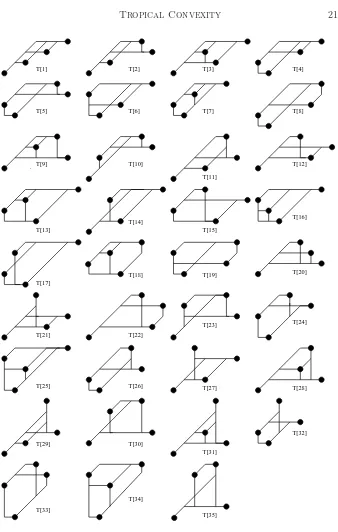
For example, the (2,3) entry of the table divulges that there are 35 symme-try classes of regular triangulations of ∆2×∆3. These correspond to the 35
T[28] T[27]
T[2] T[1]
T[26]
T[23]
T[22]
T[25]
T[24]
T[32]
T[31]
T[35] T[34]
T[33]
T[4] T[3]
T[30] T[29]
T[10] T[9]
T[13]
T[11]
T[12] T[6]
T[5] T[7] T[8]
T[18] T[20]
T[21]
T[19] T[15] T[14]
T[17]
T[16]
5 Phylogenetic analysis using tropical polytopes
A fundamental problem in bioinformatics is the reconstruction of phylogenetic trees from approximate distance data. In this section we show how tropical convexity might help provide new algorithmic tools for this problem. Our ap-proach augments the results in [20,§4] and it provides a tropical interpretation of the work onT-theory by Andreas Dress and his collaborators [7], [8], [9]. Consider a symmetric n×n-matrix D = (dij) whose entries dij are non-negative real numbers and whose diagonal entries dii are all zero. We say that
D is a (finite) metric if the triangle inequality dij ≤ dik+djk holds for all indicesi, j, k. Our starting point is the following easy observation:
Proposition27. The symmetric matrixD is a metric if and only if all prin-cipal3×3-minors of the negated symmetric matrix −D= (−dij) are tropically singular.
Proof. Both properties involve only three points, so we may assumen= 3, in which case
−D =
0 −d12 −d13
−d12 0 −d23
−d13 −d23 0
.
The tropical determinant of this matrix is the minimum of the six expressions 0,−2d12,−2d13,−2d23,−d12−d13−d23 and −d12−d13−d23.
This minimum is attained twice if and only if it is attained by the last two (identical) expressions, which occurs if and only if the three triangle inequalities are satisfied.
In what follows we assume that D = (dij) is a metric. Let PD denote the tropical convex hull in TPn−1 of the n row vectors (or column vectors) of the negated matrix −D = (−dij). Proposition 27 tells us that the tropical polytopePDis always one-dimensional for n= 3.
The finite metricD= (dij) is said to be atree metricif there exists a weighted tree T with n leaves such that dij denotes the distance between the i-th leaf and the j-th leaf along the unique path between these leaves in T. The next theorem characterizes tree metrics among all metrics by the dimension of the tropical polytopePD. It is the tropical interpretation of results that are quite classical and well-known in the phylogenetics literature.
Theorem 28. For a given finite metricD= (dij)the following conditions are
equivalent:
1. D is a tree metric,
2. the tropical polytopePD has dimension one,
4. all principal4×4-minors of the matrix −D are tropically singular, 5. For any choice of four indices i, j, k, l ∈ {1,2, . . . , n}, the maximum of
the three numbers dij+dkl, dik+djl and dil+dik is attained at least
twice.
Proof. The condition (5) is the familiarFour Point Conditionfor tree metrics. The equivalence of (1) and (5) is a classical result due to various authors, including Buneman [2] and Zaretsky [21]. See equation (B3) on page 57 in [7]. Suppose that the condition (5) holds. By the discussion in [20,§4], this means that −D is a point in the tropical Grassmannian of lines, in symbols −D ∈ Gr(2, n) ⊂ TP(
n
2). By [20, Theorem 3.8], the point −D corresponds to a
tropical line LD in TPn−1. Thendistinguished points whose coordinates are the rows of−Dlie on the lineLD. By Corollary 7, it follows that their tropical convex hull PD is contained inLD. This means that PD has dimension one, that is, (2) holds.
Suppose that (2) holds. Then the tropical rank of the matrix −D is equal to two, by [6, Theorem 4.2]. This means that allr×r-minors of−Dare tropically singular forr≥3. The caser= 4 is precisely the statement (3).
Obviously, the condition (3) implies the condition (4). What remains is to prove the implication from (4) to (5). For this we note that the tropical determinant of the 4×4-matrix
tropicalization of a 4×4-Pfaffian). The matrix is tropically singular if and only if the minimum is attained twice.
If the five equivalent conditions of Theorem 28 are satisfied then the metric tree
T coincides with the one-dimensional tropical polytope PD. To make sense of this statement, we regard tropical projective space TPn−1 as a metric space with respect to the infinity norm induced fromRn,
||x−y|| = max©
|xi+yj−xj−yi| : 1≤i < j≤nª,
and we note that the finite metricDembeds isometrically intoPDvia the rows of−1
2D:
i 7→ 1
2 ·(−di1,−di2,−di3, . . . ,−din) fori= 1,2, . . . , n
Theorem 29. The tropical polytope PD equals Isbell’s injective hull of the
metricD.
Proof. According to Lemma 22, the tropical polytopePDis the bounded com-plex of the following unbounded polyhedron in the (2n−1)-dimensional space
W =R2n/R(1, . . . ,1,−1, . . . ,−1):
P−D = ©(y, z)∈W : yi+zj ≤ −dij for all 1≤i, j≤nª. Dress et al. [7] showed that the injective hull T(D) of the finite metric D
coincides with the complex of bounded faces of the following n-dimensional unbounded polyhedron:
Q−D = ©x∈Rn : xi+xj≥dij for all 1≤i, j≤nª.
What we need to show is that the two polyhedra have the same bounded complex.
The metricD satisfies the tropical matrix identity −D = D⊙(−D), because −dij = mink(dik−dkj). This implies that any column vectoryof−Dsatisfies
y = (−y)⊙(−D).
Consider any vertex (y, z) ofP−D. Thenyis a column vector of−D. Equation
(14) implies z = (−y)⊙(−D) = y. Hence every vertex of P−D lies in the subspace defined byy=z, and so does the complex of bounded faces ofP−D.
Therefore the linear map (y, z) 7→ −y induces an isomorphism between the bounded complex of P−D and the bounded complex of Q−D.
Theorem 23 specifies an involution on the set of all tropical complexes. We are interested in the fixed points of this canonical involution. A necessary condition is thatr=nand V is a symmetric matrix. The previous result and its proof can be reinterpreted as follows:
Corollary 30. A tropical complex P is pointwise fixed under the canonical involution (on the set of all tropical complexes) if and only ifP is the injective hull of a metric on {1,2, . . . , n}.
The dimension of the tropical complex PD= tconv(−D) can be characterized combinatorially by tropicalizing the sub-Pfaffians of a skew-symmetric n×n -matrix. The tropical Pfaffians of format 4×4 specify the four point condition (5) in Theorem 28, while the tropical sub-Pfaffians of format 6×6 specify the six-point condition which is discussed in [7, page 25]. The combinatorial study ofk-compatible split systems can be interpreted in the setting of tropical algebraic geometry (cf. [15], [18], [20]) as the study of the k-th secant variety
in the Grassmannian Gr(2, n)⊂TP(
n
2).
Tropical convexity provides a convenient language to study numerous exten-sions of the classical problem of tree reconstruction. As an example, imagine the following scenario, which would correspond to the Grassmannian of planes in TPn−1, denoted Gr(3, n).
Suppose there arentaxa, labeled 1,2, . . . , n, and rather than having a distance for any pair i, j, we are now given a proximity measure dijk for any triple
i, j, k∈ {1,2, . . . , n}. We can then construct a tropical polytope by taking the tropical convex hull of ¡n
2 ¢
points as follows:
P = tconv© ¡
−dij1,−dij2,−dij3, . . .−dijn
¢
∈TPn−1 : 1≤i < j≤nª .
Under certain hypotheses, the tropical polytopeP can be realized as the com-plex of bounded faces of the polyhedron in Rn defined by the inequalities
xi+xj+xk ≥ dijk. It provides a polyhedral model for the tree-like nature of the data (dijk). The case of most interest is whenP is two-dimensional in which case it plays the role of atwo-dimensional phylogenetic tree.
The construction of this particular tropical polytopeP was pioneered by Dress and Terhalle in the important paper [9]. There they discussvaluated matroids, which are essentially the points on the tropical Grassmannian of [20], and they call P the tight span of a valuated matroid. We share their view that these tropical polytopes constitute a promising tool for phylogenetic analysis.
Acknowledgements
This work was conducted while Mike Develin held the AIM Postdoctoral Fel-lowship 2003-2008 and Bernd Sturmfels held the MSRI-Hewlett Packard Pro-fessorship 2003/2004. Sturmfels also acknowledges partial support from the National Science Foundation (DMS-0200729).
References
[2] P. Buneman: A note on metric properties of trees,Journal of Combinato-rial Theory, Ser. B 17(1974) 48–50.
[3] G. Cohen, S. Gaubert, and J.-P. Quadrat: Duality and separation theo-rems in idempotent semimodules,arXiv:math.FA/0212294.
[4] I.M. Gel’fand, M.I. Graev and A. Postnikov: Combinatorics of hypergeo-metric functions associated with positive roots, inArnold-Gel’fand Math-ematical Seminars, Geometry and Singularity Theory, (Eds. V.I. Arnold, I.M. Gel’fand, M. Smirnov and V.S. Retakh), Birkh¨auser, Boston, 1997, pp. 205–221.
[5] J. De Loera, J. Rambau and F. Santos: Triangulations of Point Config-urations, Algorithms and Computation in Mathematics, Springer Verlag, Heidelberg, to appear.
[6] M. Develin, F. Santos and B. Sturmfels: On the rank of a tropical matrix,
arXiv:math.CO/0312114.
[7] A. Dress, K.T. Huber and V. Moulton: An explicit computation of the injective hull of certain finite metric spaces in terms of their associated Buneman complex,Advances in Mathematics168(2002) 1–28.
[8] A. Dress, V. Moulton and W. Terhalle: T-Theory – an overview,European Journal of Combinatorics 17(1996) 161–175.
[9] A. Dress and W. Terhalle: The tree of life and other affine buildings. Pro-ceedings of the International Congress of Mathematicians, Vol. III (Berlin, 1998),Documenta Mathematica, Extra Vol. III, 1998, 565–574.
[10] J. Isbell: Six theorems about metric spaces, Comment. Math. Helv. 39 (1964) 65–74.
[11] M. Joswig: Tropical halfspaces,arXiv:math.CO/0312068.
[12] A.N. Kirillov: Introduction to tropical combinatorics, inPhysics and Com-binatorics 2000, Proceedings of the Nagoya 2000 International Workshop, (Eds. A.N. Kirillov and N. Liskova), pp. 82–150, World Scientific, 2001. [13] G. Litvinov, V. Maslov, and G. Shpiz: Idempotent functional
anal-ysis: an algebraic approach, Mathematical Notes 69 (2001) 696–729,
arXiv:math.FA/0009128.
[14] J. Matouˇsek, On directional convexity, Discrete and Computational Ge-ometry 25(2001) 389–403.
[16] M. Noumi and Y. Yamada: Tropical Robinson-Schensted-Knuth corre-spondence and birational Weyl group actions,arXiv:math-ph/0203030. [17] J. Rambau: TOPCOM (Triangulations of Point Configurations and
Ori-ented Matroids), software available at
http://www.zib.de/rambau/TOPCOM/. The numbers cited for
reg-ular triangulations of products of simplices can be found at
http://www.zib.de/rambau/TOPCOM/TOPCOM-examples/.
[18] J. Richter-Gebert, B. Sturmfels, and T. Theobald: First steps in tropical geometry,arXiv:math.AG/0306366, to appear inIdempotent Mathematics and Mathematical Physics, Proceedings Vienna 2003, (editors G.L. Litvi-nov and V.P. Maslov), American Mathematical Society, 2004.
[19] F. Santos: The Cayley Trick and triangulations of products of simplices,
arXiv:math.CO/0312069.
[20] D. Speyer and B. Sturmfels: The tropical Grassmannian,
arXiv:math.AG/0304218, to appear inAdvances in Geometry.
[21] K.A. Zaretsky: Reconstruction of a tree from the distances between its pendant vertices,Uspekhi Math. Nauk. Russian Mathematical Surveys 20 (1965) 90–92.
Mike Develin
American Inst. of Math 360 Portage Ave.
Palo Alto, CA 94306-2244 USA
Bernd Sturmfels Dept. of Mathematics UC-Berkeley
Berkeley, CA 94720 USA