John Salerian, Tendai Gregan, and Ann Stevens, Productivity Commission, Australia
The technical characteristics of electricity generation and transmission have implications for the way in which economic principles are adapted to evaluate pricing and regulation issues in electricity markets. In particular, there is an externality associated with the way in which electricity flows in networks because of Kirchoff’s laws. In this paper, a mathematical programming model is presented that simulates acompetitive electricity market, based on the spatial-intertemporal equilibrium models pioneered by Takayama and Judge (1971). The model is used to simulate the operation of a hypothetical electricity market, illustrating some of the issues arising from the network externality. 2001 Society for Policy Model-ing. Published by Elsevier Science Inc.
1. INTRODUCTION
Australia is in the process of establishing a national electricity market. The objective is to develop a market that operates as close as possible to the concept of economic efficiency by creating competition in those components that are contestable. However, the technical nature of electricity production and transmission still requires a significant amount of regulation to create and run an electricity market that produces market outcomes consistent with economic efficiency.
The way in which the market is regulated can affect the degree to which the operation of the market is economically efficient. In addition to short-term efficiency considerations, the operation of the market has important consequences for the way in which the
Address correspondence to Dr. John Salerian, Productivity Commission, LB2 Collins Street East, Melbourne, Victoria 8003, Australia; E-mail address: [email protected].
The views expressed in this paper are those of the authors and should not be attributed to the Productivity Commission. The authors would like to acknowledge the assistance provided by Ian Hartley and Colin Parker of TransGrid and Bob Waddell and Charles Popple of the Victorian Power Exchange.
Received September 1997; final draft accepted March 1998.
Journal of Policy Modeling22(7):859–893 (2000)
augmentation of both transmission and generation takes place. One important issue is whether the design of the electricity market leads to an efficient system of transmission and generation in the long run.
Recently, there has been an increase in research relating to regulation of the industry and pricing issues, particularly on the pricing of electricity transmission in networks (Bushnell and Stoft, 1996; Chao and Peck, 1996; Wu et al., 1996). A theme emerging from these articles is that some of the principles underlying
propos-als on the regulation of electricity markets are so-calledfolk
theo-rems.That is, they are commonly accepted assertions about the economic principles that, in fact, do not apply to the electricity market. Wu et al. (1996) claimed that these assertions arise because the economic principles being applied to the electricity market are borrowed from other applications of economics, such as transport economics. However, the technology of electricity production and transmission is such that the use of principles from other applica-tions is inappropriate.
This paper aims to illustrate the economic principles embodied in an economically efficient electricity market through the use of a mathematical programming model.
In the model presented here, the power flow equations and variables for a network are included, based on the methodology outlined in Chao and Peck (1996). This paper extends their work by introducing time-specific demand and supply for electricity and allowing the transmission network structure to be varied. A theoretical model is used to analyze how an economically efficient market would price electricity in these circumstances.
A numerical version of this model is then solved to illustrate some of the economic principles.
The structure of the paper is as follows. The mathematical programming methodology is outlined in Section 2. Section 3 formally describes the model used here, and derives the pricing rules necessary for long-run economic efficiency. To set the scene for the numerical example, Section 4 presents the structure of a hypothetical electrical market. Sections 5, 6, and 7 outline the methods relating to demand, transmission, and production of elec-tricity. The results are discussed in Section 8, and Section 9 is the conclusion and suggestions for further research.
2. MATHEMATICAL PROGRAMMING METHODOLOGY
of perfectly competitive equilibria among spatially separated mar-kets. This provided the opportunity to use mathematical program-ming to simulate market behaviour. Later, Takayama and Judge (1971) significantly extended the applicability of the technique by showing that the competitive and monopoly models could be formulated as quadratic programming models.
They also showed that two alternative formulations—the quan-tity formulation (primal), and the price formulation (the purified dual of the primal)—could be used to compute market
equilib-rium.1 Takayama and Woodland (1970) proved the equivalence
between these two formulations. Takayama and Judge (1971) also showed that the quantity and price formulations could be combined to form another maximization problem where both quantity and price are explicit variables in the model. This is thegeneral formulation referred to by MacAulay (1992), and is
sometimes referred to as theself-dualorprimal-dualformulation.
Takayama and Judge (1971) also refer to it as thenet social revenue
formulation. The model presented here has been solved for three formulations—quantity (primal), the dual to the nonlinear primal as described in Balinski and Baumol (1968), and the primal-dual. The general formulation (primal-dual) has wider applicability than either the quantity formulation (primal) or price formulation (dual). For example, it applies where interdependent demand functions do not satisfy the intergrability condition (that is there is no unique solution to their integration), or where policy imposes constraints on both prices and quantities.
In this particular study, the quantity formulation has advantages over the general formulation. First, it reduces the number of vari-ables and equations, which is important when dealing with large-scale models. Second, it is easier to explain the technique and develop and implement the model. This is important, when the time to complete the study is short. For similar reasons, the quan-tity formulation has advantages over other related techniques used to compute economic equilibria, such as nonlinear complementary programming and computable general equilibrium models.
In electricity markets, cost and demand conditions vary by time and from place to place. For example, electricity demand can be met by generation from a range of technologies (gas and coal) and
a range of plant sizes, all connected by a network of transmission. Therefore, spatial-temporal models, which include elements of networks, are particularly useful to capture this complexity.
Theoretical developments and the application of this methodol-ogy to study pricing and deregulation in spatial energy markets increased during the 1980s. Some examples include Salerian (1992), Kolstad (1989), Provenzano (1989), Uri (1983, 1989), Hobbs and Schuler (1985), and Sohl (1985).
In the mathematical programming model developed here, the supply of electricity is represented by economic-engineering mod-els of power stations and transmission lines. Mathematical pro-gramming has been widely applied in modeling electricity supply, primarily to evaluate the least-cost options to meet forecast de-mand. That is, demand is exogenously specified for these models. Examples include Munasinghe (1990), Scherer (1977), and Turvey and Anderson (1977). Two Australian applications of note are ABARE’s version of the MENSA model (Dalziell, Noble, and Ofei-Mensah, 1993) and CSIRO’s earlier version of the MENSA model (Stocks and Musgrove, 1984).
An advantage of the model presented here is that the quantity demanded (and implicitly price) is endogenous to the model.
3. MATHEMATICAL MODEL
This section formally describes the model used in this study. As mentioned in the previous section, the model presented here simulates the long-run market equilibrium. The model represents a hypothetical electricity market that could involve 12 generators distributed around a possible network consisting of four nodes and five links. Demand for electricity takes place at two of the nodes, and generation can take place at three of the nodes. The model represents an annual market consisting of 34 time periods— that is, the 8760 hours in the year have been allocated to 34 time periods (load blocks).
The model has nonlinear variables in both the objective function and constraints. It also includes variables that may have negative or positive values (that is, they are unconstrained in sign).
3A. Notation
GAMS2source code used to generate the model, which is available
from the authors on request.
Sets
b 1, . . . , 34 Time blocks in which electricity is demanded.
n 1, . . . , 4 Nodes on network.
np 1, . . . , 4 Nodes on network.
p 1, . . . , 12 Power stations.
s 1, . . . , 5 Transmission corridors.
Primal variables
NSW Net social welfare.
QDb,n Demand for power at node nin each block b(PWh).
QGCp Installed capacity of each plant p (GW).
QGOb,p Output of plant pin load block b (GW).
QTCs Number of lines of a given capacity in each transmission
corridor s.
QSb,n Electricity generated at node n in load block b from
generators located at the node (GW).
QPb,n,np Quantity of power flow in load blockbon an individual
line, leaving (arriving at) node n for (from) node np
(GW).
db,n,np Difference between phase angles over a transmission
corridor linking nodesn and np in load blockb.
ub,n Voltage phase angle at node n in load bock b, for all
nodes except node 1.
Lagrangian variables
Sb,n,np Shadow price of the equation defining the difference in
phase angles between nodes n and np (Equation 5).
Ts Shadow price of constraint on the maximum number of
power lines that can be erected between two nodes along
transmission corridor s (Equation 9).
Ub,n Shadow price of balancing demand and supply at node
n in block b(Equation 4).
Vb,p Shadow price of balancing the generation of power
sta-tionpin blockb with its installed capacity (Equation 2).
Wp Shadow price of the limit on installed capacity of power
station p (Equation 3).
Xb,n,np Shadow price of power flows between nodes n and np
(in block b) obeying Kirchoff’s laws (Equation 6).
Yb,n Shadow price of electricity at node nin block b
(Equa-tion 7).
Zb,n,np Shadow price in block b of the capacity limit of each
power line connecting nodento node np(Equation 8).
Parameters
kn,np Maximum capacity of each line connecting nodes nand
np (GW).
js Maximum number of lines along transmission corridors.
ab,n Constants for inverse demand curve in blockbat noden.
cb,n Slope of inverse demand for electricity at nodenin blockb.
mb,p Variable costs ($m/MW) of station pin block b.
dp Fixed cost ($m/MW) of plantp.
ts Annualized fixed cost of constructing one transmission
line on links.
u 1000. Scalar for converting GW to MW.
ep Generation unit availability factor (15100% availability
of all units at station).
fp Maximum generation capacity of station p.
aan,np Parameters on the power flow equations.
bbn,np ccn,np
rb 1000 divided by hours of duration in block b, converts
PWh to GW.
3B. The Primal Model
Objective function ($ million):
NSW5o
bon
(ab,nQDb,n11 2cb,nQD
2 b,n)2o
bop
mb,pQGOb,p2o p
dpQGCp2o s
tsQTCs (1)
so that the location and capacity of both generation and transmis-sion are to be optimized.
Energy generation installed capacity balance (GW):
QGOb,p<epQGCp forb,p (2)
This equation limits the output of each power station in any time period to the amount of capacity installed.
Maximum plant generation capacity (GW):
QGCp<fp forp (3)
The amount of capacity installed for each plant is limited by fp
the maximum number of units allowed times the rated generation capacity of each unit.
Nodal electrical generation (MW):
QSb,n2
o
pQGOb,p<0 forb,n (4)
The amount of electricity generated at each node in each load block is limited by the output of all power stations generating electricity at that node in the load block.
Phase-angle difference (radians):
db,n,np2 ub,n1 ub,np50 forb,n,np (5)
This is the difference in the phase angles between two nodes,
nand np, which form a link. The phase angles and the difference
in phase angles are free variables, being unconstrained in sign.
There are onlyn21 independent phase angles, and so the phase
angle at node one is set to zero.
Equation 5 and the following real power-flow equation encapsu-late Kirchoff’s laws on the flow of electricity in networks (see Section 6 for further explanation).
Real power flow (MW):
uQPb,n,np2bbn,npdb,n,np2ccn,npd2b,n,np5aan,np forb,n,np (6)
variables at each end of the line is the total transmission loss along the line.
Supply and demand (GW):
rbQDb,n2QSb,n1
o
npQPb,n,npQTCs<0 forb,n (7)
The quantity of electricity demanded at the node in any time period is limited to the quantity of electricity generated at the node and the net sum of electricity imported and exported by lines connected to the node.
Transmission line capacity (GW):
uQPb,n,np<kn,np forb,n,np (8)
In any load block, the total amount of power flowing along an individual line connecting two nodes is limited to the maximum (thermal) capacity of that line.
Maximum number of lines:
QTCs<js fors (9)
The number of transmission lines along a corridor connecting two nodes is limited to the maximum number of lines the corridor can accommodate.
Non-negative and free variables:
QTC,QD,QGO,QGC,QS>0; QP,u,dare free variables.
3C. Economic Interpretation of the Kuhn-Tucker Conditions
The Kuhn-Tucker conditions for the existence of a solution show the economic principles embodied in the model. They con-tain information on the pricing of electricity at all nodes of the network, the economic dispatch of power stations, the effects of transmission losses on the operation of the system, and the manner in which the capital costs of generation and transmission are recov-ered. The Kuhn-Tucker conditions are derived from the following Langrangian model. To avoid repetition, the Kuhn-Tucker condi-tions in the form of the original primal constraints (Equacondi-tions 2 to 9) are not repeated here.
Lagrangian of the primal problem:
Max L5
o
b
o
nab,nQDb,n121cb,nQD2b,n
2
o
b
o
pmb,pQGOb,p2
o
pdpQGCp2
o
s1
o
b
o
pVb,p
se
pQGCp2QGOb,pd
1
o
p
Wp
sf
p2QGCpd
1o
bo
nUb,n
1
o
pQGOb,p2QSb,n
2
1
o
b
o
no
npSb,n,np
s
ub,n2 ub,np2 db,n,npd
1
o
b
o
no
npXb,n,np
saa
n,np1bbn,npdb,n,np1ccn,npd2b,n,np2uQPb,n,npd
1
o
b
o
nYb,n
1
QSb,n2o
np(QPb,n,npQTCs)2rbQDb,n
2
1
o
b
o
no
npZn,np(kn,np2uQPb,n,np)1
o
sTs(js2QTCs)
QTC,QD,QGO,QGC,QS,T,U,V,W,Y,Z>0; QP,u,d,X,Sfree (10)
]L ]QDb,n
5ab,n1cb,nQDb,n2rbYb,n<0 forb,nand
1
]L]QDb,n
2
QDb,n5(ab,n1cb,nQDb,n2rbYb,n)QDb,n50 forb,n (11)
Equation 11 states that when the quantity of electricity
de-manded is positive for a load block, the nodal price (Yb,nrb) is
equal to the price that consumers are willing to pay for a unit of energy at that node as given by the linear demand function.
]L ]QSb,n
5 2Ub,n1Yb,n<0 forb,nand
1
]L]QSb,n
2
QSb,n5(2Ub,n1Yb,n)QSb,n50 forb,n (12)
Equation 12 states that when power is generated at a node in
a load block, the nodal price (Yb,n) is equal to the (shadow) price
of supply (Ub,n) at that node.3If there is no local generation at a
node, then the nodal price can be less than the supply price. This equation also means that if generation takes place at the node, then the total revenue received for electricity generated at the
node (Yb,nQSb,n) equals the revenue paid to the generators at the
node (Ub,nQSb,n).
]L ]QGOb,p
5 2mb,p2Vb,p1Ub,n<0 forb,pand
1
]L]QGOb,p
2
QGOb,p5(2mb,p2Vb,p1Ub,n)QGOb,p50 forb,p (13)
Equation 13 states that when a plant p (located at node n) is
generating electricity, the supply price (Ub,n) at the node is equal
to the operating cost of the power station (mb,n) plus the rent (Vb,p)
earned because its installed capacity is fully utilized in this period. The rent occurs when the power station is operating but it is not the marginal plant being dispatched on the network. This means the price received exceeds the operating cost of production (short run
marginal cost). The rents,V, represent a contribution to capacity
cost. When the plant is the system marginal plant dispatched, the nodal price equals the plant’s short-run marginal cost of produc-tion. This condition also shows that the revenue paid to an individ-ual power station is eqindivid-ual to the total operating cost plus the rent accrued, because its generating capacity is limiting in that time period.
]L
]QGCp
5 2dp1
o
b
epVb,p2Wp<0 forpand
1
]L]QGCp
2
QGCp5
1
2dp1o
b
epVb,p2Wp
2
QGCp50 forp (14)Equation 14 states that the sum of the profits or rents [that is, the extent to which the nodal (supply) price exceeds the plant marginal cost] for all load blocks, should equal the unit capital cost of the power station plus any rent it accrues because its installed capacity is limited by the maximum allowed. Plant capac-ity is installed only if the cost of the capaccapac-ity can be recovered. However, if there is a restriction on installed capacity that is binding, then the imputed value or opportunity cost of capacity can exceed its unit construction cost. Equations 14 and 13 form the typical peak-load pricing approach used to determine the optimal mix of power stations on the system.
]L
]ub,n5
o
np(Sb,n,np2Sb,n,np)50 forb,n?1 (15)
phase angle is defined in the next equation. Equation 15 illustrates the network externality. It can be thought of as a zero profit condition, so that there are no gains to be made by adjusting phase angles and changing power flows (arbitrage), taking into account that adjusting one power flow causes simultaneous
adjust-ments in other power flows.4
]L
]db,np5 2Sb,n,np1(bbn,np22ccn,npdb,n,np)Xb,n,np50 forb,n,np (16)
Equation 16 states that the (shadow) price of a difference in phase angle over a line is equal to the marginal power flow (with respect to the difference in the phase angle) times the (shadow) price of power flow along a single line.
]L
]QPb,n,np
5 2Xb,n,npu2Yb,nQTCs2Zn,npu50 forb,n,np (17)
Equation 17 implies that the nodal price of electricity must equal the sum of the (shadow) price of power flow along an individual line divided by the number of lines and the shadow price on the maximum thermal capacity of an individual line divided by the number of lines. If individual transmission lines are operating at less than maximum capacity, then the nodal price is equal to the shadow price of power flow along the line. If capacity is limiting, then the nodal price is equal to the shadow price of power flow plus a rent.
]L
]QTCs
5 2ts2
o
b
o
no
npYb,nQPb,n,np2Ts<0 forsand
1
]L]QTCs
2
QTCs5
1
2ts2o
bo
no
npYb,nQPb,n,np2T
2
QTCs50 fors (18)Equation 18 states that if an individual line is built, then the net revenue received from purchasing and selling power over the line in all time periods must be equal to the unit capacity cost of the line plus any imputed rent it receives because line capacity is limiting. This represents a zero profit condition.
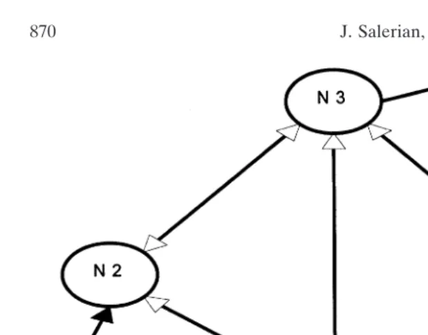
Figure 1. Possible structure of the hypothetical electricity market.
4. STRUCTURE OF AN ELECTRICITY MARKET
A hypothetical market is used in this study. It has the possibility of four nodes, which can be connected as shown in Figure 1.
Demand for electricity takes place at nodes N1 and N3. Genera-tion can take place at nodes N1, N2, and N4.
The aim is to determine the quantities of electricity consumed at nodes N1 and N3 and the location and capacity of transmission lines and power stations, which result in an economically efficient market, representing a long-run competitive equilibrium.
5. DEMAND
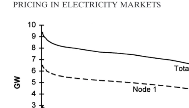
For each node where demand takes place, the load duration curve provides a useful description of demand across the year (see Figure 2).
Figure 2. Load duration curve for nodes N1 and N3.
is an additional complexity introduced because the demands at each node must be for the same points in time.
To ensure that the demands at each node are coincident in time, the following procedure is used. First, the load duration curve for one node (N1) was derived in the manner described above. Second, the load duration curve for the second demand node was determined using the chronological order of loads from the load duration curve at N1. This method was chosen for conve-nience. However, the method introduces some averaging issues into load duration curves of nodes other than the base node, N1. This means that the shape of the implied load duration curve for N3 may differ from that of its actual load duration curve. It would be useful to investigate the effects of any bias and consider alterna-tive methods for determining load blocks.
Thirty-four demand periods are defined by dividing the load duration curve for the first node into 100-MW load intervals. This create load blocks of unequal duration, measured in hours.
Each of the 34 load blocks is assumed to have an independent linear demand function that relates the amount of electricity de-manded to its price, and is given by:
Price5a1wQuantity. (19)
The parameters of each demand function, a and w, are cali-brated using assumed prices, quantities, and an own-price elasticity
of demand,E. The parameters are given by:
a5Price (121/E) andw51/E* Price/Quantity (20)
The price-elasticity of demand is assumed to be20.3.
6. TRANSMISSION
The special feature of this model is the incorporation of power flow equations into a meshed network. The presentation here is based on that of Chao and Peck (1996). The real power flow in a network, based on Kirchoff’s laws, is given by:
Qij5GijV2ij2GijViVjcos(ui2 uj)1YijViVjsin(ui2 uj) (21)
whereQis the power flow (measured in Gigawatts) from nodei
to node j, G, V, and Y are parameters relating to resistance,
voltage, and admittance.5uis the voltage phase angle at each node
(measured in radians). It is the difference in phase angles between two nodes that determines the magnitude of the power flow be-tween two nodes (see Chao and Peck, 1996, p. 35). The voltage phase angle and the power flow can be negatively valued. When
the power flow forQijis negative, the flow is from nodejto node
i. The transmission loss along the line is given by Qij 1Qji.
Under normal operating conditions, the real power flow equa-tions can be approximated by the following quadratic function (see Chao and Peck, 1996, p. 36, pp. 41–42, and pp. 50–52):
Qij5Gij(V2ij2ViVj)1YijViVj(ui2 uj)11/2GijViVj(ui2 uj)2fori,j (22)
In this power-flow equation, marginal power flow increases at a decreasing rate with respect to the phase angle and the function is convex.
Each of the nodes are connected by corridors made up of a number of transmission lines. The assumed technical properties of the transmission lines and the assumed maximum transmission capacities along the lines are described in Table 1.
The distance between nodes plays an important role in de-termining the overall characteristics of the line. For example,
5G
IN
E
LECTRICITY
MARKETS
[image:15.612.68.574.165.277.2]873
Table 1: Characteristics of the Network
Transmission lines
Link Resistance Impedance Construction
capacity Distance Voltage per km per km cost Life (MW) (km) No (kV) (V/km) (V/km) ($’000/km) (years)
N1–N2 2 500 25 5 33 0.03 0.3 383 50
N1–N3 1 875 150 5 50 0.025 0.25 391 50
N1–N4 3 750 150 5 33 0.03 0.3 389 50
N2–N3 3 000 160 5 33 0.03 0.3 383 50
Table 2: Plant Data
Maximum allowable
Power capacity Fuel cost Capacity Life Node station Availability MW $-MWh $m-MW Years
Node 1 P1 1 1 270 14.8 1.2 30
P2 1 861 14.3 1.4 30
P3 1 2 540 14.0 1.3 30
P4 1 500 18.5 1.2 30
Node 2 P5 1 unlimited 32 0.5 30
P6 1 unlimited 23.5 0.85 25
P4 1 500 18.5 1.2 30
P12 1 500 18.5 0.8 30
Node 4 P8 1 1 268 12.1 1.45 30
P9 1 960 13.0 1.3 30
P10 1 1 268 12.2 1.4 30
P11 1 890 14.8 1.25 30
although the same type of line can connect nodes N2–N3 and nodes N1–N2, the overall characteristics of the line vary significantly. In particular, the total resistance along a line N2–N3 is 6.4 times as great as between N1–N2, because the distance between N1–N3 is 6.4 times as large as N1.
7. PRODUCTION MODEL
The data for the power stations located at each node are shown in Table 2. There are several types of plants available, ranging from baseload (coal) through to peaking (gas).
8. RESULTS AND DISCUSSION
In this section, the physical and quantity variables are presented first, followed by price, revenue, and cost results.
8A. Results in Summary
Figure 3 summarizes the optimal solution of the numerical model. It shows the loading of power stations in each time block, the number of power lines on each link, and the direction of power flows in each block.
Figure 3. Optimal transmission structure, power flows, and loading.
but at the optimum, only three are built, all of which run at maximum capacity over all time blocks. Three power stations are built at node 1. Two of these stations (P3 and P2) provide baseload capacity, and the third (P1) provides intermediate and peaking capacity. Node 2 has four power stations that provide intermediate and peaking capacity.
8B. Demand
Figure 4. Load at demand nodes (GW).
capacity installed, this profit margin is generated by rationing demand so that price exceeds short-run marginal cost. This is analogous (in proposed electricity markets) to setting price equal to the value of foregone load when generating capacity is limiting. In the original load data (Figure 2), prices to consumers did not vary as much by load block, particularly in the extreme peak periods; this allowed demand to rise above the levels result-ing here.
8C. Generation by Location
Figures 5, 6, and 7 show the installed capacity and merit order dispatch of power stations located at three nodes in the network. It follows the expected pattern. The point raised in the previous section is evident here. Installed capacity reached a maximum well before the extreme peak period.
8D. Network Flows
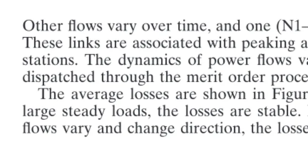
The average power flow for each link over time is shown in Figure 8. A negative number indicates that the direction of flow is the reverse of that implied in the name. For example, for link N1–N4, the flow is from N4 to N1.
Figure 5. Merit order generation at node 2.
Other flows vary over time, and one (N1–N2) reverses direction. These links are associated with peaking and intermediate power stations. The dynamics of power flows vary as these plants are dispatched through the merit order process.
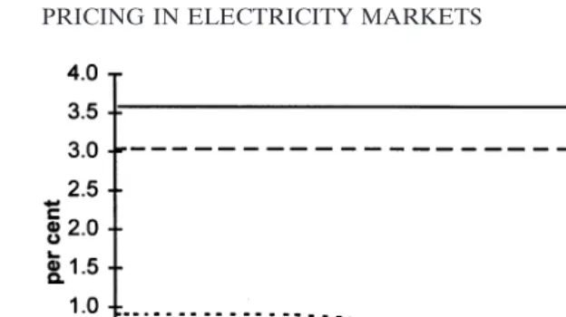
The average losses are shown in Figure 9. For the lines with large steady loads, the losses are stable. For lines where power flows vary and change direction, the losses vary over time.
[image:19.612.57.363.399.564.2]Figure 7. Merit order generation at node 4.
8E. Prices
As expected, the nodal prices are high in peak-load periods and low in base-load periods (Figure 10).
An interesting feature occurs at the very peak demand periods. Here, the welfare optimizing solution involves rationing demand rather than increasing the capacity of plants to satisfy very high
[image:20.612.57.365.399.566.2]Figure 9. Losses as a percentage of power flows.
demands for relatively short periods of duration. Consequently, at the very peak demands prices increase even further.
There are some periods of time when relatively large differences emerge between nodal prices.
The variation between nodal prices arising from capacity con-straints on transmission and the peak load-type cost recovery of
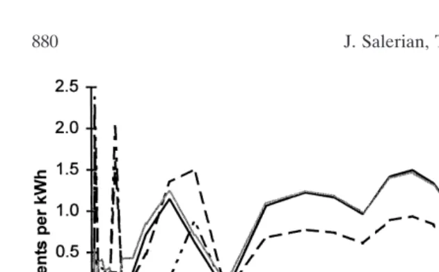
[image:21.612.58.366.386.560.2]Figure 11. Transmission prices by link.
transmission costs are evident in Figure 11. Transmission prices are calculated as the revenue from buying and selling electricity over the link in each time period divided by the average quantity of power flow over the link during each period. This is the average
merchandising surplus6per unit of power.
At some points in time, the transmission price is negative. This is the case referred to by Wu et al. (1996, p. 17), whereby economic dispatch can require power to flow from a node with a high price to one with a low price. In the presence of a transmission constraint and with Kirchoff’s laws in operation, it is welfare maximizing and economically efficient for one link to make a loss at a point in time. This is because the change in power flow allows the genera-tion and transmission of a lower cost source of electricity than could be obtained otherwise, resulting in net economic benefits.
8F. Sales Revenue
The revenue from sales to customers in each load block is shown in Table 3. This revenue is defined as the nodal price times the quantity sold. This is derived from the Kuhn-Tucker condition in Equation 11, in which total revenue is the nodal price times the quantity demanded, based on the linear demand functions.
Table 3: Revenue from Sales to Customers, by Node and Load Block ($Million)
Node
Load block N1 N3 Total
B1 32.26 15.89 48.15
B2 10.23 4.79 15.02
B3 17.80 8.45 26.26
B4 22.54 11.07 33.61
B5 38.32 18.90 57.22
B6 26.89 13.13 40.01
B7 40.10 19.71 59.80
B8 52.21 24.02 76.22
B9 49.37 24.84 74.21
B10 65.43 33.21 98.64
B11 78.63 43.32 121.95
B12 118.94 71.62 190.56
B13 104.56 58.89 163.45
B14 103.28 50.59 153.87
B15 114.35 76.63 190.98
B16 106.53 74.41 180.94
B17 80.09 54.64 134.73
B18 60.31 41.58 101.89
B19 46.75 39.84 86.59
B20 37.65 32.89 70.55
B21 29.28 25.96 55.23
B22 27.42 21.95 49.37
B23 26.32 20.74 47.06
B24 26.15 20.53 46.68
B25 26.69 17.05 43.74
B26 15.12 7.40 22.52
B27 19.21 9.45 28.65
B28 14.06 6.85 20.90
B29 13.52 6.59 20.11
B30 16.44 7.93 24.36
B31 12.50 6.05 18.55
B32 8.54 4.14 12.68
B33 6.17 3.01 9.18
B34 4.42 2.16 6.58
Total 1452.05 878.23 2330.28
As will be shown, the revenue from sales to customers is ulti-mately paid to the transmission network and generators.
8G. Transmission Revenue and Cost
Table 4 shows the revenue paid to each link of the transmission network.
This revenue is referred to as merchandising surplus by Wu et al. (1996) and Chao and Peck (1996). It is the difference between the revenue from sales (exports from the network) and the cost of energy imported (injected) into the network. For both the entire network and each link, the revenue received is equal to the total cost of transmission (including any rents arising from the number of lines on the link being constrained). This is a zero profit condi-tion on the network and each link, and is based on the Kuhn-Tucker conditions in Equation 18.
A point to note is that some nodes received negative revenue in some periods (load blocks). This situation arises when power flows along a line from a node with high price to one with a lower price. The reason this occurs is because of the externality arising from the power flow equations (based on Kirchoff’s laws) when there are transmission capacity constraints. For instance, the flow of power from node 2 to node 1, node 1 to node 4, and node 1 to node 3 enables more power to flow from node 2 to node 4. These power transfers help alleviate the congestion between node 2 and node 3. This enables consumers to source lower cost electric-ity, with some of the savings used to offset the loss on the power flows that made it possible.
8H. Generation Revenue and Costs
The revenues received for total generation at each node in each load block are shown in Table 5. The grand total for all nodes is 2144.35. This result is based on the second Kuhn-Tucker condition in Equation 12, where the revenue received at the node for local generation is equal to the revenue paid for local generation.
The revenue received at each node is then paid to the individual generators that produce power at each node in each load block, as shown in Table 6.
This revenue is the product of the nodal price and the output of each plant in each load period. This result is embedded in the second Kuhn-Tucker condition in Equation 13.
Table 4: Revenue Received by the Transmission Network and Transmission Cost ($Million)
Revenue received by each link
Total N1–N2 N1–N3 N1–N4 N2–N3 N3–N4 revenue
Load block
B1 0.01 0.08 0.44 0.06 0.03 0.61
B2 0.20 20.13 0.15 0.25 0.00 0.47
B3 0.25 20.15 0.25 0.32 0.00 0.68
B4 0.01 0.04 0.31 0.04 0.02 0.41
B5 0.01 0.11 0.52 0.07 0.03 0.74
B6 0.08 20.01 0.37 0.13 0.02 0.59
B7 0.01 0.07 0.55 0.06 0.03 0.73
B8 1.38 20.92 0.77 1.71 20.03 2.90
B9 20.03 0.44 0.65 0.20 0.06 1.33
B10 20.06 0.76 0.85 0.32 0.10 1.97
B11 20.34 3.02 0.90 1.11 0.27 4.96
B12 0.50 8.33 1.15 5.37 0.67 16.02
B13 2.31 4.81 1.15 6.35 0.41 15.04
B14 0.04 0.17 1.69 0.15 0.10 2.15
B15 21.40 13.16 0.83 4.35 1.01 17.95
B16 21.21 14.72 0.66 4.44 1.12 19.73
B17 20.60 10.67 0.55 2.92 0.81 14.35
B18 20.44 8.37 0.40 2.26 0.64 11.22
B19 20.52 11.70 0.01 3.03 0.86 15.09
B20 20.21 10.32 20.03 2.41 0.76 13.25
B21 20.01 8.52 20.05 1.82 0.63 10.91
B22 0.05 6.27 0.07 1.28 0.47 8.13
B23 0.26 6.13 0.07 1.04 0.46 7.95
B24 0.43 6.24 0.07 0.89 0.46 8.10
B25 0.26 3.26 0.27 0.43 0.25 4.46
B26 0.00 0.03 0.82 0.00 0.04 0.90
B27 0.00 0.03 1.10 0.00 0.06 1.19
B28 0.00 0.02 0.83 0.00 0.04 0.90
B29 0.00 0.02 0.83 0.00 0.04 0.89
B30 0.00 0.03 0.69 0.00 0.04 0.75
B31 0.00 0.02 0.54 0.00 0.03 0.59
B32 0.00 0.01 0.38 0.00 0.02 0.42
B33 0.00 0.01 0.29 0.00 0.01 0.32
B34 0.00 0.01 0.23 0.00 0.01 0.25
Total revenue 1.00 116.16 18.28 41.02 9.47 185.93
Transmission costs
Table 5: Revenue Received for Energy Produced at Each Node, by Load Block ($Million)
Load block N1 N2 N4 Total
B1 24.21 8.62 14.71 47.54
B2 7.68 2.22 4.65 14.55
B3 13.37 4.11 8.11 25.58
B4 16.92 6.01 10.27 33.20
B5 28.76 10.24 17.47 56.47
B6 20.18 6.99 12.25 39.43
B7 30.10 10.70 18.28 59.08
B8 39.19 10.40 23.74 73.32
B9 37.06 13.30 22.53 72.88
B10 49.12 17.68 29.87 96.67
B11 59.02 21.95 36.02 117.00
B12 89.28 30.55 54.71 174.54
B13 78.49 21.98 47.94 148.41
B14 77.50 27.46 46.77 151.73
B15 87.12 32.22 53.69 173.03
B16 82.89 27.09 51.22 161.21
B17 63.72 17.33 39.34 120.38
B18 48.14 12.80 29.73 90.67
B19 37.60 10.36 23.54 71.51
B20 30.95 6.94 19.42 57.30
B21 24.48 4.47 15.38 44.33
B22 23.04 3.59 14.61 41.24
B23 22.85 1.85 14.42 39.11
B24 23.27 0.52 14.79 38.58
B25 23.94 15.34 39.28
B26 13.36 8.26 21.62
B27 16.39 11.07 27.46
B28 11.66 8.34 20.01
B29 10.87 8.34 19.21
B30 12.80 10.81 23.61
B31 9.45 8.51 17.96
B32 6.22 6.04 12.26
B33 4.27 4.59 8.86
B34 2.76 3.57 6.33
Total 1126.65 309.37 708.32 2144.35
IN
E
LECTRICITY
MARKETS
[image:27.612.72.582.75.353.2]885
Table 6: Revenue Received by Each Power Station, in Each Load Block ($Million)
Load
block P1 P2 P3 P4 P5 P6 P8 P9 P11 P12 Total
B1 6.58 4.46 13.17 0.74 3.09 2.21 3.85 4.68 6.18 2.58 47.54 B2 2.09 1.42 4.17 0.19 0.80 0.57 1.22 1.48 1.96 0.66 14.55 B3 3.63 2.46 7.27 0.35 1.47 1.05 2.12 2.58 3.41 1.23 25.58 B4 4.60 3.12 9.20 0.52 2.16 1.54 2.69 3.27 4.32 1.80 33.20 B5 7.82 5.30 15.64 0.88 3.67 2.63 4.57 5.56 7.34 3.06 56.47 B6 5.49 3.72 10.97 0.60 2.51 1.79 3.20 3.90 5.15 2.09 39.43 B7 8.18 5.55 16.37 0.92 3.84 2.74 4.78 5.82 7.68 3.20 59.08 B8 10.66 7.22 21.31 0.89 3.73 2.67 6.21 7.55 9.98 3.11 73.32 B9 10.08 6.83 20.15 1.14 4.77 3.41 5.89 7.17 9.47 3.98 72.88 B10 13.35 9.05 26.71 1.52 6.34 4.53 7.81 9.50 12.55 5.29 96.67 B11 16.05 10.88 32.10 1.89 7.88 5.63 9.42 11.46 15.14 6.56 117.00 B12 24.27 16.46 48.55 2.62 10.96 7.83 14.31 17.41 22.99 9.13 174.54 B13 21.34 14.47 42.68 1.89 7.88 5.63 12.54 15.26 20.15 6.57 148.41 B14 21.07 14.29 42.14 2.37 9.78 7.07 12.23 14.88 19.66 8.24 151.73 B15 23.69 16.06 47.37 3.04 9.55 9.06 14.04 17.08 22.57 10.57 173.03 B16 22.54 15.28 45.08 2.96 5.02 8.82 13.40 16.30 21.53 10.29 161.21 B17 17.32 11.75 34.65 2.26 0.47 6.74 10.29 12.52 16.53 7.86 120.38 B18 13.09 8.87 26.18 1.71 5.12 7.78 9.46 12.50 5.97 90.67 B19 10.22 6.93 20.45 1.49 3.69 6.16 7.49 9.89 5.18 71.51 B20 8.41 5.70 16.83 1.25 1.35 5.08 6.18 8.16 4.34 57.30 B21 6.66 4.51 13.31 1.00 4.02 4.89 6.46 3.47 44.33 B22 5.98 4.32 12.74 0.46 3.82 4.65 6.14 3.14 41.24
B23 6.00 4.26 12.58 3.77 4.59 6.06 1.85 39.11
B24 5.99 4.37 12.90 3.87 4.70 6.21 0.52 38.58
J.
Salerian,
T.
Gregan,
and
A.
[image:28.612.69.571.148.295.2]Stevens
Table 6: Continued
Load
block P1 P2 P3 P4 P5 P6 P8 P9 P11 P12 Total
B25 5.79 4.60 13.56 4.01 4.88 6.44 39.28
B26 2.75 2.69 7.92 2.16 2.63 3.47 21.62
B27 2.17 3.60 10.62 2.90 3.52 4.66 27.46
B28 0.95 2.71 8.00 2.18 2.65 3.51 20.01
B29 0.15 2.71 8.00 2.18 2.65 3.51 19.21
B30 3.40 9.40 2.83 3.43 4.55 23.61
B31 2.67 6.77 2.23 2.70 3.58 17.96
B32 1.90 4.32 1.58 1.91 2.54 12.26
B33 1.44 2.83 1.20 1.45 1.93 8.86
B34 1.12 1.64 0.94 1.13 1.50 6.33
IN
E
LECTRICITY
MARKETS
[image:29.612.73.580.76.354.2]887
Table 7: Total Operating Cost for Each Power Station, by Load Block ($Million)
Load
block P1 P2 P3 P4 P5 P6 P8 P9 P10 P12
B1 0.69 0.45 1.34 0.10 0.71 0.37 0.35 0.46 0.57 0.34 B2 0.25 0.16 0.47 0.03 0.25 0.13 0.12 0.16 0.20 0.12 B3 0.45 0.29 0.87 0.06 0.46 0.24 0.23 0.30 0.37 0.22 B4 0.61 0.39 1.18 0.09 0.63 0.33 0.31 0.41 0.50 0.30 B5 1.10 0.71 2.13 0.16 1.13 0.59 0.56 0.73 0.91 0.54 B6 0.86 0.55 1.66 0.12 0.88 0.46 0.44 0.57 0.71 0.42 B7 1.39 0.89 2.68 0.20 1.42 0.74 0.71 0.92 1.14 0.68 B8 1.96 1.26 3.79 0.28 2.00 1.05 1.00 1.30 1.61 0.96 B9 2.04 1.31 3.95 0.29 2.09 1.09 1.04 1.36 1.68 1.00 B10 3.06 1.96 5.92 0.43 3.13 1.64 1.56 2.03 2.52 1.51 B11 4.21 2.70 8.13 0.59 4.30 2.26 2.14 2.79 3.46 2.07 B12 7.27 4.66 14.05 1.03 7.43 3.90 3.69 4.83 5.98 3.58 B13 7.72 4.95 14.91 1.09 7.88 4.14 3.92 5.12 6.35 3.80 B14 9.68 6.21 18.70 1.37 9.78 5.19 4.92 6.43 7.97 4.76 B15 12.41 7.96 23.99 1.76 9.55 6.66 6.31 8.24 10.22 6.11 B16 12.09 7.75 23.36 1.71 5.02 6.48 6.14 8.03 9.95 5.95 B17 9.23 5.92 17.83 1.30 0.47 4.95 4.69 6.13 7.60 4.54 B18 8.74 5.60 16.89 1.24 4.69 4.44 5.80 7.19 4.30 B19 8.29 5.32 16.02 1.17 3.69 4.21 5.50 6.82 4.08 B20 6.94 4.45 13.42 0.98 1.35 3.53 4.61 5.71 3.42
B21 6.41 4.11 12.39 0.91 3.26 4.26 5.28 3.16
B22 5.98 4.09 12.31 0.46 3.24 4.23 5.24 3.14
B23 6.00 4.03 12.15 3.19 4.18 5.18 1.85
B24 5.99 4.14 12.47 3.28 4.28 5.31 0.52
J.
Salerian,
T.
Gregan,
and
A.
[image:30.612.68.570.149.295.2]Stevens
Table 7: Continued
Load
block P1 P2 P3 P4 P5 P6 P8 P9 P10 P12
B25 5.79 4.35 13.10 3.44 4.50 5.58
B26 2.75 2.54 7.65 2.01 2.63 3.26
B27 2.17 3.40 10.26 2.70 3.52 4.37
B28 0.95 2.57 7.73 2.03 2.65 3.29
B29 0.15 2.57 7.73 2.03 2.65 3.29
B30 3.33 9.40 2.63 3.43 4.27
B31 2.62 6.77 2.07 2.70 3.36
B32 1.86 4.32 1.47 1.91 2.39
B33 1.41 2.83 1.12 1.45 1.81
B34 1.10 1.64 0.87 1.13 1.41
IN
E
LECTRICITY
MARKETS
[image:31.612.70.584.77.352.2]889
Table 8: Gross Margin for Each Power Station, by Load Block ($Million)
Load
block P1 P2 P3 P4 P5 P6 P8 P9 P10 P12 Total
B1 5.89 4.02 11.83 0.64 2.38 1.84 3.49 4.22 5.61 2.23 42.15 B2 1.84 1.26 3.70 0.16 0.55 0.44 1.09 1.32 1.75 0.54 12.65 B3 3.18 2.18 6.40 0.29 1.02 0.81 1.89 2.28 3.04 1.01 22.09 B4 3.99 2.73 8.02 0.43 1.53 1.21 2.38 2.86 3.81 1.50 28.45 B5 6.72 4.59 13.51 0.72 2.55 2.03 4.01 4.83 6.43 2.52 47.92 B6 4.63 3.17 9.32 0.48 1.63 1.33 2.77 3.33 4.44 1.67 32.77 B7 6.79 4.66 13.68 0.72 2.42 2.00 4.08 4.89 6.54 2.52 48.31 B8 8.69 5.97 17.52 0.62 1.73 1.61 5.21 6.25 8.36 2.14 58.11 B9 8.03 5.52 16.21 0.85 2.68 2.31 4.85 5.81 7.79 2.97 57.04 B10 10.29 7.09 20.79 1.09 3.22 2.89 6.26 7.47 10.03 3.78 72.90 B11 11.84 8.18 23.97 1.29 3.58 3.37 7.28 8.67 11.68 4.49 84.36 B12 17.01 11.80 34.50 1.60 3.53 3.94 10.62 12.58 17.01 5.56 118.13 B13 13.62 9.52 27.76 0.80 1.50 8.62 10.13 13.80 2.77 88.51 B14 11.39 8.08 23.44 1.00 1.88 7.32 8.46 11.69 3.48 76.73 B15 11.27 8.10 23.38 1.28 2.41 7.74 8.84 12.35 4.46 79.82 B16 10.45 7.53 21.72 1.25 2.34 7.26 8.27 11.58 4.34 74.74 B17 8.10 5.83 16.82 0.95 1.79 5.60 6.39 8.94 3.31 57.72 B18 4.35 3.27 9.29 0.48 0.43 3.34 3.66 5.30 1.67 31.78 B19 1.93 1.61 4.43 0.32 1.95 1.99 3.07 1.10 16.40 B20 1.47 1.25 3.41 0.27 1.55 1.57 2.45 0.92 12.89
B21 0.24 0.40 0.92 0.09 0.77 0.64 1.19 0.32 4.56
B22 0.23 0.43 0.58 0.42 0.90 2.56
B23 0.23 0.42 0.58 0.41 0.88 2.52
B24 0.24 0.44 0.59 0.42 0.90 2.59
J.
Salerian,
T.
Gregan,
and
A.
[image:32.612.69.573.149.295.2]Stevens
Table 8: Continued
Load
block P1 P2 P3 P4 P5 P6 P8 P9 P10 P12 Total
B25 0.25 0.46 0.57 0.38 0.87 2.52
B26 0.15 0.27 0.15 0.21 0.78
B27 0.19 0.36 0.20 0.29 1.04
B28 0.15 0.27 0.15 0.22 0.78
B29 0.15 0.27 0.15 0.22 0.78
B30 0.07 0.20 0.28 0.55
B31 0.06 0.15 0.22 0.43
B32 0.04 0.11 0.16 0.31
B33 0.03 0.08 0.12 0.23
B34 0.02 0.06 0.09 0.18
Table 9: Summary of Power Station Revenue and Costs ($Million)
Total Total Construction Plant revenue variable cost1 costs2 capacity rents3
P1 286.93 135.19 135.37 16.37
P2 214.14 105.59 107.07 1.47
P3 625.58 312.05 293.31 20.22
P4 30.67 15.36 15.31
P5 83.94 57.12 26.65 0.17
P6 84.09 49.95 34.15
P8 185.27 83.64 101.63
P9 225.33 109.25 110.86 5.22
P10 297.72 135.51 157.69 4.52
P12 110.68 57.38 35.53 17.77
1Total variable costs that include fuel costs and other variable costs of running power station.
2Construction costs that are equal to the annualized cost of building the power station of the capacity installed.
3Plant capacity rents are the rents accruing because the installed capacity of the power station is at the maximum allowed.
Table 9 shows that the revenue received by each power station is equal to total variable cost plus construction costs and plant capacity rents. It shows that there are zero profits. The plant capacity rents represent the opportunity cost of the limit on in-stalled capacity of the particular power station. Together, Kuhn-Tucker conditions in Equation 13 and 14 determine these results.
9. CONCLUSION AND FURTHER RESEARCH
The model presented here provides insights into economic is-sues arising in electricity markets. It has integrated demand, trans-mission, and generation into a single model to simulate the eco-nomically efficient operation of an electricity market.
The pricing rules embodied in this long-run model allow nodal and transmission prices to be optimized over time and space. In this model, the costs of generation and transmission are fully re-covered.
The approach used here contrasts with other models of transmis-sion pricing where losses play a key role in determining nodal prices and Kirchoff’s laws are omitted.
This model provides a framework against which to assess other approaches to transmission pricing, such as Backerman, Rassenti, and Smith (1996), and the approach being proposed by the Austra-lian National Electricity Code (NEMMCO, 1996).
Future research could use the framework in this paper to com-pare the models of transmission pricing arrangements being pro-posed for access pricing to electricity network in deregulated elec-tricity markets.
REFERENCES
Backerman, S.R., Rasseneti, S.J., and Smith, V.L. (1996) Efficiency and Income Shares in High Demand Energy Networks: Who Receives the Congestion Rents When a Line Is Constrained? (mimeo) Tuscon, AZ: Economic Science Laboratory, The University of Arizona.
Balinski, M.L., and Baumol, W.J. (1968) The Dual in Nonlinear Programming and its Economic Interpretation.Review of Economic Studies35:237–256.
Bisschop, J., and Meeraus, A. (1982) On the Development of a General Algebraic Model-ling System.A Strategic Planning Environment, Mathematical Programming Study 20:1–29.
Brooke, A., Kendrick, D., and Meeraus, A. (1992)GAMS: A User’s Guide.Release 2.25. Denver, MA: Boyd and Fraser Publishing Company.
Bushnell, J.B., and Stoft, S. (1996) Electric Grid Investment Under a Contract Network Regime.Journal of Regulatory Economics10:61–79.
Chao, H., and Peck, S. (1996) A Market Mechanism For Electric Power Transmission. Journal of Regulatory Economics10:25–59.
Dalziell, I., Noble, K., and Ofei-Mensah, A. (1993)The Economics of Interconnection: Electricity Grids and Gas Pipelines in Australia.ABARE Research Report 93.12. Canberra: Australian Bureau of Agricultural and Resource Economics.
Hobbs, B.F., and Schuler, R.E. (1985) Evaluation of Electric Power Deregulation Using Network Models of Oligopolistic Spatial Markets. In Spatial Price Equilibrium: Advances in Theory, Computation and Application (P.T. Harker, Ed.). Berlin: Springer Verlag, pp. 208–254.
Kolstad, C.D. (1989) Computing Dynamic Spatial Oligopolistic Equilibria in an Exhaustible Resource Market. InQuantitative Methods for Market Oriented Economic Analysis over Space and Time(W.C. Labys, T. Takayama, and N.D. Uri, Eds.). Harts, UK: Gower Publishing Company Limited.
MacAulay, T. (1992) Alternative Spatial Equilibrium Formulations: A Synthesis. In Contri-butions to Economic Analysis(J. Tinbergen, D. Jorgenson, and J. Laffont, Eds.). Amsterdam: North-Holland Publishing Company.
Munasinghe, M. (1990)Electric Power Economics.London: Butterworths & Co. NEMMCO (National Electricity Market Management Company) (1996)National
Electric-ity Code.Draft Version 2.0, October. Melbourne: NEMMCO. http://www.nemmco. com.au/codeinfo.htm
Provenzano, G. (1989) Alternative National Policies and the Location Patterns of Energy Related Facilities. InQuantitative Methods for Market Oriented Economic Analysis over Space and Time(W.C. Labys, T. Takayama, and N.D. Uri, Eds.). Harts, UK: Gower Publishing Company Limited.
Salerian, J.S. (1992) The Application of a Temporal Price Allocation Model to Time-of-Use Electricity Pricing. Discussion Paper 92.11, Department of Economics, University of Western Australia, Nedlands, Western Australia.
Samuelson, P.A. (1952) Spatial Price Equilibrium and Linear Programming.American Economic Review42:283–303.
Scherer, C.R. (1977) Estimating Electric Power System Marginal Costs. In Contributions to Economic Analysis (vol. 107). Amsterdam: North-Holland Publishing Company. Sohl, J.E. (1985) An Application of Quadratic Programming to the Deregulation of Natural Gas. InSpatial Price Equilibrium: Advances in Theory, Computation and Application (P.T. Harker, Ed.). Berlin: Springer Verlag. pp. 198–207.
Stocks, K., and Musgrove, A. (1984) MENSA—Regionalised Version of MARKAL: The IEA Linear Programming Model for Energy Systems Analysis.Energy Systems and Policy4:313–348.
Takayama, T., and Judge G.G. (1971)Spatial and Temporal Price and Allocation Models. Amsterdam: North-Holland Publishing Company.
Takayama, T., and Woodland, A.D. (1970) Equivalence of Price and Quantity Formulations of Spatial Equilibrium: Purified Duality in Quadratic and Concave Programming. Econometrica38:899–906.
Turvey, R., and Anderson, D. (1977)Electricity Economics, Essays and Case Studies. Baltimore: The Johns Hopkins University Press.
Uri, N.D. (1983)New Dimensions in Utility Pricing. London, UK: JAI Press Inc. Uri, N.D. (1989) Linear Complementary Programming. Electrical Energy as a Case Study.
InQuantitative Methods for Market Oriented Economic Analysis over Space and Time(W.C. Labys, T. Takayama, and N.D. Uri, Eds.). Harts, UK: Gower Publishing Company Limited.