Electronic Journal of Qualitative Theory of Differential Equations 2003, No. 15, 1-19;http://www.math.u-szeged.hu/ejqtde/
On the structure of spectra of travelling waves
Peter L. Simon
Department of Applied Analysis,
E¨
otv¨
os Lor´
and University Budapest, Hungary
E-mail: [email protected]
October 19, 2003
Abstract
The linear stability of the travelling wave solutions of a general reaction-diffusion system is in-vestigated. The spectrum of the corresponding second order differential operatorLis studied. The problem is reduced to an asymptotically autonomous first order linear system. The relation between the spectrum of L and the corresponding first order system is dealt with in detail. The first order system is investigated using exponential dichotomies. A self-contained short presentation is shown for the study of the spectrum, with elementary proofs. An algorithm is given for the determination of the exact position of the essential spectrum. The Evans function method for determining the isolated eigenvalues ofL is also presented. The theory is illustrated by three examples: a single travelling wave equation, a three variable combustion model and the generalized KdV equation.
Keywords: linear stability of travelling waves, exponential dichotomies, Evans function
AMS classification: 35K57, 35B32.
1
Introduction
We investigate the stability of the travelling wave solutions of the system
∂τu=D∂xxu+f(u), (1)
where u : R+×R → Rm, D is a diagonal matrix with positive diagonal elements andf : Rm → Rm
is a continuously differentiable function. The travelling wave solution of this equation has the form
u(τ, x) =U(x−cτ), where U :R→Rm. For this function we have
DU′′(z) +cU′(z) +f(U(z)) = 0, (z=x−cτ) (2)
The stability ofU can be determined by linearization. Puttingu(τ, x) =U(x−cτ) +v(τ, x−cτ) in (1) the linearized equation forv takes the form
∂τv=D∂zzv+c∂zv+f′(U(z))v. (3)
According to well known stability theorems (see e.g. [21]) the stability of the travelling wave solutionU
is determined by the spectrum of the second order differential operator
(LV)(t) =DV′′(t) +cV′(t) +Q(t)V(t), (4)
defined inC0(R,Cm)∩C2(R,Cm), whereQ(t) =f′(U(t)),
C0(R,Cm) ={V :R→Cm|V is continuous, lim
endowed with the supremum normkVk= maxR|V(t)|. It is assumed thatQ:R→Cm×mis continuous,
and the limitsQ±= lim
t→±∞Q(t) exist.
The complex numberλ∈Cis called a regular value ofLif the operatorL−λIhas bounded inverse that
is defined in the whole spaceC0(R,Cm). That is for anyW ∈C0(R,Cm) there exists a unique solution of
LV −λV =W in C0(R,Cm)∩C2(R,Cm), and there existsM >0 such that for anyW ∈C0(R,Cm) we
havekVk ≤MkWk. The spectrumσ(L) ofLconsists of non-regular values. The numberλis called an eigenvalue ifL−λI has no inverse. The essential spectrum ofLconsists of those points of the spectrum which are not isolated eigenvalues with finite multiplicity. It is useful to introduce the first order system corresponding to equationLV −λV =W. Letx= (V, V′)T,y= (0, W)T, then the first order system is
˙
x(t) =Aλ(t)x(t) +y(t), (5)
where
Aλ(t) =
0 I
D−1(λI−Q(t)) −cD−1
. (6)
The spectrum of L has been widely investigated. The position of the essential spectrum has been estimated, see e.g. [14], and Weyl’s lemma in [21]. This can be done using exponential dichotomies for the first order system (5), [5, 18]. This approach was also generalized to infinite dimensional systems, when A is a bounded operator on a Banach space [6] and also for unbounded operators [4]. Fredholm properties are also relevant when determining the spectrum ofL [11, 18]. The relation between these two concepts is dealt with in [16, 18]. The determination of the isolated eigenvalues requires to solve a linear system with non-constant coefficients, which can be done in general only numerically. For the investigation of the isolated eigenvalues two concepts were introduced. The first was the Evans function [10], which is an analytic function on the complex plane, the zeros of which are the isolated eigenvalues ofL. Later a topological invariant was introduced for the study of the spectrum [1]. These methods were applied for several systems in physics [3, 12, 17], chemistry [2, 7, 13, 19] and biology [10, 15].
The aim of the paper is to present a self-contained detailed study of the spectrum of L, and to fill the gap between the abstract results (on exponential dichotomies and on topological invariants) and the applications. The novelties of the paper are as follows.
• An algorithm is given for the determination of the exact position of the essential spectrum. The statements concerning the essential spectrum are proved by elementary methods. (Most of the known results give only sufficient conditions for the essential spectrum to lie in the left half plane.)
• All the theorems are proved in the finite dimensional case. The presentation does not need abstract techniques, hence for those applying the theory a self-contained method is shown. (According to the author’s knowledge a self-contained explanation, including the proofs, is only given for the case of unbounded operators [4]. The proof of the finite dimensional case must be compiled from different sources, e.g. [5, 8, 14, 16].)
• The relation between the spectrum of L and the corresponding first order system is dealt with in detail. (The standard reference in this context is [14] but the relation is not proved in that book.)
2
Relation between the spectrum of
L
and the first order system
Lemma 1 connects the determination of the spectrum of L with the study of system (5). In order to prove the lemma we will need the following Proposition.
Proposition 1 If W ∈ C0(R,Cm) and V ∈ C0(R,Cm) is the solution of LV −λV = W, then V′ ∈
C0(R,Cm).
ProofWe will show thatV′ →0 at +∞, it can be verified similarly, thatV′→0 at−∞. Let us denote
byz the real or imaginary part of the k-th coordinate ofV, (k is arbitrary), and letd=Dkk. We will
prove that limt→+∞z˙(t) = 0 that implies the desired statement. First we prove in the casec6= 0. Since
V andW tend to 0 at +∞, for anyε >0 there existst0 such that
Dividing bydand multiplying by exp (ct/d) we obtain
In the casec <0 we prove by contradiction. Assume that there existsα >0 and a sequencetn→ ∞,
such that|z˙(tn)|=α. Let ε=−cα/2 and apply (7) fort0 =tn whenn is large enough. If ˙z(tn) =α,
then the inequality in the left hand side of (7) yields fort > tn that
˙
ast→+∞. This contradicts to the boundedness ofz.
Finally, let us consider the casec= 0. Then from the differential equation we get that ¨ztends to zero at infinity. According to the Landau-Kolmogorov inequality (see e.g. [9])kz˙k ≤4k¨zkkzk. Definingk · k as the supremum norm on [T,+∞) forT large enough, we get that ˙z→0 at infinity.
such that for any y satisfying the above conditions the corresponding unique solution x satisfies
kxk ≤M(kyk+ky˙k).
The differentiability ofy1 implies that V is twice differentiable and ¨V = ˙U+ ˙y1, hence from the second equation
Since λ is a regular value of L, this equation has a unique solution V ∈ C0(R,Cm), and there exists
M1>0 for which
kVk ≤M1(ky˙1k+ky1k+ky2k). (8) Moreover, according to Proposition 1 ˙V ∈ C0(R,Cm), yielding U = ˙V −y1 ∈ C0(R,Cm). Thus x ∈
C0(R,C2m) what we wanted to prove.
Now we show the continuous dependence of x on y. Let us denote the maximum point of ˙Vk (for
somek= 1, . . . , m) bytk. Since ˙Vk→0 at±∞, the maximum point is not at infinity, hence ¨Vk(tk) = 0.
Therefore using (8) we get that there existsM2>0 for which
|V˙k(tk)| ≤M2(ky˙1k+ky1k+ky2k).
Similar inequality can be proved for the minimum of ˙Vk, and for all coordinates ofV, hence there exists
M3 >0 for which kV˙k ≤M3(ky˙1k+ky1k+ky2k). Since U = ˙V −y1, there existsM4 >0 for which kUk ≤M4(ky˙1k+ky1k+ky2k). Thus withM = 2(M1+M4) we havekxk ≤M(kyk+ky˙k).
Now we turn to the study of general first order systems, the special case of which is system (5).
3
First order systems
Now for short letC0=C0(R,Cn) endowed with the supremum normkxk= maxR|x(t)|, and letA:R→
Cn×n be a continuous function for which the limits
A± = lim
t→±∞A(t) exist. Let us consider the first order system
˙
x(t) =A(t)x(t) +y(t). (9)
Our aim is to give necessary and sufficient condition for the existence and uniqueness of a solutionx∈C0 of (9) for anyy∈C0, and for the continuous dependence ofxony.
SinceA is continuous, system (9) has solutions for anyy∈C0, that can be given by the variation of constants formula as
x(t) = Ψ(t)x0+
t
Z
0
Ψ(t)Ψ(s)−1y(s)ds, (10)
where Ψ is the fundamental system of solutions of the homogeneous equation satisfying Ψ(0) =I, i.e. thencolumns of the matrix Ψ(t) arenindependent solutions of the homogeneous system
˙
x(t) =A(t)x(t). (11)
Hence the question is that for a giveny∈C0 does there exist a uniquex0∈Cn, such thatx∈C0 (xis given by (10)), and that doesxdepend continuously ony.
The dimension of the stable, unstable and central subspaces of the matricesA± play important role. Let us denote the number of eigenvalues (with multiplicity) ofA+ with positive, negative, zero real part byn+
u,n+s, n+c, respectively. We definenu−,n−s,n−c similarly usingA−.
First we show that the continuous dependence is violated whenn+
c >0 orn−c >0. The main point
in these cases is to prove the existence of a bounded solution of the homogeneous equation, which does not tend to zero.
Theorem 1 Let us assume that at least one of the following two conditions holds:
(a) n+
c >0 and
R+∞
0 |A(t)−A +|<∞
(b) n−
c >0 and
R0
−∞|A(t)−A
−|<∞.
Then the solution of (9) does not depend continuously ony, in the sense that there is noM >0for which
ProofWe prove in case (a), the other case is similar. According to Theorem 1.10.1 of [8] there exists z0∈ Cn, such that the solution t7→Ψ(t)z0 of (11) is bounded in [0,+∞) but does not tend to zero as
t→+∞. Then there exista >0 and a sequencetk →+∞, such that|Ψ(tk)z0|=afor allk= 1,2, . . ..
Lethk :R→Rbe continuously differentiable functions satisfying the following conditions
hk|(−∞,0]= 0, |hk| ≤1, |h˙k| ≤1, tk Z
0
hk = 1,
+∞
Z
0
hk= 0, lim
+∞hk = 0 lim+∞ ˙
hk= 0.
Letyk(t) =hk(t)Ψ(t)z0, then yk∈C0,yk is differentiable and
˙
yk(t) = ˙hk(t)Ψ(t)z0+hk(t) ˙Ψ(t)z0= ˙hk(t)Ψ(t)z0+hk(t)A(t)Ψ(t)z0.
Hence ˙yk → 0 at +∞, since hk → 0, ˙hk → 0 and A(t) is bounded. On the other hand, there exists
M1>0 for whichky˙kk ≤M1 for allk= 1,2, . . .. Let
xk(t) = t
Z
0
Ψ(t)Ψ(s)−1y
k(s)ds
Thenxk is a solution of (9) belonging toyk, andxk(t) = Ψ(t)z0R
t
0hk(s)ds, hencexk∈C0. However, kxkk= max
t∈R |xk(t)| ≥ |xk(tk)|=tka.
Since kykk ≤ kΨ(·)z0k for all k = 1,2, . . ., the inequality kxkk ≤ M(kykk+ky˙kk) would meantka ≤
M(kΨ(·)z0k+M1) for all k= 1,2, . . ., which contradicts totk→+∞.
In the further considerations we will assume n+
c = 0 or n−c = 0. In this case we will use exponential
dichotomies to answer the above question.
Definition 1 System (11) possesses an exponential dichotomy in the intervalJ if there exist a projection
P and positive numbersK, L, α, β, such that
kΨ(t)PΨ(s)−1k ≤Ke−α(t−s) fort≥s, t, s∈J (12)
kΨ(t)(I−P)Ψ(s)−1k ≤Le−β(s−t) fors≥t, t, s∈J (13)
We will show that the exponential dichotomy on R implies the existence, uniqueness and continuous
dependence of the solution of (9). It can be shown that system (11) possesses an exponential dichotomy onRifA(t) is constant and it has no eigenvalues on the imaginary axis, that is whenn+c =n−c = 0. For
the time dependent case there is no exponential dichotomy onRin general whenn+c =n−c = 0. However,
we will show that system (11) possesses exponential dichotomies onR+and onR−. If the projections of
these two dichotomies are the same, then system (11) possesses an exponential dichotomy onRas well,
and the existence, uniqueness and continuous dependence follows. We will use the following properties of exponential dichotomies.
Lemma 2 (i) Let P1 and P2 be projections, for which ImP1 =ImP2. If system (11) possesses an
exponential dichotomy in the interval J with the projection P1, then it possesses an exponential
dichotomy in the interval J with the projectionP2 as well.
(ii) System (11) possesses an exponential dichotomy in any closed and bounded interval [a, b], with any
projection.
(iii) If system (11) possesses an exponential dichotomy in the intervals (a, b] and [b, c) with the same
projection P, then it possesses an exponential dichotomy in the interval (a, c)(here acan be−∞,
andc can be +∞).
Proof
(ii) The function (t, s)7→ kΨ(t)PΨ(s)−1keα(t−s)is continuous on the square [a, b]×[a, b], hence it has a maximumK, implying (12). Inequality (13) follows similarly.
(iii) We only have to prove that (12) holds for t ∈ [b, c), s ∈ (a, b], and that (13) holds for s ∈ [b, c),
t∈(a, b]. We will show only the first one, the proof of the second one is similar. Thus leta < s≤b≤t < c. Then
kΨ(t)PΨ(s)−1k=kΨ(t)PΨ(b)−1Ψ(b)PΨ(s)−1k ≤Ke−α(t−b)Ke−α(b−s)=K2e−α(t−s).
The following Lemma can be proved using the results in [5].
Lemma 3 (i) Ifn+
c = 0, then system (11) possesses an exponential dichotomy in[0,+∞), the
projec-tion of which is denoted byP+. Moreover, dim(kerP+) =n+
u,dim(ImP+) =n+s.
(ii) Ifn−
c = 0, then system (11) possesses an exponential dichotomy in(−∞,0], the projection of which
is denoted byP−. Moreover, dim(kerP−) =n−
u,dim(ImP−) =n−s.
ProofWe prove only (i), the second statement can be verified similarly. Sincen+
c = 0, system ˙x=A+x with constant coefficients possesses an exponential dichotomy in [0,+∞) the projection of which, denoted byP+, has ann+
s dimensional range andn+u dimensional kernel, see [5] pp.10. For anyδ >0 there exists
t0>0, such thatkA(t)−A+k< δfort > t0. Hence according to proposition 1 of [5] on pp. 34 system (11) possesses an exponential dichotomy in [t0,+∞) with projectionP+. Applying statements (ii) and (iii) of Lemma 2 we can complete the proof.
Let us introduce the following subspaces.
Es+= ImP+, Eu+= kerP+= Im (I−P+), Es−= ImP−, Eu−= kerP−= Im (I−P−).
According to the next Proposition the subspaceE+
s consists of those initial conditionsx0, for which the
solution of the homogeneous equation tend to 0 ast→+∞. Similarly, the subspaceE−
u consists of those
initial conditionsx0, for which the solution of the homogeneous equation tend to 0 ast→ −∞.
Proposition 2 (i) Assumen+
c = 0. Then limt→+∞Ψ(t)x0= 0 if and only ifx0∈Es+.
(ii) Assume n−
c = 0. Then limt→−∞Ψ(t)x0= 0if and only ifx0∈Eu−.
ProofWe prove only (i), the second statement can be verified similarly. Forx0∈E+
s we haveP+x0=x0, hence settings= 0 in (12)
|Ψ(t)x0| ≤Ke−αt|x0| t >0.
Thus forx0∈Es+ we have proved limt→+∞Ψ(t)x0= 0.
Let us assume now limt→+∞Ψ(t)x0= 0. Sincex0=P+x0+ (I−P+)x0 andP+x0∈Es+ we have
0 = lim
t→+∞Ψ(t)x0= limt→+∞Ψ(t)P +x
0+ lim
t→+∞Ψ(t)(I−P +)x
0= lim
t→+∞Ψ(t)(I−P +)x
0 (14)
Applying (13) to Ψ(s)(I−P+)x
0 and settingt= 0 we get
|(I−P+)x0|L−1eβs≤ |Ψ(s)(I−P+)x0| s >0.
Therefore (14) can be satisfied only in the case (I−P+)x
0 = 0, which means that x0 ∈Es+, what we
had to prove.
Corollary 1 Let us assume n+
c =n−c = 0. The homogeneous equation (11) has a unique solution inC0
(it isx≡0) if and only ifdim(E+
s ∩Eu−) = 0.
ProofLet us assume dim(E+
s ∩Eu−) = 0. If for a solution x= Ψ(·)x0 of (11) we have lim±∞x= 0, then according to Proposition 2x0∈Es+∩Eu−, hence x0= 0, that isx≡0.
Let us now assume dim(E+
s ∩Eu−)>0. Let x0 ∈Es+∩Eu−, x0 6= 0. Thenx= Ψ(·)x0 is a nonzero solution of (11) and lim±∞x= 0.
Lemma 4 Lety∈C0,x0∈Cn and letxbe given by (10).
Now we prove the convergence of the second term. Let ε > 0 be an arbitrary positive number. Since lim+∞y= 0, there existst1>0 such that, fort > t1 we have|y(t)|< εα/2K. Lett2> t1 be a number
Thus (17) is verified. Similarly we can prove
lim
Now we show that (15) is equivalent to
lim bounded function. Let us assume first that (15) holds. Then
According to (13)
Now let us assume that (19) holds. Let us introducex∗ by
(I−P+)x∗:=
We have seen that the second term tends to zero ast→+∞, hence
lim
t→+∞Ψ(t)(I−P +)(x
0+x∗) = 0
implyingx0+x∗= 0 according to Proposition 2, hencex0=−x∗, yielding (15). Similarly we can prove that (16) is equivalent to
lim
Now the proof of statement (i) of the Lemma follows from the equation
x(t) = Ψ(t)P+x0+ the sum of the third and fourth term tends to zero ast→+∞. According to (19) this sum tends to zero if and only if that (15) holds, what we had to prove.
The proof of statement (ii) of the Lemma follows similarly from (18) and (20).
Lemma 5 Let us assumen+
c =n−c = 0. The following two statements are equivalent.
(i) For any a∈E+
Let us assume that (i) holds. First we show thatE+
Now let us assume that (ii) holds. First we show that the solution in (i) is unique. Let us assume that there are two solutionsx′
0andx′′0. Introducingx0=x′0−x0′′we haveP−x0= 0 and (I−P+)x0= 0. Hence x0 ∈ Eu−∩Es+, yielding x0 = 0, that is x′0 = x′′0. Now we show that the solution x0 in (i) exists. Let z1 ∈ Es+, z2 ∈ Eu−, such that a−b = z1+z2 and let x0 = b+z2 = a−z1. Then (I−P+)x
0= (I−P+)(a−z1) =a, sinceP+a= 0 and (I−P+)z1= 0. SimilarlyP−x0=P−(b+z2) =b.
The following lemma is proved in [16] Prop. 2.1 and in [5] p. 19, but in order to make the paper self-contained we present a short proof.
Lemma 6 Let us assumen+
c =n−c = 0andEs+⊕E−u =Cn. Then system (11) possesses an exponential
dichotomy inRwith a projection P∗, for which ImP∗=E+
s,kerP∗=Eu−.
ProofAssumption E+
s ⊕Eu− =Cn implies that there exists a projection P∗, for which ImP∗ =Es+,
kerP∗=E−
u. Namely, for an arbitrary vectorz∈Cn we can defineP∗z asP∗z=z1, wherez=z1+z2 with z1 ∈ Es+, z2 ∈ Eu−. Since ImP∗ = ImP+, Lemma 2 and Lemma 3 imply that system (11)
possesses an exponential dichotomy in [0,+∞) with the projectionP∗. On the other hand Im (I−P∗) = Im (I−P−), hence Lemma 2 and Lemma 3 imply that system (11) possesses an exponential dichotomy in (−∞,0] with the projectionP∗. Since system (11) possesses an exponential dichotomy both in [0,+∞) and in (−∞,0] with the projectionP∗, according to Lemma 2 it possesses an exponential dichotomy in
R.
Theorem 2 Let us assumen+
c =n−c = 0.
(i) If for any differentiable functiony∈C0, for which y˙∈C0 there exists a unique solution x∈C0 of
(9), then E+
s ⊕Eu−=Cn.
(ii) If E+
s ⊕Eu− = Cn, then system (9) has a unique solution x ∈ C0 for any y ∈ C0, and there
exists M >0, such that for anyy ∈ C0 and for the corresponding solution x∈ C0 the inequality
kxk ≤Mkyk holds.
Proof(i) Let us assume that system (9) has a unique solution x∈ C0 for any differentiable function y∈C0, for which ˙y∈C0. Leta∈E+
u andb∈Es− be arbitrary vectors. We will show that there exists a
differentiable functiony∈C0, with ˙y∈C0, such that
a=−
+∞
Z
0
(I−P+)Ψ(s)−1y(s)ds, b= 0
Z
−∞
P−Ψ(s)−1y(s)ds. (21)
Namely, leth:R→Rbe a continuously differentiable function satisfying
h(0) = 0, h˙(0) = 0,
+∞
Z
0
h=−1,
0
Z
−∞
h= 1, |h(t)| ≤e−(q+1)|t|, |h˙(t)| ≤re−(q+1)|t|for|t|>1,
with somer >0, and whereq∈Ris chosen to satisfykA(t)k ≤qfor all t∈R. It can be easily shown
that there existsk >0, such thatkΨ(t)k ≤keqt for allt∈R. Let
y(t) =
Ψ(t)h(t)a, fort≥0 Ψ(t)h(t)b, fort <0
Theny and ˙y are continuous (also in zero, because their limits are zero from left and from right), and
y, y˙∈C0, because fort >1 we have
|y(t)| ≤ kΨ(t)k|h(t)||a| ≤keqte−(q+1)t|a|=k|a|e−t,
and
Similar estimate can be derived fort <−1. Finally, we obtain
Hence Lemma 5 impliesE+
s ⊕Eu−=Cn.
Finally we prove the continuous dependence. According to Lemma 6 there exist a projectionP∗, and positive numbersK, L, α, β, for which
Therefore from the variation of constant formula (10)
x(t) = Ψ(t)P∗x0+
In Section 1 we have introduced the matrix functionsAλ, see (6). Since functionQtends to a limit at
±∞, the limits
A±λ = lim
t→±∞Aλ(t)
exist. We have seen in Section 2 that the dimension of the stable, unstable and central subspaces of the matricesA±λ play important role. Let us denote the number of eigenvalues (with multiplicity) ofA+λ with positive, negative, zero real part byn+
u(λ), n+s(λ), n+c(λ), respectively. We definen−u(λ), n−s(λ), n−c(λ)
Theorem 3 Let us assume that at least one of the following two conditions holds:
(a) n+
c(λ)>0 and
R+∞
0 |Aλ(t)−A +
λ|<∞
(b) n−
c(λ)>0 and
R0
−∞|Aλ(t)−A −
λ|<∞.
Then λ∈σ(L).
Proof Let us assume the contrary, i.e. that λ is a regular value of L. Then according to (ii) of
Lemma 1 for any differentiable function y ∈ C0(R,C2m), for which ˙y ∈ C0(R,C2m), there exists a
unique solutionx∈C0(R,C2m) of system (5); and there existsM >0 such that for anyy the inequality
kxk ≤M(kyk+ky˙k) holds. However, Theorem 1 yields that thisM cannot exist, which is a contradiction.
In the further considerations we deal with the casen+
c(λ) = 0 =n−c(λ). In this case we introduce the
subspaces
Es+(λ), Eu+(λ), Es−(λ), Eu−(λ)
in the same way as in Section 2. (Now they depend also onλ, becauseAdepends onλ.)
Theorem 4 Let us assumen+
c(λ) = 0 =n−c(λ).
(i) λis an eigenvalue ofL if and only ifdim(E+
s(λ)∩Eu−(λ))>0.
(ii) λis a regular value of Lif and only if E+
s(λ)⊕Eu−(λ) =C2m.
Proof
(i) Ifλis an eigenvalue of L, then there exists V ∈C0(R,Cm), V 6= 0, for whichLV =λV. According
to Proposition 1V′ ∈ C0(R,Cm), hence for x= (V, V′)T we have x∈ C0(R,C2m) and it is a nonzero
solution of ˙x(t) =Aλ(t)x(t). Therefore the statement follows from Corollary 1.
If dim(E+
s(λ)∩E−u(λ))>0, then according to Corollary 1 there is a nonzero solutionx∈C0(R,C2m)
of ˙x(t) = Aλ(t)x(t). Let V = (x1, . . . , xm)T, U = (xm+1, . . . , x2m)T, then U = V′, hence V is twice
differentiable,V 6= 0 (otherwiseU ≡0 andx≡0), andLV =λV.
(ii) Ifλis a regular value ofL, then according to (ii) of Lemma 1 for any differentiabley ∈C0(R,C2m)
for which ˙y∈C0(R,C2m) there exists a unique solutionx∈C0(R,C2m) of (5). Then Theorem 2 implies
E+
s(λ)⊕Eu−(λ) =C2m.
IfE+
s(λ)⊕Eu−(λ) =C2m, then according to Theorem 2 for anyy∈C0(R,C2m) there exists a unique
solutionx∈C0(R,C2m) of (5) and it depends continuously ony. Hence by (i) of Lemma 1λis a regular
value ofL.
Using thatE+
s(λ)⊕Eu−(λ) =C2m is equivalent to dimEs+(λ) + dimEu−(λ) = 2mand dim(Es+(λ)∩
E−
u(λ)) = 0, the following statements are obvious consequences of the theorem above.
Corollary 2 Let us assume n+
c(λ) = 0 =n−c(λ).
1. IfdimEs+(λ) + dimEu−(λ)>2m, thenλis an eigenvalue ofL.
2. IfdimE+
s(λ) + dimEu−(λ)<2m, thenλ∈σ(L).
3. IfdimE+
s(λ) + dimEu−(λ) = 2manddim(Es+(λ)∩Eu−(λ)) = 0, thenλis a regular value of L.
4. IfdimE+
s(λ) + dimEu−(λ) = 2manddim(Es+(λ)∩Eu−(λ))>0, thenλis an eigenvalue ofL.
Remark 1 If n+
c(λ) = 0 = n−c (λ), then the operator L−λI is Fredholm, and its Fredholm index is
α(L−λI) = dimE+
The dimension ofE+
s(λ) andE−u(λ) can be determined explicitly, because only the eigenvalues of the
matricesA±λ have to be determined to get these dimensions. However, to get dim(E+
s(λ)∩Eu−(λ)) the
time dependent system must be solved numerically. This leads to the definition of the Evans function. Let
Ω ={λ∈C : n+c(λ) = 0 =n−c(λ), n+s(λ)6= 06=n−u(λ), andn+s(λ) +n−u(λ) = 2m}.
Forλ ∈Ω let us denote the base of the subspace E+
s(λ) byv1+, . . . , vn++
s, and the base of the subspace Eu−(λ) by v1−, . . . , v−n−u. The assumption dim(E
+
s(λ)∩Eu−(λ)) > 0 means that the two bases together
give a linearly dependent system of vectors. The Evans function is defined as the determinant formed by these 2mvectors. That is the determinant is zero ifλis an eigenvalue.
Definition 2 The Evans function belonging to the operatorLisD: Ω→C
D(λ) = detv+1 . . . v+n+
We have proved that the eigenvalues are the zeros of the Evans function. It can be also shown that the multiplicity of an eigenvalue is equal to the multiplicity of the zero of the Evans function, and that the Evans function is an analytic function on the domain Ω [1]. Hence the zeros ofDare isolated, that is in the domain where dimE+
s(λ) + dimEu−(λ) = 2mthere can be only isolated eigenvalues. This statement
together with Corollary 2 enables us to determine the essential spectrum explicitly.
Corollary 3 The essential spectrum of Lis
σe(L) ={λ∈C: n+c(λ)>0 orn−c(λ)>0 orn+s(λ) +n−u(λ)6= 2m}.
The bases of the stable and unstable subspaces can be determined numerically in the following way. We calculate the eigenvalues ofA+λ with negative real part, and its corresponding eigenvectors. Let us denote these eigenvalues byµ1, . . . , µk, and the eigenvectors byu1, . . . , uk(for short we used the notation
independent (approximating) solutions of the differential equations, therefore their values at 0 give a base of E+
s(λ). Similarly, solving the differential equation in [−ℓ,0] we get a base of Eu−(λ), and the
determinant defining the Evans function can be computed. We note that ifℓis very large and there is a significant difference between the real parts of the eigenvaluesµ1, . . . , µk, then the solution belonging to
the eigenvalue with largest real part will dominate and the solutions starting from linearly independent initial conditions will be practically linearly dependent at zero. (Similar case can occur in [−ℓ,0] as well.) To overcome this difficulty the problem can be extended to a wedge product space of higher dimension [3].
Proposition 3 The numberµis an eigenvalue andu= (u1, u2)T is an eigenvector ofAλ if and only if
det(µ2D+µcI+Q−λI) = 0 (26)
and
u1∈ker(µ2D+µcI+Q−λI), u2=µu1.
Thus the eigenvalues of A±λ are determined by equation (26) of degree 2m. In the special case when
Q is an upper or lower triangular matrix the l.h.s. of the equation is a product of m second degree polynomials, hence the solutions can be computed explicitly [20].
5
Applications
5.1
Case of a single equation,
m
= 1
Now letU :R→Rbe a solution of
U′′+cU′+f(U) = 0 (27)
U(−∞) =U−, U(+∞) = U+, (28)
wheref :R→Ris a continuously differentiable function,U−, U+∈Rand it is assumed thatc≥0. The
stability ofU is determined by the spectrum of the operator
L(V) =V′′+cV′+f′(U)V. (29)
The functionq(t) =f′(U(t)) is continuous and has limits at±∞,
q+=f′(U+), q−=f′(U−). (30)
IfU tends to the limits U+ and U− exponentially, then the integrals in the assumptions of Theorem 3 are convergent. NowA±λ are 2-by-2 matrices and according to Proposition 3 their eigenvalues (µ1,2) are
determined by the equation
µ2+cµ+q±−λ= 0. (31)
The essential spectrum can be determined by calculating the dimensions ofE+
s(λ) and Eu−(λ). These
dimensions can be easily determined from the sets where n+
c(λ) ≥ 1 and n−c(λ) ≥ 1. These sets are
formed by those values of λ to which µ = iω is a solution of (31). Hence the set of λ values where
n+
c(λ)≥1 is the parabola
P+={λ
1+ iλ2∈C| λ1=q+−
λ
2
c
2
}. (32)
It is easy to show that on the left hand side of the parabola dimE+
s(λ) = 2, and on the right hand side
dimE+
s(λ) = 1, see Figure 1. Similarly, the set of λvalues wheren−c(λ)≥1 is the parabola
P−={λ1+ iλ2∈C| λ1=q−−
λ2
c
2
}. (33)
It is easy to show that on the left hand side of the parabola dimE−
u(λ) = 0, and on the right hand side
dimE−
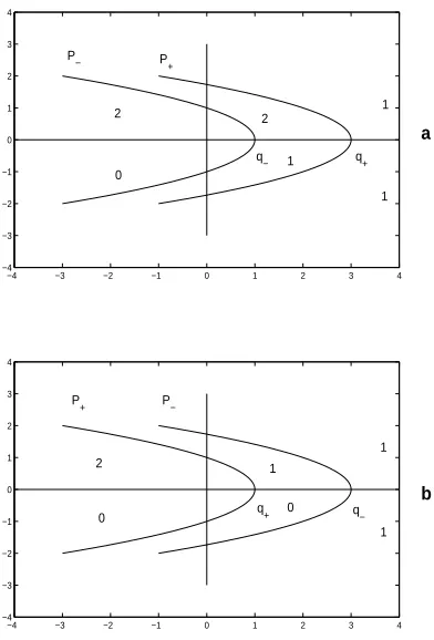
−4 −3 −2 −1 0 1 2 3 4 −4
−3 −2 −1 0 1 2 3 4
−4 −3 −2 −1 0 1 2 3 4
−4 −3 −2 −1 0 1 2 3 4
q
− q+
P− P +
2 2 1
0
1
1
a
b
P
+ P−
q
+ q−
2 1
1
0 0
1
Figure 1. The parabolas given by (32) and (33) for q+ > q− in (a) and for q− > q+ in (b). The dimensions of the subspacesE+
s(λ) and Eu−(λ) are shown, the upper numbers correspond to the former
and the lower numbers correspond to the latter.
Now applying Theorem 3 and Corollary 2 we have the following results concerning the spectrum of
L.
• Both parabolas belong to the essential spectrum ofL.
• The domain lying on the left hand side of both parabolas consists of regular values ofL.
• The domain lying on the right hand side of both parabolas contains all the isolated eigenvalues of
Lthe remaining points of this domain (which are not isolated eigenvalues) are regular values ofL.
• Ifq+> q−, then the domain between the two parabolas is filled with eigenvalues.
• If q+ < q−, then the domain between the two parabolas is filled with points belonging to the
essential spectrum, but they are not eigenvalues.
In this special case ofm= 1 the location of the isolated eigenvalues with respect to the imaginary axis can also be determined. It can be shown that zero is a simple eigenvalue and all other isolated eigenvalues ofLare negative (real) if and only ifU is strictly monotone andf′(U−)<0,f′(U+)<0.
5.2
Flame propagation in a three variable model
Let us consider the travelling wave solutions of the problem
∂τa = L−1A ∂
2
xa−af1(b)
∂τw = L−1W∂2xw−βwf2(b)
∂τb = ∂x2b+af1(b)−αwf2(b)
whereLA, LW, α, β are positive constants (LA, LW are the Lewis numbers) and
with some positiveεandµ. A travelling wave solution, propagating with velocityc, will also be denoted by (a, w, b), and satisfies the boundary conditions
a(y)→1, w(y)→1, b(y)→0 as y→ −∞, (34)
a′(y)→0, w′(y)→0, b′(y)→0 as y→+∞. (35)
Here a is the concentration of the fuel, w is the concentration of an inhibitor species and b is scaled temperature. The travelling wave solution describes a flame propagating with velocityc. The number and stability of travelling waves of this system was investigated in [19]. We proved that the solutions
a, w and b have limits at +∞, that are denoted by a+, w+ and b+. If b+ = 0, then we refer to the travelling wave solution as a pulse solution. Ifb+ >0 then we call it a front solution. In the latter case
a+ = 0 = w+. It was also shown that a saddle-node bifurcation may occur and there can be 1, 2 or 3 travelling wave solutions. The stability of these solutions can also change through Hopf bifurcation. The saddle-node and Hopf bifurcation curves were determined numerically. Here we only show how the method described in the previous Section works for this system to determine the essential spectrum of the corresponding linearizdimen ed operator. The results obtained by the Evans function method will be only cited from [19].
The operator corresponding to a travelling wave solution (a, w, b) of the above system takes the form
LV =
We considerLas an operator defined for theC2 functions in the space
C0={V :R→C3| V is continuous, lim
t→±∞V(t) = 0} endowed with the supremum norm.
NowA±λ are the following 6-by-6 matrices
A±λ =
sinceQ± are lower triangular matrices. Therefore the set of those λvalues for whichn+
c(λ)≥1, that is
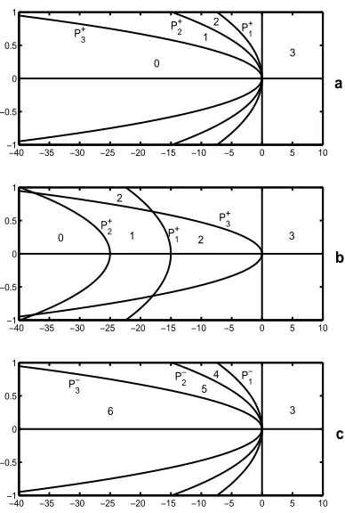
µ= iω (for someω ∈R) is a solution of equation (37), consists of three parabolas, denoted byP1+,P2+,
P3+, see Figure 2 (a) and (b). In Figure 2 (a) the parabolas are shown in the case of a pulse solution, in Figure 2 (b) the parabolas corresponding to a front solution are shown. We define the parabolasP1−,
−40 −35 −30 −25 −20 −15 −10 −5 0 5 10
Figure 2. The parabolas determining the essential spectrum of the operator (36). The dimension of the subspaceE+
s(λ) is shown in part (a) and (b). The dimension of the subspaceEu−(λ) is shown in part
(c). (a) corresponds to pulses, (b) corresponds to fronts.
It can easily be seen that ifλis to the left ofP1+, then both solutions forµof equationL−1A µ2−cµ+
Q±11−λ= 0 have positive real part, and ifλis to the right ofP1+, then one of the solutions has positive real part, the other one has negative real part. The same is true for the other parabolas. Therefore we can determine, for anyλ, the value of n+
s(λ), i.e. the dimension ofEs+(λ), and the value ofn−u(λ), i.e.
the dimension ofE−
u(λ). The values of these numbers are shown in Figure 2 in the different domains
determined by the parabolas. Now applying Theorem 3 and Corollary 2 we have the following results concerning the spectrum ofL.
Proposition 4 1. All parabolas belong to the essential spectrum ofL.
2. The domain lying to the left of all parabolas consists of regular values.
3. The Evans function can be defined in the domain lying to the right of all parabolas.
4. In the case of fronts there are open domains filled with eigenvalues. In the case of pulses this kind of domain does not exist.
ProofWe will use the dimensions of the spacesE+
s(λ),Eu−(λ) as they are given in Figure 2.
1. This statement is a direct consequence of Theorem 3.
2. Ifλis in the domain lying to the left of all parabolas, then dim(E+
s(λ)) = 0, dim(Eu−(λ) = 6, hence
conditions of statement 3 of Corollary 2 are fulfilled, thusλis a regular value.
3. If λis in the domain lying to the right of all parabolas, then dim(E+
s(λ)) = 3, dim(Eu−(λ)) = 3,
hence λ∈Ω, which is the domain of the Evans function.
4. In the case of fronts in the domain lying betweenP1+ andP3+ we have dim(E+
s(λ)) = 2 (see Figure
2b), dim(E−
u(λ)) = 6, hence conditions of Corollary 2 1. are fulfilled, thus any point λ of this
from Figure 2a and 2c we can see that dim(E+
s(λ)) + dim(Eu−(λ)) = 6 holds for any λ∈Cexcept
on the parabolas. Hence according to statements 3. and 4. of Corollary 2 anyλ which is not on the parabolas is a regular value or an isolated eigenvalue.
We can decide whether there are eigenvalues with positive real part by computing the image of a half circle centred at the origin and lying in the right half plane under the Evans functionD. If the image winds around the origin, then by the argument principle there is (at least one) zero ofDin the half circle. Choosing a sufficiently large half circle all the eigenvalues with positive real part are inside the half circle, because an estimate can be derived for the eigenvalues with positive real part. In [19] we computed the Evans function numerically and showed that Hopf bifurcation occurs for some value ofLAbetween 3 and
4. (The bifurcation value was determined more exactly.) ForLA = 3 the image of the half circle does
not wind around the origin, hence there is no zero ofDin the half circle. This value is below the Hopf bifurcation value. ForLA= 4 the image of the half circle winds twice around the origin, hence there are
two zeros ofD in the half circle. This value is above the Hopf bifurcation value. This shows that the Hopf bifurcation value ofLA is between 3 and 4.
5.3
The generalized KdV equation
Let us consider the travelling wave solutions of the problem
∂τu+∂xf(u) +∂x3u= 0 (38)
where f is a twice differentiable convex function with f(0) = 0 = f′(0) and f(u)/u increasing. The motivating example is f(u) = up+1/(p+ 1). This equation has a solitary (travelling) wave solution
u(τ, x) =U(x−cτ) for anyc >0, satisfying the boundary conditionsU(z)→0 as|z| → ∞, see e.g. [17]. (This solution can be given explicitly iff(u) =up+1/(p+ 1)).
The operator determining the stability of a travelling wave solutionU takes the form
LV =V′′′−cV′+ (f′(U)V)′ (39)
The first order system corresponding to the third order equation LV −λV =W can be written in the form (5), wherex= (V, V′, V′′)T,y= (0,0, W)T and
Aλ(t) =
0 1 0
0 0 1
λ−g˙(t) c−g(t) 0
Here we used the notationg(t) =f′(U(t)). NowA±λ are the same matrices
A±λ =
0 1 0 0 0 1
λ c 0
The eigenvalues ofA±λ are determined by the characteristic polynomial
µ3−µc−λ= 0.
Substituting µ = iω into the characteristic equation we obtain Reλ = 0, therefore the set of those λ
values for whichn±
c(λ)≥1 is the imaginary axis.
Since A+λ = A−λ, we have E+
s(λ) = Es−(λ) and Eu+(λ) = Eu−(λ). Hence in the case n±c(λ) = 0 we
have dim(E+
s(λ)) + dim(Eu−(λ)) = 3. In fact, as an elementary computation shows, for Reλ > 0 we
have dim(E+
s(λ)) = 2, dim(Eu−(λ)) = 1. For Reλ <0 we have dim(Es+(λ)) = 1, dim(E−u(λ)) = 2. Now
applying Corollary 2 and Corollary 3 we have the following results concerning the spectrum ofL.
Proposition 5 1. The essential spectrum ofL is the imaginary axis.
2. Ifλis not purely imaginary, then it is either a regular value or an isolated eigenvalue.
In [17] a method is developped for the investigation of the behaviour of the Evans function on the positive half of the real line. The essence of the method is to compute the derivatives of the Evans function at zero and its limit at infinity. It is shown in [17] thatD(λ)→1 as λ→+∞(andλis real). It is also shown thatD(0) = 0 = D′(0) and that D′′(0) <0 if p > 4 and f(u) = up+/(p+ 1). Hence D(λ)<0 for small values ofλ, therefore Dhas a positive real root, that is the solitary wave solution is unstable whenp >4.
References
[1] Alexander, J., Gardner, R., Jones, C., A topological invariant arising in the stability analysis of travelling waves,J. Reine Angew. Math.,410, 167-212, 1990.
[2] Balmforth, N.J., Craster, R.V., Malham, S.J.A., Unsteady fronts in an autocatalytic system,R. Soc.
Lond. Proc. Ser. A,455, 1401-1433, 1999.
[3] Brin, L.Q., Numerical testing of the stability of viscous shock waves,Math. Comp., 70, 1071-1088, 2001.
[4] Chicone, C., Latushkin, Y., Evolution semigroups in dynamical systems and differential equations, Mathematical Surveys and Monographs, 70., American Mathematical Society, Providence, RI, 1999.
[5] Coppel, W.A., Dichotomies in stability theory, Lect. Notes Math. 629, Springer, 1978.
[6] Dalecki˘ı, Ju. L., Kre˘ın, M. G.,Stability of solutions of differential equations in Banach space, Transl. Math. Monographs, Vol. 43. American Mathematical Society, Providence, R.I., 1974.
[7] Doelman, A., Gardner, R.A., Kaper, T.J., Large stable pulse solutions in reaction-diffusion equations,
Indiana Univ. Math. J.,50, 443-507, 2001.
[8] Eastham, M.S.P., The asymptotic solution of linear differential systems, Clarendon Press, Oxford, 1989.
[9] Engel, K.J., Nagel, R.,One-parameter semigroups for linear evolution equations, Springer, 2000.
[10] Evans, J.W., Nerve axon equations IV: The stable and unstable impulse, Indiana univ. Math. J., 24, 1169-1190, 1974/75.
[11] Fiedler, B., Scheel, A., Spatio-temporal dynamics of reaction-diffusion patterns, InTrends in
Non-linear Analysis, Springer-Verlag, to appear.
[12] Gardner, R.A., Zumbrun, K., The gap lemma and geometric criteria for instability of viscous shock profiles,Comm. Pure Appl. Math.,51, 797-855, 1998.
[13] Gubernov, V., Mercer, G.N., Sidhu, H.S., Weber, R.O., On the Evans function calculation of the stability of combustion waves, Austral. Math. Soc. Gaz., 29, 155-163, 2002.
[14] Henry, D.,Geometric theory of semilinear parabolic equations, Springer, 1981.
[15] Lui, R., Stability of travelling wave solutions for a bistable evolutionary ecology model,Nonlinear
Anal.,20, 11-25, 1993.
[16] Palmer, K.J., Exponential dichotomies and Fredholm operators,Proc. Amer. Math. Soc.,104, 149-156, 1988.
[17] Pego, R.L., Weinstein, M.I., Eigenvalues and instabilities of solitary waves, Phil. Trans. R. Soc.
Lond., A 340, 47-94, 1992.
[18] Sandstede, B., Scheel, A., On the structure of spectra of modulated travelling waves,Math. Nachr., 232, 39-93, 2001.
[20] Simon, P.L., Kalliadasis, S., Merkin, J.H., Scott, S.K., On the structure of the spectra for a class of combustion waves, (submitted for publication).