El e c t ro n ic
Jo ur n
a l o
f P
r o b
a b i l i t y
Vol. 11 (2006), Paper no. 50, pages 1342–1371.
Journal URL
http://www.math.washington.edu/~ejpecp/
Eigenvalues of GUE minors
Kurt Johansson
Swedish Royal Institute of Technology (KTH) [email protected]
Eric Nordenstam
Swedish Royal Institute of Technology (KTH) [email protected]
Abstract
Consider an infinite random matrixH = (hij)0<i,j picked from the Gaussian Unitary
Ensem-ble (GUE). Denote its main minors byHi= (hrs)1≤r,s≤i and let thej:th largest eigenvalue
ofHi be µij. We show that the configuration of all these eigenvalues (i, µij) form a
determi-nantal point process onN×R.
Furthermore we show that this process can be obtained as the scaling limit in random tilings of the Aztec diamond close to the boundary. We also discuss the corresponding limit for random lozenge tilings of a hexagon.
Key words: Random matrices; Tiling problems.
1
Introduction
The distribution of eigenvalues induced by some measure on matrices has been the study of random matrix theory for decades. These distributions have been found to be universal in the sense that they turn up in various unrelated problems, some of which do not contain a matrix in any obvious way, or contain a matrix that does not look like a random matrix. In this article, we propose to study the eigenvalues of the minors of a random matrix, and argue that this distribution also is universal in some sense by showing that it is the scaling limit of three apparently unrelated discrete models.
The largest eigenvalues of minors of GUE-matrices have been studied in (Bar01), connecting these to a certain queueing model. It is a special case of the very general class of models analysed in (Joh03). The largeN limit of this model will yield the distribution of all the eigenvalues of a GUE-matrix and its minors.
This process will turn out also to be the scaling limit of a point process related to random tilings of the Aztec diamond, studied in (Joh05a) and of a process related to random lozenge-tilings of a hexagon, studied in (Joh05b).
1.1 Eigenvalues of the GUE
Consider the following point process on Λ =N×R. There is a point at (n, µ) iff then:th main
minor ofH, i.e. Hn, has an eigenvalue µ. We will call this process the GUE minor process. A
central result in this article is that this process is a determinantal point process with a certain kernelKGUE.
For details of what it means for a point process to be determinantal, see section 2. An explicit expression for this kernel is given in the next definition.
Definition 1.2. The GUE minor kernelis
KGUE(r, ξ;s, η) =−φ(r, ξ; s, η) +
−1
X
j=−∞ s
(s+j)!
(r+j)!hr+j(ξ)hs+j(η)e−
(ξ2+η2)/2
,
where φ(r, ξ;s, η) = 0 when r≤s and
φ(r, ξ;s, η) = (ξ−η)
r−s−1√2r−s
(r−s−1)! e
1 2(η
2
−ξ2)
H(ξ−η)
for r > s.
Here,hk(x) = 2−k/2(k!)−1/2π−1/4Hk(x) are the Hermite polynomials normalised so that
Z
hi(x)hj(x)e−x 2
dx=δij,
hk≡0 whenk <0 andH is the Heaviside function defined by
H(t) =
(
1 fort≥0
0 fort <0. (1.1)
Theorem 1.3. The GUE minor process is determinantal with kernel KGUE.
1.4 Aztec Diamond
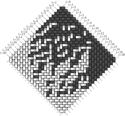
The Aztec diamond of sizeN is the largest region of the plane that is the union of squares with corners in lattice points and is contained in the region|x|+|y| ≤N + 1, see figure 1.
It can be covered with 2×1 dominoes in 2N(N+1)/2 ways, (EKLP92a; EKLP92b). Probability
distributions on the set of all these possible tilings have been studied in several references, for example (Joh05a; Pro03). Typical samples are characterized by having so called frozen regions in the north, south, east and west, regions where the tiles are layed out like brickwork. In the middle there is a disordered region, the so called tempered region. It is for example known that for largeN, the shape of the tempered region tends to a circle, see (JPS98) for precise statement. The key to analyzing this model is to colour all squares black or white in a checkerboard fashion. Let us chose colour white for the left square on the top row. A horizontal tile is of type N, or north, whenever its left square is white. All other horizontal tiles are of type S, or south. Likewise, a vertical domino is of type W, or west, precisely if its top square is white. Other vertical dominoes are of type E.
In figure 1, tiles of type N and E have been shaded. Notice that along the linei = 1, there is precisely one white tile, and its position is a stochastic variable that we denotex11. Along the line
i= 2 there are precisely two white tiles, at positionsx21andx22respectively, etc. In general, letxik
denote thej-coordinate of the k:th white tile along linei. These white points can be considered a particle configuration, and this particle configuration uniquely determines the tiling. It is shown in (Joh05a) that this process is a determinantal point process on N2 = {1,2, . . . , N}2, and the kernel is computed.
We show that this particle process, properly rescaled, converges weakly to the distribution for eigenvalues of GUE described above. More precisely we have the following theorem that will be proved in section 4.
Theorem 1.5. Letµij be the eigenvalues of a GUE matrix and its minors. For eachN, let {xij}
be the position of the particles, as defined above, in a random tiling of the Aztec Diamond of size
N. Then for each continuous function of compact support φ:N×R→R, with 0≤φ≤1,
E
Y
i,j
(1−φ(i, µij))
= lim
N→∞
E
Y
i,j
(1−φ(i,x
i
j−N/2
p
N/2 ))
.
1.6 Rhombus Tilings
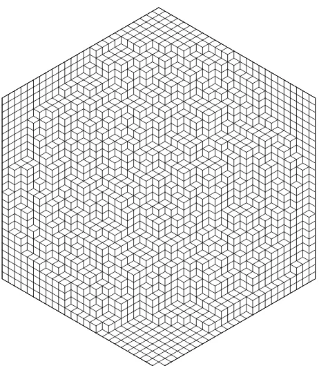
Consider an (a, b, c)-hexagon, i.e. a hexagon with side lengths a,b,c,a,b,c. It can be covered by rhombus-shaped tiles with angles π/3 and 2π/3 and side length 1, so called lozenges. The number of possible such tilings is
a
Y
i=1
b
Y
j=1
c
Y
k=1
i+j+k−1
i+j+k−2.
i=20i=19 i=18i=17
i=16i=15 i=14i=13
i=12i=11 i=10i=9
i=8i=7 i=6i=5
i=4i=3 i=2i=1
j=0 j=1
j=2 j=3
j=4 j=5
j=6 j=7
j=8 j=9
j=10 j=11
j=12 j=13
j=14 j=15
j=16 j=17
j=18 j=19
j=20
Figure 2: Lozenge tiling of a hexagon.
Thus, we can chose a tiling randomly, each possible tiling assigned equal probability. A typical such tiling is shown in figure 2. Just like in the case of the Aztec diamond, there are frozen regions in the corners of the shape and a disordered region in the middle. It has been shown, that when a=b =c =N → ∞, this so called tempered region, tends to a circle, see (CLP98) for precise statement and other similar results.
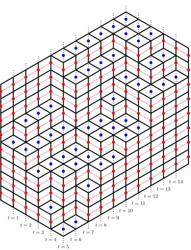
Equivalently, considerasimple, symmetric, random walks, started at positions (0,2j), 1≤j≤a. At each step in discrete time, each walker moves up or down, with equal probability. They are conditioned never to intersect and to end at positions (c+b, c−b+ 2j). Figure 3, the red lines illustrate such a family of walkers, and shows the correspondence between this process and tilings of the hexagon. These red dots in the figure define a point process. (Joh05b) shows that uniform measure on tilings of the hexagon (or equivalently, uniform measure on the possible configurations of simple, symmetric, random walks) induces a measure on this point process that is determinantal, and computes the kernel.
We will show, in theorem 5.4, that the complement of this process, the blue dots in the figure, is also a determinantal process and compute its kernel.
Let us introduce some notation. Observe that along the line t = 1, there is exactly one blue dot. Let its position be x11. Along line t = 2 there are two blue dots, at positions x21 and
x22 respectively, and so on. All these xij are stochastic variables, and they are of course not independent of each other.
We expect that the scaling limit of the process{xij}i,j, as the size of the hexagon tends to infinity,
t= 1 t= 2
t= 3 t= 4
t= 5 t= 6
t= 7 t= 8
t= 9 t= 10
t= 11 t= 12
t= 13 t= 14
0≤φ≤1,
E
Y
i,j
(1−φ(i, µij))
= lim
N→∞
E
Y
i,j
(1−φ(i,x
i
j−N/2
p
N/2 ))
. (1.2)
We will outline a proof of this result by going to the limit in the formula for the correlation kernel, which involves the Hahn polynomials. A complete proof requires some further estimates of these polynomials.
The GUE minor process has also been obtained as a limit at “turning points” in a 3D partition model by Okounkov and Reshetikhin (OR06). We expect that the GUE minor process should be the universal limit in random tilings where the disordered region touches the boundary.
Acknowledgement: We thank A. Okounkov for helpful comments and for sending the
preprint (OR06).
2
Determinantal point processes
Let Λ be a complete separable metric space with some reference measure λ. For example R
with Lebesgue measure or Nwith counting measure. Let M(Λ) be the space of integer-valued and locally finite measures on Λ. A point process x is a probability measure on M(Λ). For example, let x be a point process. A realisation x(ω) is an element of M(Λ). It will assign positive measure to certain points,{xi(ω)}1≤i≤N(ω), sometimes calledparticles, or just points in
the process. In the processes that we will study the number of particles in a compact set will have a uniform upper bound.
Many point processes can be specified by giving their correlation functions, ρn : Λn → R,
n= 1, . . . ,∞. We will not go into the precise definition of these or when a process is uniquely determined by its correlation functions. For that we refer to any or all of the following references: (DVJ88, Ch. 9.1, A2.1), (Joh05c; Sos00).
Suffice it to say that correlation functions have the following useful property. For any bounded measurable functionφ with bounded supportB, satisfying
∞ X
n=1
||φ||n
∞
n!
Z
Bn
ρn(x1, . . . , xn)dnx <∞ (2.1)
the following holds:
E[Y
i
(1 +φ(xi(ω)))] =
∞ X
n=1
1
n!
Z
Λn
φ(x1)· · ·φ(xn)ρn(x1, . . . , xn)dnλ. (2.2)
Correlation functions are thus useful in computing various expectations. For example, if A is some set and χA is the characteristic function of that set, then 1−E[Q(1−χA(xi))] is the
probability of at least one particle in the set A. If the correlation functions of a process exist and are known, this probability can then readily be computed with the above formula.
We will study point processes of a certain type, namely those whose correlation functions exist and are of the form
i.e. then:th correlation function is given as an×ndeterminant whereK : Λ2 →Ris some, not
necessarily smooth, measurable function. Such a process is called adeterminantal point process
and the functionK is called the kernel of the point process.
Let x1, x2, . . . , xN,. . . be a sequence of point processes on Λ. Say that xN assigns positive
measure to the points {xN
i (ω)}1≤i≤NN(ω). Then we say that this sequence of point processes
converges weakly to a point process x, writtenxN →x,N → ∞, if for any continuous function
φof compact support, 0≤φ≤1,
lim
N→∞
E
NN(ω) Y
i=1
(1−φ(xNi (ω)))
=E
N(ω)
Y
i=1
(1−φ(xi(ω)))
. (2.3)
The next proposition gives sufficient conditions for weak convergence of a sequence of determi-nantal processes in terms of the kernels.
Proposition 2.1. Let x1, x2, . . . , xN,. . . be a sequence of determinantal point processes, and
let xN have correlation kernel KN satisfying
1. KN →K,N → ∞ pointwise, for some function K,
2. the KN are uniformly bounded on compact sets in Λ2 and
3. For C compact, there exists some number n=n(C) such that det[KN(xi, xj)]1≤i,j≤m= 0 if m≥n.
Then there exists some determinantal point process x with correlation functions K such that
xN →x weakly.
Proof. We start by showing that there exists such a determinantal point process x. In (Sos00), the following necessary and sufficient conditions for the existence of a random point process with given correlation functions is given.
1. Symmetry.
ρk(xσ(1), . . . , xσ(k)) =ρk(x1, . . . , xk)
2. Positivity. For any finite set of measurable bounded functionsφk: Λk→R,k= 0, . . . , M,
with compact support, such that
φ0+
M
X
k=1
X
i16=···6=ik
φ(xi1, . . . , xik)≥0 (2.4)
for all (x1, . . . , xM)∈IM it holds that
φ0+
N
X
k=1
Z
Ik
The first condition is satisfied for all correlation functions coming from determinantal kernels because permuting the rows and the columns of a matrix with the same permutation leaves the determinant unchanged. For the positivity condition consider the kernelsKN. They are kernels
of determinantal processes so
φ0+
AsN → ∞, this converges to the same expression withK instead ofKN by Lebesgue’s bounded convergence theorem with assumption (2). Positivity of this expression for all N then implies positivity of the limit.
So now we know thatxexists. We need to show thatxN →xTake some test functionφ: Λ→R
with bounded support B. For this function we check the condition in (2.1). The assumption (3) in this theorem implies that the sum is a finite one. Also, ||φ||∞ ≤ 1. Assumption (2) is that the functions KN are uniformly bounded, so in particular they are bounded on B2, so ρk
is bounded onBk. The integral of a bounded function over a bounded set is finite, so this is the
finite sum of finite real numbers, which is finite. Therefore, for eachN, by (2.2),
lim
Condition (3) guarantees that the sum is finite. Lebesgue’s bounded convergence theorem applies because the support ofφis compact and the correlation functions are bounded on compact sets. Thus the limit exists and is
=
3
The GUE Minor Kernel
3.1 Performance Table
Consider the following model. Let{w(i, j)}(i,j)∈Z2
+, be independent geometric random variables
with parameterq2. I.e. there is one i.i.d. variable sitting at each integer lattice point in the first
quadrant of the plane. Let
G(M, N) = max
π
X
(i,j)∈π
where the maximum is over all up/right paths from (1,1) to (M, N). The array [G(M, N)]M,N∈N is called theperformance table.
Each such up/right path must pass through precisely one of (M −1, N) and (M, N −1), so it is true thatG(M, N) = max(G(M −1, N), G(M, N −1)) +w(M, N).
It is known from (Bar01), that (G(N,1), G(N,2), . . . , G(N, M)) for fixedM, properly rescaled, jointly tends to the distribution of (µ1
1, µ21, . . . , µM1 ) asN → ∞ in the sense of weak convergence
of probability measures. We will show that it is possible to define stochastic variables in terms of the values w that jointly converge weakly to the distribution of all the eigenvalues µij of GUE-matrices.
3.2 Notation
We will use the following notation from (Bar01).
1. WM,N is set of M×N integer matrices.
2. WM,N,k is set ofM ×N integer matrices whose entries sum up to k.
3. VM = RM(M−1)/2 where the components of each element x are indexed in the following
way.
x=
x11
..
. . ..
xM1 −1 . . . xMM−−11 xM1 . . . xMM−1 xMM
4. CGC ⊂VM is the subset such thatxij−1 ≥xij−−11 ≥xij.
5. CGC,N are the integer points ofCGC.
6. Let p:CGC →RM be the projection that picks out the last row of the triangular array, i.e. p(x) = (xM1 , . . . , xMM). Likewise, let q :CGC,N → NM, the projection that picks out the last row of an integer triangular array.
3.3 RSK
Recall that a partitionλof kis a vector of integers (λ1, λ2, . . .), where λ1 ≥λ2 ≥. . . such that
P
iλi =k. It follows that only finitely many of the λi:s are non-zero.
A partition can be represented by aYoung diagram, drawn as a configuration of boxes aligned in rows. Thei:th row of boxes isλi boxes long. Asemi-standard Young tableau (SSYT) is a filling
of the boxes of a Young diagram with natural numbers, increasing from left to right in rows and strictly increasing from the top down in columns. The Robinsson-Schensted-Knuth algorithm
(RSK algorithm) is an algorithm that bijectively mapsWM,N to pairs of semi-standard Young
Fix a matrixw∈WM,N. This matrix is mapped by RSK to a pair of SSYT, (P(w), Q(w)). The
P tableau will contain elements ofM:={1,2, . . . , M} only. Construct a triangular array
x=
x1 1
..
. . ..
xM1 −1 . . . xMM−−11 xM1 . . . xMM−1 xMM
where xij is the coordinate of the rightmost box filled with a number at most iin the j-th row of the P(w)-tableau. This is a map from WM,N to CGC,N.
3.4 A Measure on Semistandard Young Tableau
Consider the following probability measure onWM,N. The elements in the matrix are i.i.d.
geo-metric random variables with parameterq2. Recall that a variableXis geometrically distributed with parameter q2, written X ∈ Ge(q2) if P[X = k] = (1−q2)(q2)k, k ≥ 0. The square here will save a lot of root signs later. Such a stochastic variable has expectationa=q2/(1−q2) and
varianceb=q2/(1−q2)2.
Applying the RSK algorithm to this array induces a measure on SSYT:s, and by the corre-spondence above, a measure on CGC,N. Call this measure πqRSK2,M,N. The following is shown in
(Joh00).
Proposition 3.5. Let WM,N contain i.i.d. Ge(q2) random variables in each position. The
probability that the RSK correspondence, when applied to this matrix, will yield Young diagrams of shape λ= (λ1, . . . , λM) is
ρRSKq2,M,N :=
(1−q2)M N
M!
M−1
Y
j=0
1
j!(N −M +j)!×
× Y
1≤i<j≤M
(λi−λj+j−i)2 M
Y
i=1
(λi+ 1)!
(λi+M−i)!
q2k, (3.2)
where k=|λ|=P
iλi.
In other words, the measureπqRSK2,M,M, integrating out all variables not on the last row, isρRSKq2,M,N.
This, together with the following result characterizes the measureπRSK
q2,M,M completely.
3.6 Uniform lift
Proposition 3.2 in (Bar01) states that the probability measureπqRSK2,M,N, conditioned on the last
row of the triangular array beingλ, is uniform on the cone q−1(λ) :={x∈CGC,N:q(x) =λ}. In formulas, this can be formulated as follows.
Proposition 3.7. For any bounded continuous function φ:M×Z→Rof compact support,
E πRSK
q2,M,N[
Y
i,j
(1 +φ(i, xij))] =X
λ
1
L(λ)
X
x∈q−1(λ)
Y
i,j
(1 +φ(i, xij))
where L(λ) is the number of integer points in q−1(λ).
The number of such integer points is given by
L(λ) =Y
i<j
λi−λj+j−i
j−i .
3.8 GUE Eigenvalue measure
It is well know, see for example (Meh91), that the probability measure on the eigenvalues induced by GUE measure on M×M hermitian matrices is
ρGUEM (λ1, . . . , λM) =
1
ZM
Y
1≤i<j≤M
(λi−λj)2
Y
1≤i≤M
exp(−λ2i)
for some constantZM that we need not be concerned with here.
3.9 Uniform lift of GUE measure
(Bar01) shows a result for eigenvalues of minors of GUE matrices that is similar to the above result for partitions. He shows that given the eigenvalues of the whole matrix λ = (λ1 >
· · · > λM), the triangular array of eigenvalues of all the minors are uniformly distributed in
p−1(λ) :={x∈C
GC:p(x) =λ}. Again we can write this more formally.
Proposition 3.10. For any bounded continuous function φ:M×R→R of compact support,
the measure πGUEM satisfies
E[Y
i,j
(1 +φ(i, µij))] =
Z
λ
1 Vol(λ)
Z
p−1(λ)
Y
i,j
(1 +φ(i, µij))
ρGUEM (λ)dMλ.
where Vol(λ) is the volume of the cone p−1(λ).
This volume is given by
Vol(λ) =Y
i<j
λi−λj
j−i .
This situation is then very similar to the measureπRSKq2,M,N above, in the sense that, conditioned
the last row, the rest of the variables is uniformly distributed in a certain cone.
3.11 Scaling limit
We are now in a position to see the connection between the measuresπqRSK2,M,N and πMGUE.
Proposition 3.12. Leta:=E[w(1,1)] =q2/(1−q2)andb:= Var[w(1,1)] =q2/(1−q2)2. Then for any bounded continuous function of compact support φ,
EπGUE
M [ Y
i,j
(1 +φ(i, µij))] = lim
N→∞
EπRSK
q2,M,N[
Y
i,j
(1 +φ(i,x
i j −aN
√
Proof. Plug in the expression for the right hand side in proposition 3.7 and for the left hand side in proposition 3.10. Stirling’s formula and the convergence of a Riemann sum to an integral proves the theorem.
3.13 Polynuclear growth
The measureπRSK
q2,N,M is a version of the Schur process and is a determinantal process onM×N,
by (OR03). We will use the following result from (Joh03).
Proposition 3.14. The process {xij} with the measure described in 3.4 is determinantal with
kernel
KqPNG2,N,M(r, x, s, y) =
1 (2πi)2
Z
dz z
Z
dw w
z z−w
wy+N zx+N
(1−qw)s (1−qz)r
(z−q)N−M
(w−q)N−M. (3.3) For r ≤ s, the paths of integration for z and w are anticlockwise along circles centred at zero with radii such that q <|w|<|z|<1/q. For the case r > s, integrate instead along circles such that q <|z|<|w|<1/q.
This follows immediately from proposition 3.12 and theorem 3.14 in (Joh03).
Having now introduced the PNG-kernel, we can state the following scaling limit result.
Lemma 3.15. Leta=q2/(1−q2) andb=q2/(1−q2)2 as above. The following claims are true
for M fixed.
1. For r, s≤M,
g(r, ξ, N)
g(s, η, N)
√
2bN KN,MPNG(r,⌊aN +ξ√2bN⌋;s,⌊aN+η√2bN⌋)−→KGUE(r, ξ; s, η)
uniformly on compact sets as N → ∞ for a certain function g6= 0.
2. The expression
g(r, ξ, N)
g(s, η, N)
√
2bN KN,MPNG(r,⌊aN +ξ√2bN⌋;s,⌊aN+η√2bN⌋)
is bounded uniformly for1≤r, s≤M and ξ, η in a compact set.
The proof, given in section 6, is an asymptotic analysis of the integral in (3.3). Now everything is set up so we can prove the main result of this section.
Proof of theorem 1.3. According to proposition 3.12,
EπGUE
M [ Y
(1 +φ(i, µij))] = lim
N→∞
EπRSK
q2,M,N[
Y
i,j
(1 +φ(i,x
i j −aN
√
bN ))]. (3.4)
The point processes on the right hand side of this last expression are determinantal. Their kernels can be written
KN(r, ξ, s, η) := g(r, ξ, N)
g(s, η, N)
√
for some functiongthat cancels out in all determinants, and therfore does not affect the corre-lation functions. By lemma 3.15, theseKN satisfy all the assumptions of proposition 2.1. Thus, the point processes that these define converge weakly to a point process with kernelKGUE. This
implies that the measure on the left hand side of equation (3.4), i.e. πMGUEis determinantal with kernelKGUE. The observation that M was arbitrary completes the proof.
4
Aztec Diamond
The point-process connected to the tilings of this shape, described in the introduction was thoroughly analyzed in (Joh05a). The following result is shown.
Proposition 4.1. The process {xij} described in section 1.4 is determinantal on Λ = N×N,
with kernel KNA given by
KNA(2r, x,2s, y) = 1 (2πi)2
Z dz
z
Z dw
w
wy(1−w)s(1 + 1/w)N−s
zx(1−z)r(1 + 1/z)N−r
z
z−w (4.1)
and reference measureµwhich is counting measure onN. The paths of integration are as follows: For r ≤ s, integrate w along a contour enclosing its pole at −1 anticlockwise, and z along a contour enclosing w and the pole at0 but not the pole at1 anticlockwise. For r > s, switch the contours ofz and w.
Based on this integral formula we can prove the following scaling limit analogous to that in lemma 3.15.
Lemma 4.2. The following claims hold.
(1)
g(r, ξ, N)
g(s, η, N)
p
N/2KNA(2r,⌊N/2 +ξpN/2⌋; 2s,⌊N/2 +ηpN/2⌋)−→KGUE(r, ξ;s, η)
uniformly on compact sets as N → ∞ for an appropriate function g6= 0.
(2) The expression
g(r, ξ, N)
g(s, η, N)
p
N/2KNA(2r,⌊N/2 +ξpN/2⌋; 2s,⌊N/2 +ηpN/2⌋)
is uniformly bounded with respect to N for (r, ξ, s, η) contained in any compact set in N×R×N×R.
The proof is based on a saddle point analysis that is presented it section 6. We can now set about proving the main result of this section.
Proof of theorem 1.5. By proposition 4.1, thexi
j form a determinantal process with kernelKNA.
The rescaled process (xij−N/2)/p
N/2 has kernel
KN(r, ξ;s, η) := g(r, ξ, N)
g(s, η, N)
p
N/2KNA(2r, N/2 +ξpN/2; 2s, N/2 +ηpN/2). (4.2)
5
The Hexagon
Consider an (a,b,c)-hexagon, such as the one in figure 3. First we need some coordinate system to describe the position of the dots. Say that the a simple, symmetric, random walks start at
t= 0 and y = 0, 2, . . . , 2a−2. In each unit of time, they move one unit up or down, and are conditioned to end up aty =c−b,c−b+ 2, . . . ,c−b+ 2a−2 at time t=b+cand never to intersect. One realisation of this process is the red dots in figure 3. At timet, the only possible
y-coordinates for the red dots are {αt+ 2k}0≤k≤γt, where
γt=
t+a−1 0≤t≤b b+a−1 b≤t≤c a+b+c−t−1 c≤t≤b+c,
αt=
(
−t 0≤t≤b t−2b b≤t≤b+c.
Let Λa,b,c={(t, αt+ 2k) : 0≤t≤b+c,0≤k≤γt} be the set of all the dots, red and blue.
5.1 A determinantal kernel for the hexagon tiling process
We now need to define the normalised associated Hahn polynomials, ˜qn,N(α,β)(x). These orthogonal polynomials satisfy
N
X
x=0
˜
qn,N(α,β)(x)˜qm,N(α,β)(x) ˜w(Nα,β)(x) =δn,m, (5.1)
where the weight function is
˜
wN(α,β)(x) = 1
x!(x+α)!(N +β−x)!(N−x)!. They can be computed as
˜
qn,N(α,β)(x) = (−N−β)n(−N)n ˜
d(n,Nα,β)n! 3F2(
−n,n−2N−α−β−1,−x
−N−β,−N ; 1),
where
˜
d(n,Nα,β)2= (α+β+N−1−n)N+1
(α+β+ 2N + 1−2n)n!(β+N−n)!(α+N −n)!(N −n)!.
For convenience, let ar=|c−r|andbr =|b−r|. (Joh05b) shows the following.
Proposition 5.2. The red dots form a determinantal point process on the space Λa,b,c with
kernel
˜
Ka,b,cL (r, αr+ 2x; s, αs+ 2y) =−φr,s(αr+ 2x, αs+ 2y)
+
a−1
X
n=0
s
(a+s−1−n)!(a+b+c−r−1−n)! (a+s−1−n)!(a+b+c−s−1−n)!q˜
br,ar
n,γr (x)˜q
bs,as
n,γs (y)ωr(x)˜ωs(y),
where φr,s(x, y) = 0 if r≥sand
φr,s(x, y) =
s−r
y−x+s−r
2
otherwise. Furthermore,
ωr(x) =
((br+x)!(γr+ar−x)!)−1 0≤r ≤b
(x!(γr+ar−x)!)−1 b≤r≤c
(x!(γr−x)!)−1 c≤r ≤b+c
and
˜
ωs(y) =
(y!(γs−y)!)−1 0≤r≤b
((bs+y)!(γs−y)!)−1 b≤r ≤c
((br+y)!(γr+ar−y)!)−1 c≤r≤b+c.
It follows that the blue dots also form a determinantal point process. To compute its kernel we need the following lemma.
Lemma 5.3.
s−r
s−r+2y+αs−2x−αr
2
=
∞ X
n=0
s
(a+s−1−n)!(a+b+c−r−1−n)! (a+r−1−n)!(a+b+c−s−1−n)!q˜
(br,ar)
n,γr (x)˜q
(bs,as)
n,γs (y)ωr(x)˜ωs(y)
when s≥r.
Proof. This proof uses the results obtained in the proof of 5.2 in (Joh05b, equation 3.25). Define convolution product as follows. Forf, g:Z2 →Z, define (f ∗g) :Z2 →Zby
(f ∗g)(x, y) :=X
z∈Z
f(x, z)g(z, y).
Letφ(x, y) :=δx,y+1+δx,y−1. Also let
φ∗0(x, y) :=δx,y
φ∗1(x, y) :=φ(x, y)
φ∗n(x, y) := (φ∗(n−1)∗φ)(x, y).
Set
cj,k :=
1
(a−k)(j−k)!(a−1−j)!
fn,k:=
n k
(n−2a−b−c+ 1)k
(−a−b+ 1)k(−a)k
and finally let
ψ(n, z) :=
n
X
m=0
fn,m a−1
X
j=m
cj,mφ(2j, z)
φ0,1(n, y) :=ψ(n, y)
The dual orthogonality relation to (5.1) is precisely
By equation (3.25), (3.30) and (3.32) of the above mentioned paper,
φ0,r(n, αr+ 2z) =A(a, b, c, r, n)˜qn,γ(br,arr)(z)˜ωr(z),
Inserting this into the orthogonality relation in (5.2) gives
γr
Convolving both sides of the above relation withφ∗(s−r) gives
γr
which, when the left hand side is simplified, gives
γr
Invoking equation (5.1) again to simplify the left hand side and explicitly calculating the right hand side gives
It is easy to check that
A(a, b, c, s, n)
A(a, b, c, r, n) =
s
(a+s−1−n)!(a+b+c−r−1−n)! (a+r−1−n)!(a+b+c−s−1−n)!,
which proves the lemma.
We now need to introduce the normalized Hahn polynomials q(n,Nα,β)(x). These satisfy
Theorem 5.4. The blue dots form a determinantal point process on the space Λa,b,cwith kernel
Proof. It is well known that the complement of a determinantal point processes on a finite set with kernelK is also determinantal with kernel ˜K =I−K, i.e. ˜K(x, y) =δx,y−K(x, y).
Applying this result to our problem, we want to consider δx,yδr,s−K˜a,b,cL (r, x;s, y). We now
separate two cases. Whens≥r see that
K(r, x;s, y) =
is a candidate for the kernel for the blue particles. By lemma 5.3 this simplifies to
K(r, x;s, y) =
We now exploit a useful duality result from (Bor02). It states that
q(n,Nα,β)(x)
Insert this into the formulas above and define the new kernel
This kernel gives the same correlation functions asK, since the extra factors cancel out in the determinants. The new kernel can be written as
Ka,b,cL (r, x;s, y) =
The change of variablesj :=a−1−nputs these expressions on a simpler form, thereby proving the theorem.
uniformly on compact sets inxasN → ∞. For completeness we give the proof of this result in the appendix.
We would like to apply this withp= 12 andγ = 2 to our kernelKLand lettinga=b=c→ ∞,
i.e. we would like to take the limit
K(r, ξ;s, η) =
and formally, if we ignore the fact that this turns into an infinite sum, fors < r we get
K(r, ξ;s, η) =−
Lemma 5.6. Let H be the Heaviside function defined by equation (1.1) above. Then,
(x−y)k−1H(x−y) = (k√−1)!
2k
∞ X
n=−∞ s
n!
(n+k)!hn(y)hn+k(x)e
−y2
. (5.8)
pointwise forx6=y.
The proof is given in section 6.
In view of this result, the infinite series in 5.7 converges and the kernelK is exactly the GUE minor kernel KGUE. The interpretation of this is the following. The distribution of the blue
particles, properly rescaled, tends weakly to the distribution of the eigenvalues of GUE minors as the size of the diamond tends to infinity, equation (1.2). The only thing needed to make this a theorem is appropriate estimates of the Hahn polynomials to control the convergence to the infinite sum.
6
Proof of lemmas
Proof of lemma 5.6. As the Hermite polynomials are orthogonal, there is an expansion of the function in the left hand side of (5.8) of the form
(x−y)k−1H(x−y) =
∞ X
n=−∞
cn(y)Hn(x), (6.1)
where Hn is the n:th Hermite polynomial, as defined in for example (KS98), and where the
coefficients are given by
cn(y) = 1
2nn!√π
Z ∞
−∞
(x−y)k−1H(x−y)Hn(x)e−x 2
dx. (6.2)
It is known that e−x2
Hn(x) =−dxd(e−x 2
Hn−1(x)). Integration by parts and limiting the
inte-gration interval according to the Heaviside function gives
Z ∞
y
(x−y)k−1Hn(x)dx=
Z ∞
y
(k−1)(x−y)k−2Hn−1(x)dx
Repeating this process k−1 times gives
cn(y) =
(k−1)!e−y2
Hn−k(y)
2nn!√π .
Hence,
(x−y)k−1H(x−y) =
∞ X
n=−∞
(k−1)!
2nn!√πHn−k(y)Hn(x)e− y2
=(k√−1)!
2k
∞ X
n=−∞ s
n!
(n+k)!hn(y)hn+k(x)e
−y2
.
Proof of lemma 3.15. Assume first that r ≤ s. By proposition 3.14 we have to consider the
where γr is a circle around the origin with radiusr oriented anticlockwise, q < r1 < r2 <1/q,
and
f(z) = log(z−q)−(1−q2)−1logz. (6.4)
(Here we have ignored the difference between aN +ξ√2bN and its integer part.) Note that
f′(z) = 0 gives z= 1/q. This leads us to choose
and to deformγr2 to a circle Γ oriented clockwise around 1/qwith radius 1/a
p
N/2. The specific choice of radii are convenient for the computations below. Choose
for|t| ≤π/En withC >0.
In the right hand side of (6.5) we make the change of variables
z=z(u) = 1/q−u/apN/2 (6.7)
withu on the unit circle oriented anticlockwise. We obtain the integral
p
for|h|small. Hence, forN sufficiently large,
N(f(z(u))−f(w(0))) =−u2+ 4 +hN(u)/ independent ofN. We also have
apN/2|z(u)−w(t)| ≥1 (6.12)
Hence, for|t| ≤N1/3 we have the bound
It also follows from (6.6), (6.7), (6.9), (6.10), (6.11), (6.14), (6.15) and the dominated conver-gence theorem that the integral in (6.8) converges to
√ infinity. We obtain the integral
√
Expand (v−u)−1 as a geometric series. This turns the expression into
√
and we recognize the classical integral representations of the Hermite polynomials. The expres-sion now becomes
We now turn our attention to the case r > s. Deforming the w-contour through the z-contour in (3.3), we get the same integral as above save for a residue that we pick up atz=w. This is
We see that the argument above goes through for the remaining integral also whenr > s. Using the well known formula
1
the integral in (6.17) becomes
1
It is readily solved as
With our rescaling,x=aN+ξ√2bN andy=aN+η√2bN and the factorsg(r, ξ, N)/g(s, η, N) we see that the integral in (6.17), this is
p whereH is the Heaviside function. AsN → ∞ we get the limit
p
eη2−ξ2
2r−s(ξ−η)r−s−1
(r−s−1)! H(ξ−η), (6.19)
at least forξ 6=η. The caseξ=η is a set of measure zero and is not important. Together with the result for the double integral this completes the proof of claim (1). It remains to show the estimate in claim (2) in this case. But this is easy. The expression in (6.18) is the exact solution of integral (6.17), and since this is bounded inN forξ,ηin a compact set, claim (2) follows.
Proof of lemma 4.2. Assume first thatr ≤s. By proposition 4.1 we have to consider the integral
p
(Here we have ignored the difference betweenN/2 +ξp
N/2 and its integer part.) In the proof of lemma 3.15 we could chose the contours of integration as circles centred at the origin. This cannot be done here.
Note thatf′(z) = 0 gives z= 1. This leads us to choose
r1 = 2−
2
p
N/8
and to deformγr2 to a circle Γ oriented clockwise around 1 with radius 1/
p
N/8. The specific choice of radii are convenient for the computations below. Choose
g(r, ξ, N) =pN−re−ξ2
Parameterize γr1 by
for−π/EN ≤t≤π/EN,EN = 1/
In the right hand side of (6.20) we make the change of variables
z=z(u) = 1−u/pN/8 (6.23)
withu on the unit circle oriented anticlockwise, denotedγ. We obtain the integral
p
for small |h|. Hence, forN sufficiently large
N(f(z(u))−f(w(0))) =−u2+ 4 +hN(u)/
for some constantC >0 depending onr. We also have
foru∈γ,|t| ≤π/EN, by (6.23) and (6.21).
It follows from (6.22), (6.26), (6.27), (6.28) and (6.29) that the part of the integral (6.24) where thet-integration is restricted to N1/3 ≤ |t| ≤π/EN can be bounded by
It also follows from (6.22), (6.23), (6.25), (6.26), (6.28), (6.29), (6.30), (6.31) and the dominated convergence theorem that the integral in (6.24) converges to
p
which is exactly the integral in (6.16). This proves claim (1) in the lemma in the caser ≤s. For r > s we can deform the contours one through the other to get the same integral as we solved above. On the way we pick up the residue of a pole atz=w. It is
One then sees that thei=k term dominates whenN is large.
we see that the integral in (6.32) is
forξ≥η. When ξ6=η this tends to
asN → ∞which together with the corresponding result for the double integral settles claim (1) in the case r > s.
Claim (2) in this case follows from the corresponding result for the double integral,(6.33) and the boundedness of the expression in (6.34).
A
Asymptotics for Hahn polynomials
The Hahn polynomials, as they are defined in (KS98), satisfy
N
The Hermite polynomials are defined as usual:
1
With this notation, the following well known limit theorem holds.
Theorem A.1. Let 0< p <1 andγ ≥0. Let x˜=⌊pN +xp2p(1−p)N(1 +γ−1)⌋ and
uniformly on compact sets.
Now assume that the theorem is true fornandn−1. We wish to show that it is true forn+ 1. There are three term recursion formulas for both Hahn and Hermite polynomials. Let
An=
(n+α+β+ 1)(n+α+ 1)(N −n) (2n+α+β+ 1)(2n+α+β+ 2)
Cn= n(n+α+β+N + 1)(n+β)
(2n+α+β)(2n+α+β+ 1).
Then
AnQn+1(x) = (An+Cn−x)Qn(x)−CnQn−1(x) (A.3)
Hn+1(x) = 2xHn(x)−2nHn−1(x). (A.4)
Solving (A.2) for Qnand inserting into (A.3) gives after some simplification the following:
En+1(x) =
fn+1,N
fn,N
1 + Cn
An −
˜
x An
En(x)−
fn+1,N
fn−1,N
Cn
An
En−1(x). (A.5)
Observe that under our scaling,
An =pN +O(N−1)
Cn =
(1 +γ)n(1−p)
γ +O(N
−1).
Inserting this into equation (A.5) and doing some manipulations gives
En+1(x) =
2x+O(N−1/2)En(x) +
2n+O(N−1/2)En−1(x),
which with our induction assumption is
= 2xHn(x) + 2nHn−1(x) +O(N−1/2)
=Hn+1(x) +O(N−1/2).
This completes the proof.
Applying Stirling’s approximation todα,βn,N,fn,N and the weight function wN(α,β)(x), it is easy to
show that
Corollary A.2. As before, x˜=pN +xp2p(1−p)N(1 +γ−1).
4
p
2p(1−p)N(1 +γ−1)q(α,β)
n,N (˜x)
q
wNα,β(˜x)−→(−1)nhn(x)e−x 2/2
(A.6)
References
[Bar01] Yu. Baryshnikov. GUEs and queues.Probab. Theory Related Fields, 119(2):256–274, 2001. MR1818248
[Bor02] Alexei Borodin. Duality of orthogonal polynomials on a finite set. J. Statist. Phys., 109(5-6):1109–1120, 2002. MR1938288
[CLP98] Henry Cohn, Michael Larsen, and James Propp. The shape of a typical boxed plane partition. New York J. Math., 4:137–165 (electronic), 1998. MR1641839
[DVJ88] D. J. Daley and D. Vere-Jones. An introduction to the theory of point processes. Springer Series in Statistics. Springer-Verlag, New York, 1988. MR0950166
[EKLP92a] Noam Elkies, Greg Kuperberg, Michael Larsen, and James Propp. Alternating-sign matrices and domino tilings. I. J. Algebraic Combin., 1(2):111–132, 1992. MR1226347
[EKLP92b] Noam Elkies, Greg Kuperberg, Michael Larsen, and James Propp. Alternating-sign matrices and domino tilings. II. J. Algebraic Combin., 1(3):219–234, 1992. MR1194076
[Joh00] Kurt Johansson. Shape fluctuations and random matrices. Comm. Math Phys., 209(2):437–476, 2000. MR1737991
[Joh03] Kurt Johansson. Discrete polynuclear growth and determinantal processes. Comm. Math. Phys., 242(1-2):277–329, 2003. MR2018275
[Joh05a] Kurt Johansson. The arctic circle boundary and the Airy process. Ann. Probab., 33(1):1–30, 2005. MR2118857
[Joh05b] Kurt Johansson. Non-intersecting, simple, symmetric random walks and the extended Hahn kernel. Ann. Inst. Fourier (Grenoble), 55(6):2129–2145, 2005. MR2187949
[Joh05c] Kurt Johansson. Random matrices and determinantal processes, 2005. On arxiv.org, math-ph/051003.
[JPS98] William Jockusch, James Propp, and Peter Shor. Random domino tilings and the arctic circle theorem, 1998. arXiv:math.CO/9801068.
[KS98] Roelof Koekoek and Rene F. Swarttouw. The Askey-scheme of
hypergeomet-ric orthogonal polynomials and its q-analogue. Technical Report DUT-TWI-98-17, Delft University of Technology, Delft, The Netherlands, 1998. Available at http://citeseer.nj.nec.com/62227.html.
[Meh91] Medan Lal Mehta. Random Matrices. Academic Press, New York, second edition, 1991. MR1083764
[OR06] Andrei Okounkov and Nikolai Reshetikhin. The birth of a random matrix, 2006. Preprint.
[Pro03] James Propp. Generalized domino-shuffling.Theor. Comput. Sci., 303(2-3):267–301, 2003. MR1990768
[Sag01] Bruce E. Sagan. The symmetric group, volume 203 ofGraduate Texts in Mathemat-ics. Springer-Verlag, New York, second edition, 2001. Representations, combinato-rial algorithms, and symmetric functions. MR1824028
[Sos00] A. Soshnikov. Determinantal random point fields. Uspekhi Mat. Nauk,
55(5(335)):107–160, 2000. MR1799012