El e c t ro n ic
Jo ur
n a l o
f
P r
o
b a b il i t y
Vol. 14 (2009), Paper no. 68, pages 1992–2010.
Journal URL
http://www.math.washington.edu/~ejpecp/
On the Small Deviation Problem
for Some Iterated Processes
Frank Aurzada
∗and Mikhail Lifshits
†Abstract
We derive general results on the small deviation behavior for some classes of iterated processes. This allows us, in particular, to calculate the rate of the small deviations forn-iterated Brownian motions and, more generally, for the iteration ofnfractional Brownian motions. We also give a new and correct proof of some results in[24].
Key words:Small deviations; small ball problem; iterated Brownian motion; iterated fractional Brownian motion; iterated process; local time.
AMS 2000 Subject Classification:Primary 60G18; 60F99; 60G12; 60G52. Submitted to EJP on July 3, 2008, final version accepted August 17, 2009.
∗Technische Universität Berlin, Institut für Mathematik, Sekr. MA 7-5, Straße des 17. Juni 136, 10623 Berlin, Germany,
†St. Petersburg State University, 198504 Stary Peterhof, Dept of Mathematics and Mechanics, Bibliotechnaya pl., 2,
1
Introduction
This article is concerned with the small deviation problem for iterated processes. We consider two independent, real-valued stochastic processesX andY (precise assumptions are given below), define the iterated process by(X◦Y)(t):=X(Y(t)),t∈[0, 1], and investigate the small deviation function
−logP
sup
t∈[0,1]
|X(Y(t))| ≤ǫ
, (1)
whenǫ→0.
The goal of this article is
• to provide general results concerning the order of (1) – given that we know the small deviation probabilities for the processesX andY, respectively, and thatY has acontinuous modification;
• to study some illuminating examples of processes to which this technique can be applied, among them the iteration ofn(fractional) Brownian motions; and
• to show how the technique can be modified if Y has jumps. This is illustrated by several examples, among them theα-time Brownian motion, previously studied in[24]. Here, we give a correct proof of (a weaker version of) the results from[24].
Small deviation problems, also called small ball problems, were studied intensively during recent years, which is due to many connections to other subjects such as the law of the iterated logarithm of Chung type, strong limit laws in statistics, metric entropy properties of linear operators, quanti-zation, and several other approximation quantities for stochastic processes. For a detailed account, we refer to the surveys[18]and[16]and to the literature compilation[19].
The interest in iterated processes, in particular iterated Brownian motion, started with the works of Burdzy (cf. [8] and[9], see also [31]). Iterated processes have interesting connections to higher order PDEs, cf.[1]and[25]for some recent results. Small deviations of iterated processes or the corresponding result for the law of the iterated logarithm are treated in [11](X andY Brownian motions, see also[29]),[12](X Brownian motion,Y =|Y′|withY′being Brownian motion),[24]
(see Section 5 below),[21](X fractional Brownian motion,Y a subordinator), and, most recently,
[22] (X fractional Brownian motion, Y a subordinator, and the sup-norm is taken over a possibly fractal index set).
In Section 2, we give general results under the assumption that the small deviation probabilities of
X and Y, respectively, are known to some extent and that Y has a continuous modification. The proofs for these results are given in Section 3 and the results are illustrated with several examples in Section 4. In Section 5, we treat examples whereY has jumps, in particular, the so-calledα-time Brownian motion, studied earlier in[24].
2
General results
Before we formulate our main results, let us define some notation. We write f g or g f
Moreover, f ® g or g ¦ f say that lim supf/g ≤1. Finally, the strong equivalence f ∼ g means that limf/g=1.
We say that a process X is H-self-similar if(X(c t))= (d cHX(t))for all c >0, where =d means that the finite-dimensional distributions coincide. Recall that, for example, fractional Brownian motion with Hurst parameterHisH-self-similar. However, there are many interesting self-similar processes outside the Gaussian framework, e.g. a strictlyα-stable Lévy process is 1/α-self-similar ([28],[10],
[27]).
Let us consider stochastic processes (X(t))t≥0 and (Y(t))t≥0 that are independent and such that X(0) = 0 and Y(0) = 0 almost surely. We extend X for t < 0 in the usual manner using an independent copy: namely, letX′be an independent copy ofX, and setX(t):=X′(−t)for allt<0. We call this processtwo-sided.
Recall that if X is a classical fractional Brownian motion, it has dependent “wings”(X(t))t≥0 and (X(t))t≤0; hence it does not fit in the scope of the present section. Nevertheless we will show
below how the technique can be adjusted by using the stationarity of increments instead of the independence.
In this section, we assume that
• X is anH-self-similar, two-sided process and
• Y has a continuous modification.
If we know the weak asymptotic order of the small deviation probability of the processesX andY, respectively, we can determine that of the processX◦Y.
Theorem 1. Letθ,τ >0. Then, under the above assumptions, the relations
−logP
sup
t∈[0,1]
|X(t)| ≤ǫ
≈ ǫ−θ
−logP
sup
t∈[0,1]
|Y(t)| ≤ǫ
≈ ǫ−τ (2)
imply
−logP
sup
t∈[0,1]
|X(Y(t))| ≤ǫ
≈ǫ−1/(1/θ+H/τ).
The implication also holds if≈is replaced byor, respectively. For translating lower bounds (i.e.
in the relations above), the assumption that Y is continuous can be dropped.
Remark 2. Note that the resulting exponent is always less thanθ. Therefore, the small deviation probability ofX◦Y is always larger than the one ofX.
Remark 3. In fact, for the proof it is sufficient to know that
−logP
sup
t∈[0,T]
|X(t)| ≤ǫ
≈TθHǫ−θ, whenǫ→0,
Furthermore, provided we know thestrongorder of the small deviation functions, we can prove a result for the strong asymptotic order for that of the iterated process.
Theorem 4. Letτ >0andθ:=1/H>0. Then, under the above assumptions, the relations
−logP
sup
t∈[0,1]
|X(t)| ≤ǫ
∼ kǫ−θ
−logP
sup
s,t∈[0,1]
|Y(s)−Y(t)| ≤ǫ
∼ κǫ−τ (3)
imply
−logP
sup
t∈[0,1]
|X(Y(t))| ≤ǫ
∼κ1/(1+τ)τ−τ/(1+τ)(1+τ)kτ/(1+τ)ǫ−θ τ/(1+τ).
The implication also holds if∼is replaced by®or¦, respectively. For translating lower bounds (i.e.® in the relations above), the assumption that Y is continuous can be dropped.
It is easy to check that this theorem recovers the results from[11], where X andY are Brownian motions, and[12], whereX is a Brownian motion andY =|Y′|withY′being a Brownian motion.
Remark 5. As in Remark 3, it is sufficient to know that
−logP
sup
t∈[0,T]
|X(t)| ≤ǫ
∼kTθHǫ−θ, whenǫ→0,
for allT>0, instead of the self-similarity property and the given small deviations ofX.
Remark 6. A careful reader would wonder why the self-similarity index ofX and the small deviation index ofX should be related byθ :=1/H. In fact, this relation is rather typical for the supremum norm. We refer to[17]for the explanation of this fact in the context of small deviations of general norms. Also see[27; 3].
One may argue that, typically, not the probability in (3) is given but rather the small deviation proba-bility. The following lemma translates from the small deviation probability into (3) (and backwards) if we know that a process satisfies theAnderson property.
Recall that the Anderson property for a random vector Y taking values in a linear space E means that
P(Y ∈A)≥P(Y∈A+e) (4)
for anye∈Eand any measurable symmetric convex setA⊆E, cf.[2]. It is known that any centered Gaussian vector has this property. Another example is given by symmetric α-stable vectors since their distributions can be represented as mixtures of Gaussian ones.
Lemma 7. Let(Y(t))t∈T be a stochastic process with Y(t0) =0a.s. for some t0 ∈ T . Furthermore, assume that Y satisfies the Anderson property. Letτ >0andℓbe a slowly varying function. Then we have
−logP
sup
s,t∈T
|Y(s)−Y(t)| ≤ǫ
if and only if
−logP
sup
t∈T
|Y(s)| ≤ǫ
∼κ2−τǫ−τℓ(ǫ).
Note that the applicability of Lemma 7 depends on the use of the Anderson property. We now state that if X satisfies the Anderson property so does X ◦Y. This makes it possible to use Theorem 4 iteratively.
Lemma 8. Let T be some non-empty index set and let(X(u))u∈Rand(Y(t))t∈T be independent
stochas-tic processes, where X satisfies the Anderson property. Then the process(X(Y(t)))t∈T satisfies the An-derson property.
This shows that, in particular, iterated Brownian motion, the iteration of two (or more general
n) fractional Brownian motions, α-time Brownian motion (defined below), and many other non-Gaussian processes satisfy the Anderson property.
3
Proofs of the general results
Before we prove Theorem 1, we recall a result that translates the small deviation probability into a corresponding result for the Laplace transform.
Lemma 9. Let Y(0) =0almost surely, p>0, andτ >0. Then
−logP
sup
t∈[0,1]
|Y(t)| ≤ǫ
≈ǫ−τ, ǫ→0,
implies
−logEexp
−λ sup
s,t∈[0,1]
|Y(t)−Y(s)|p
≈λ1/(1+p/τ), λ→ ∞.
The relation also holds if≈is replaced by(in the assertion) or(in the assertion), respectively.
Proof:This follows simply from the fact that
1
2 s,tsup∈[0,1]
|Y(t)−Y(s)| ≤ sup
t∈[0,1]
|Y(t)|= sup
t∈[0,1]
|Y(t)−Y(0)| ≤ sup
s,t∈[0,1]
|Y(t)−Y(s)|.
and the de Bruijn Tauberian Theorem (Theorem 4.12.9 in[5]).
Now we can prove Theorem 1.
Proof of Theorem 1: By assumption, for some constantsC1,C1′,C2,C2′ >0 andallǫ >0,
C1′e−C1ǫ−θ ≤P
sup
t∈[0,1]
|X(t)| ≤ǫ
Let
N:= inf
t∈[0,1]Y(t) and M:=t∈sup[0,1]Y(t).
Note that, sinceY is continuous,
Y([0, 1]) = [N,M].
Therefore, by independence ofX andY and by independence of X for positive and negative argu-ments, we have
Now we use theH-self-similarity ofX to see that the last expression equals
E
Analogously one can argue for the second term in (7), which yields that the whole expression in (7) is less than proves the upper bound in the assertion. The lower bound is established in exactly the same way using the lower bound in (5). Note that this argument fails whenY is not continuous, because we
only haveY([0, 1])([N,M].
Now let us prove the strong asymptotics result.
Proof of Theorem 4: Letδ >0. By assumption, for all 0< ǫ < ǫ0=ǫ0(δ),
By repeating the previous proof with (5) replaced by (8), we arrive at
By using the assumptionHθ =1, we clearly have
C22Ee−k(1−δ)ǫ−θ((−N)Hθ+MHθ)=C22Ee−k(1−δ)ǫ−θ(M−N)=C22Ee−k(1−δ)ǫ−θsups,t∈[0,1]|Y(t)−Y(s)|.
Next, by the de Bruijn Tauberian Theorem (Theorem 4.12.9 in[5]), the strong asymptotic logarith-mic order of this Laplace transform, whenǫ→0, is
κ1/(1+τ)τ−1/(1+1/τ)(1+τ)(k(1−δ))1/(1+1/τ)ǫ−θ /(1+1/τ).
Letting δ → 0 proves the upper bound in the assertion. The lower bound follows in exactly the same way using the lower bound in (8). As in the previous theorem, the proof fails when Y is not continuous, because we only haveY([0, 1])([N,M].
Proof of Lemma 7: Clearly,
sup
which implies the inequality in one direction.
≤ X
where we used the Anderson property in the fourth step.
Taking logarithms, multiplying with−(2ǫ)τℓ(2ǫ)−1, taking limits, and using thatℓis a slowly vary-ing function implies that
lim
which finishes the proof.
Proof of Lemma 8: It is sufficient to check (4) for cylinder sets. Fixd≥1 and letBbe a symmetric convex set inRd. Lett1, . . . ,td∈T and fix any functione:T→R1. Define a cylinder
A:=
a:T →R: (a(t1), . . . ,a(td))∈B
and the corresponding random cylinders
AY,e:=
4.1
Iterated Brownian motions
As a first example let us considern-iterated Brownian motions:
where theXi are independent (two-sided) Brownian motions. This process is 2−n-self-similar. The small deviation problem can be solved by using(n−1)-times Theorem 4 and Lemmas 7 and 8.
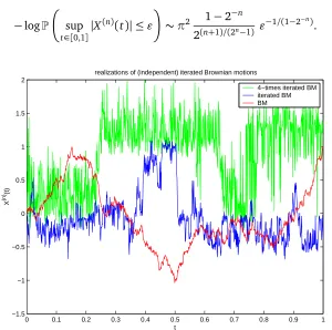
We summarize the result in the following corollary. A simulation forX(1),X(2), andX(4)can be seen in Figure 4.1.
Corollary 10. Let X(n)be the process given by (10), where the Xiare independent two-sided Brownian
motions. Then
−logP
sup
t∈[0,1]
|X(n)(t)| ≤ǫ
∼π2 1−2 −n
2(n+1)/(2n−1) ǫ
−1/(1−2−n)
.
0 0.1 0.2 0.3 0.4 0.5 0.6 0.7 0.8 0.9 1
−1.5 −1 −0.5 0 0.5 1 1.5 2
t
X
(n)
(t)
realizations of (independent) iterated Brownian motions
4−times iterated BM iterated BM BM
Figure 4.1: typical sample paths of iterated Brownian motions
4.2
Iterated two-sided fractional Brownian motions
More generally, one can considern-iterated fractional Brownian motions, given by (10), where this time X1, . . . ,Xn are independent (two-sided) fractional Brownian motions with Hurst parameters
H1, . . . ,Hn, respectively. The processX(n)isH1·. . .·Hn-self-similar. Its small deviation order is given
by
−logP
sup
t∈[0,1]
|X(n)(t)| ≤ǫ
∼cnǫ−τn, where 1
τn =
n
X
j=1
Hj·. . .·Hn (11)
andcnis defined iteratively by
cn:= (1+τn−1)
c1/τn−1
n−1
2c(Hn)
τn−1
τn−1/(1+τn−1)
, c1=c(H1),
Even forn=2, i.e. fractional Brownian motionsX1 andX2 with Hurst parameters H1, H2, respec-tively, this leads to the new result that the small deviation order is
−logP
4.3
The ‘true’ iterated fractional Brownian motion
Note that in the last subsection we obtained the small deviation order for ‘iterated fractional Brow-nian motion’ X◦Y, where X was a two-sidedfractional Brownian motion, i.e. a process consisting of two independent branches for positive and negative arguments, and Y was another fractional Brownian motion (independent of the two branches ofX). We shall now calculate the small devia-tion order for the ‘true’ iterated fracdevia-tional Brownian modevia-tion, namely, usingY as above butX being a centered Gaussian process onRwith covariance
EX(t)X(s) =1 2
|s|2H+|t|2H− |t−s|2H, t,s∈R. (12)
The general result is as follows.
Theorem 11. Let X be a fractional Brownian motion with Hurst index H as given in (12) and Y be a continuous process independent of X satisfying
−logP
where c(H)is the small deviation constant of a fractional Brownian motion.
This theorem can be applied to many processes Y. We recall that (13) can be obtained e.g. via Lemma 7 from the small deviation order. In particular, ifY is also a fractional Brownian motion we get the following result for the ‘true’ iterated Brownian motion.
Corollary 12. Let X be a fractional Brownian motion with Hurst index H2 as given in (12) and Y be a (continuous modification of a) fractional Brownian motion with Hurst index H1(independent of X ). Then
Recall that we obtain the same logarithmic small deviation order as for a two-sided fBM. Moreover, the iteration of n‘true’ fractional Brownian motions provides the same asymptotics as obtained in (11) for the two-sided fBM.
Lemma 13. For anyδ∈(0, 1)there exists Kδ>0such that for all N≤0≤M , for allǫ >0, and for any centered Gaussian process X(t),t∈R, with stationary increments it is true that
P
Proof: To see the upper bound observe that the stationarity of increments and weak correlation inequality (Theorem 1.1 in[15]) yield
P
For the lower bound, using the same arguments in inverse order we get
P Then Lemma 13 yields that, for some constantKδ>0,
= E the last term is bounded from below by
Ef(M+|N|)·Eg(M+|N|)
The first term can be handled as in the proof of Theorem 4, the resulting order is
−logE P
On the other hand, one easily proves that
E P
Lettingδ→0 finishes the proof. The upper bound can be proved along the same lines or by using the Hölder inequality instead of the FKG inequality.
5
The example of
α
-time Brownian motion
5.1
Motivation
LetX be a Brownian motion and Y be a symmetricα-stable Lévy process.
main ingredient of the proof. In fact, it is used thatY([0, 1]) = [N,M], with as aboveN:=inftY(t) andM:=suptY(t), which is not true for thisY.
However, trivially Y([0, 1])( [N,M], and thus the proof in [24]does give a lower boundfor the small deviation probability. The purpose of this section is, among other things, to give a correct proof of the upper bound.
More precisely, the caseβ=2 in the following theorem provides a weaker version of Theorem 2.3 in[24].
Theorem 14. Let X be a two-sided strictly β-stable Lévy process (0 < β ≤ 2) and Y be a strictly
α-stable Lévy process (0< α≤2, independent of X ) that is not a subordinator. Then
−logP
sup
t∈[0,1]
|X(Y(t))| ≤ǫ
≈ǫ−βα/(1+α).
This result implies weaker versions of the results in[24]. In particular, the existence of the small deviation constant and its value are not assured. The same concerns the constants in the law of the iterated logarithm. This should be subject to further investigation.
Note furthermore that we prove the result for general strictlyα-stable Lévy processesY, symmetry (assumed in[24]) is not a feature that would be required here. The only property that is used is self-similarity.
For the sake of completeness let us mention that in the case that Y is an α-stable subordinator (0 < α < 1) and, say β = 2, the result becomes wrong. Namely, in that case X ◦Y is in fact a
symmetric(2α)-stable Lévy process itself, so that we then get that
−logP
sup
t∈[0,1]
|X(Y(t))| ≤ǫ
≈ǫ−2α.
Remark 15. The assertion in Theorem 14 is also true if we take anH-fractional Brownian motion orH-Riemann-Liouville process asX. Then of course,β=1/H.
The proof of Theorem 14 is given in several steps. First note that the lower bound follows from our Theorem 1 and Prop. 3, Section VIII, in[4](the result actually dates back to[30],[23], and[7]). The upper bound follows from Proposition 17 below, as explained there.
5.2
Handling the outer Brownian motion
In order to prove Theorem 14, we shall proceed as follows. In a first step, we show that the small deviation problem of processes that are subordinated to Brownian motion (or more generally, to a strictlyβ-stable Lévy process) are closely connected to the (random) entropy numbers of the range of the inner process (i.e. K = Y([0, 1])). This technique was previously used in [21] and [22]
To formulate the first step, let us define the following notation. For givenǫ >0 and a compact set
K⊆R, let
N(K,ǫ):=min
n≥1,∃x1, . . . ,xn∈R:∀x∈K∃i≤n: |x−xi| ≤ǫ .
These quantities are usually called covering numbers of the setKand characterize its metric entropy. We can get rid of the randomness of the outer processX in the following way. We remark that the following result is inspired by Proposition 3.1 in [22], where it was shown for X being fractional Brownian motion.
Proposition 16. Let X be a (two-sided) strictly β-stable Lévy process, 0 < β ≤ 2. Then there is a constant c0>0such that, for all compact sets K⊆Rand for allǫ >0,
Proof: Let c0 be chosen large enough such that supt≥c
0P(|X(t)| ≤2)≤ e
−1. For N = N(K,c 0ǫβ)
find an increasing sequence t1, ...,tN inKsuch that ti+1−ti ≥c0ǫβ for alli=1, ...,N−1. Then by independence of increments and strict stability ofX we have
P
Recall that in order to prove Theorem 14 we want to get an upper bound for
P
the upper bound in Theorem 14 follows immediately from the next result.
Proposition 17. Let Y be a strictlyα-stable Lévy process and set K=Y([0, 1]). Then there exist small c andδdepending on the law of Y such that
P(N(K,ǫ)< δk)≤e−ck, (14)
for allǫ >0and k= ǫ−α/(1+α)£.
Remark 18. Actually, the investigation of the small deviation probabilities for covering numbers such asP(N(Y([0, 1]),ǫ)<k)is an interesting problem in its own right; and we hope to handle it elsewhere extensively. Here, we just notice that the order of the estimate (14) is sharp and that it is a particular case of a more general fact that can be obtained similarly:
−logP(N(Y([0, 1]),ǫ)<k)≈(kǫ)−α,
which is valid for 1≤ k≤ ǫ−1, 1< α <2, and for 1≤ k ≤δǫ−1+αα, 0< α <1. More efforts are
needed to understand the remaining cases, e.g.ǫ−1+αα ≪k≪ǫ−α, 0< α <1.
We remark here that much is known about the Hausdorff dimension of the range of e.g. Lévy pro-cesses, cf. e.g.[13]for a recent survey or[26]. However, in our case, we require an estimate for the covering numbersN(Y([0, 1]),ǫ)on a set of large measure, which is a related question but requires different methods.
5.3
Proof of Proposition 17
We will now prove inequality (14). For this purpose, let us introduce the notation
N[0,t](ǫ):=N(Y([0,t]),ǫ), t≥0.
For a givent ≥0,N[0,t](ǫ)counts how many intervals are needed in order to cover the range of the process when only looking at the path until time t. A similar quantity was studied in[26], but the results do not seem directly applicable.
LetT =ǫ−α. By scaling we have
PN[0,1](ǫ)≤δk
=PN[0,T](T1/αǫ)≤δk
=PN[0,T](1)≤δk
.
By splitting the time interval[0,T]inkequal pieces, we get intervals of lengthL=T/k≥kα, since
T≥k1+α.
Observe that ifN[0,T](1)≤δk, then there are at most⌈δk⌉points where the function t7→N[0,t](ǫ)
increases. Therefore, there are at least ⌊(1−δ)k⌋ of the intervals, where this function does not increase. Thus, there exists a set of integersJ⊆ {0, . . . ,k−1}such that|J| ≥ ⌊(1−δ)k⌋and there is no increase of covering numbers
N[0,(j+1)L](1) =N[0,j L](1), ∀j∈J. (15)
Letδ <1/2. Notice that the number of choices forJ satisfying|J| ≥ ⌊(1−δ)k⌋can be expressed as 2kP Bk≥ ⌊(1−δ)k⌋
whereBk is a sum ofkBernoulli random variables attaining the values 0 and 1 with equal probabilities. By the classical Chernoff bound for the large deviations ofBkwe see
that this number is smaller than:
δ−δ(1−δ)−(1−δ)k=: exp(δ1k),
whereδ1satisfiesδ1→0, asδ→0.
For a while, we fix an index setJ. We enlarge the events from (15) as follows:
Ωj := ¦N[0,(j+1)L](1) =N[0,j L](1)≤k
⊆ ¦Y((j+1)L)∈Y[0,j L] + [−1, 1],N[0,j L](1)≤k©
= ¦Y((j+1)L)−Y(j L)∈Y[0,j L] + [−1, 1]−Y(j L),N[0,j L](1)≤k
©
=: Ω′j.
Let, as usual, Ft denote the filtration generated by the process Y up to time t. We have, by stationarity and independence of increments,
esssup P(Ω′j|Fj L) ≤ sup
A
{P(Y(L)∈A+ [−1, 1]),N(A, 1)≤k}
≤ sup
A′
P(Y(L)∈A′),N(A′, 2)≤k
≤ sup
A′
P(Y(L)∈A′),|A′| ≤2k
≤ sup
A′′
P(Y(1)∈A′′),|A′′| ≤2 =:c1<1.
By a standard conditioning argument, we find
P
\
j∈J
Ωj
≤P
\
j∈J
Ω′j
≤
Y
j∈J
esssup P
Ω′j|Fj L≤c1|J|≤c1(1−δ)k.
By summing up over all setsJ, we have
P(N[0,1](ǫ)< δk) ≤
X
J:|J|≥⌈(1−δ)k⌉
P
\
j∈J
Ωj
≤ |{J:|J| ≥ ⌈(1−δ)k⌉}|c1(1−δ)k
≤ exp(δ1k)c(11−δ)k;
and we are done with (14) ifδis chosen so small that exp(δ1)c11−δ<1.
5.4
Alternative proof via local times
Here, we give an alternative proof for Proposition 17 whenα >1. In this case, the strictlyα-stable processY possesses a continuous local timeL:
Z
B
L(x)dx=
Z 1
0
1lB(Y(t))dt, for all Borel setsB.
We define L∗= supx L(x), the maximum of local time of the α-stable Lévy process considered on the time interval[0, 1]. It was shown by Lacey ([14]) that
logP(L∗>u)∼ −cuα, asu→ ∞,
Note that, ifN(K,ǫ)<kthen
1=
Z 1
0
1lK(Y(t))dt=
Z
K
L(x)dx ≤L∗
Z
K
1 dx ≤L∗·(ǫk).
Therefore, forǫsmall enough,
P(N(K,ǫ)<k)≤P(L∗>(ǫk)−1)≤exp(−c′(ǫk)−α).
In particular, by lettingk= ǫ−α/(1+α)£we get
P(N(K,ǫ)<k)≤exp(−c′′ǫ−α/(1+α)),
as required in (14).
A similar proof also works for other symmetric Lévy processes, cf.[6], where Lacey’s result is gen-eralized.
Acknowledgement. The first-named author was supported by the DFG Research Center MATHEON
“Mathematics for key technologies” in Berlin. The work of the second author was supported by the DFG-RFBR grant 09-01-91331.
References
[1] H. Allouba and W. Zheng. Brownian-time processes: the PDE connection and the half-derivative generator.Ann. Probab.29(2001), no. 4, 1780–1795. MR1880242
[2] T. W. Anderson. The integral of a symmetric unimodal function over a symmetric convex set and some probability inequalities.Proc. Amer. Math. Soc.6(1955), 170–176. MR0069229
[3] F. Aurzada. Small deviations for stable processes via compactness properties of the parameter set.Statist. Probab. Lett.78(2008), no. 6, 577–581. MR2409520
[4] J. Bertoin.Lévy processes. Cambridge Tracts in Mathematics, vol. 121, Cambridge University Press, Cambridge, 1996. MR1406564
[5] N. H. Bingham, C. M. Goldie, and J. L. Teugels.Regular variation. Encyclopedia of Mathematics and its Applications, vol. 27, Cambridge University Press, Cambridge, 1989. MR1015093
[6] R. Blackburn. Large deviations of local times of Lévy processes.J. Theoret. Probab.13 (2000), no. 3, 825–842. MR1785531
[7] A. A. Borovkov and A. A. Mogul′ski˘ı. On probabilities of small deviations for stochastic pro-cesses.Siberian Adv. Math.1(1991), no. 1, 39–63. MR1100316
[9] .Variation of iterated Brownian motion.Dawson, D. A. (ed.), Measure-valued processes, stochastic partial differential equations, and interacting systems. Providence, RI: American Mathematical Society. CRM Proc. Lect. Notes. 5, 35-53 (1994), 1994. MR1278281
[10] P. Embrechts and M. Maejima.Selfsimilar processes. Princeton Series in Applied Mathematics, Princeton University Press, Princeton, NJ, 2002. MR1920153
[11] Y. Hu, D. Pierre-Loti-Viaud, and Z. Shi. Laws of the iterated logarithm for iterated Wiener processes.J. Theor. Probab.8(1995), no. 2, 303–319. MR1325853
[12] D. Khoshnevisan and T. M. Lewis. Chung’s law of the iterated logarithm for iterated Brownian motion.Ann. Inst. H. Poincaré Probab. Statist.32(1996), no. 3, 349–359. MR1387394
[13] D. Khoshnevisan and Y. Xiao. Lévy processes: capacity and Hausdorff dimension.Ann. Probab.
33(2005), no. 3, 841–878. MR2135306
[14] M. Lacey. Large deviations for the maximum local time of stable Lévy processes.Ann. Probab.
18(1990), no. 4, 1669–1675. MR1071817
[15] W. V. Li. A Gaussian correlation inequality and its applications to small ball probabilities. Elec-tron. Comm. Probab.4(1999), 111–118 (electronic). MR1741737
[16] W. V. Li and Q.-M. Shao. Gaussian processes: inequalities, small ball probabilities and applica-tions. Stochastic processes: theory and methods. Handbook of Statist., vol. 19, pp. 533–597. MR1861734
[17] M. Lifshits and T. Simon. Small deviations for fractional stable processes.Ann. Inst. H. Poincaré Probab. Statist.41(2005), no. 4, 725–752. MR2144231
[18] M. A. Lifshits. Asymptotic behavior of small ball probabilities. Probab. Theory and Math. Statist. Proc. VII International Vilnius Conference, 1999, pp. 453–468.
[19] . Bibliography compilation on small deviation probabilities, available from http://www.proba.jussieu.fr/pageperso/smalldev/biblio.html, 2008.
[20] T. M. Liggett. Interacting particle systems, Grundlehren der Mathematischen Wissenschaften, vol. 276, Springer-Verlag, New York, 1985. MR0776231
[21] W. Linde and Z. Shi. Evaluating the small deviation probabilities for subordinated Lévy pro-cesses.Stochastic Process. Appl.113(2004), no. 2, 273–287. MR2087961
[22] W. Linde and P. Zipfel. Small deviation of subordinated processes over compact sets. Probab. Math. Statist.28(2008), no. 2, 281–304.
[23] A. A. Mogul′ski˘ı. Small deviations in the space of trajectories.Teor. Verojatnost. i Primenen.19 (1974), 755–765. MR0370701
[24] E. Nane. Laws of the iterated logarithm forα-time Brownian motion.Electron. J. Probab. 11 (2006), no. 18, 434–459 (electronic). MR2223043
[26] W. E. Pruitt. The Hausdorff dimension of the range of a process with stationary independent increments.J. Math. Mech.19, 1969/1970, 371–378. MR0247673
[27] G. Samorodnitsky. Lower tails of self-similar stable processes.Bernoulli4(1998), no. 1, 127– 142. MR1611887
[28] G. Samorodnitsky and M. S. Taqqu,Stable non-Gaussian random processes, Stochastic Model-ing, Chapman & Hall, New York, 1994. MR1280932
[29] Z. Shi. Lower limits of iterated Wiener processes.Statist. Probab. Lett.23(1995), no. 3, 259– 270. MR1340161
[30] S. J. Taylor. Sample path properties of a transient stable process. J. Math. Mech. 16 (1967), 1229–1246. MR0208684