Cinderella Goes to School
The Effects of Child Fostering on School
Enrollment in South Africa
Frederick J. Zimmerman
a b s t r a c t
Fostering is a common institution throughout developing countries, where up to 25 percent of children are fostered. An analysis of 8,627 Black South African children suggests that foster children are not less likely than others to attend school, and they tend to move from homes that have difficulty enrolling them in school to homes that are more apt to do so. The net impact of fostering on these children is to reduce the risk of not attending school by up to 22 percent. Fostering therefore provides an im-portant means of improving human-capital investment. Evidence that households foster-in children primarily for their domestic labor is limited.
I. Introduction
Throughout much of the developing world extended family members are integral to the economic choices of the household even when these family mem-bers live in distinct households far away. Considerable research has revealed the importance of the extended family for labor-sharing, risk-pooling (for example, Udry 1994; Cain 1981), and information flows (Rosenzweig and Wolpin 1985). One im-portant institution that unites these interactions is that of child fostering, a common phenomenon in many countries of the developing world, particularly in Africa (Ains-worth 1996; Caldwell 1996; Desai 1992; Page 1989; Silk 1987), but also in Papua New Guinea and Oceania (Silk 1987), in the West Indies (Isiugo-Abanihe 1985), among the rural and urban poor of Brazil (Fonseca 1986), and among indigenous
Frederick J. Zimmerman is an assistant professor in the Department of Health Services and Child Health Institute; University of Washington; 6200 NE 74th St Suite, Seattle, WA 98115-8160; Telephone (206) 616-9392; Fax (206) 616-4623; fzimmer@u.washington.edu. Helpful suggestions of two anony-mous referees are gratefully acknowledged. Any remaining errors are those of the author alone. The data used in this article can be obtained from the author beginning February, 2004 through January 2007. The raw data are in the public domain, and are available at http:/ /www.worldbank.org/html/ prdph/lsms
[Submitted March 1999; accepted January 2002]
ISSN 022-166X2003 by the Board of Regents of the University of Wisconsin System
558 The Journal of Human Resources
peoples of South America (Menget 1988). In regions where fostering is an accepted social norm, the rates of fostering can be very high: 16-25 percent of children in west and southern Africa are fostered away from their biological homes at any given time (Page 1989), and Goody’s (1982) classic study of fostering among the Gonja of southern Ghana finds that about 20 percent of children are fostered at any point in time, and that more than 50 percent of adults had been fostered at one time or another during their childhoods. As HIV infection rates continue to rise in Africa and elsewhere, fostering is likely to become an ever-more-common means of caring for children when one or both parents become disabled.
The prevalence of child fostering should make it of interest to population and development economists for two reasons. First, with such a large proportion of chil-dren experiencing fosterage at one point or another during their lives, it is important to understand the effects of this institution on children’s schooling, health, and nutri-tion outcomes. Calculanutri-tions using the data source discussed in this article reveal that school enrollment in South Africa averages 90 percent for Black children overall, but only 88 percent for fostered children. Second, most studies modeling household decisions over fertility, human capital investment, asset accumulation, and labor sup-ply have focused on the household as the unit of analysis—and certainly as the unit of data collection. Yet if the household is able to gain access to additional domestic labor through fostering, or is able to educate children through extended family net-works in the face of binding household-level constraints, or is able to practice ex-post family planning by fostering out children, or if individual members are able to influence intrahousehold bargaining outcomes by fostering children in or out, then clearly the focus on the household needs to be expanded to consider the important effects of the extended family network (Isiugo-Abanihe 1985).
This paper evaluates two of the most commonly hypothesized reasons for foster-ing—demand for domestic labor and human capital investment—as well as the ef-fects of fostering on human capital investment in children. An important contribution of this paper is to highlight the benefits of fostering to the children involved, and thereby to show the institution of fostering as a demographically flexible response to the risks and challenges of resource-poor environments.
This paper’s focus is on Blacks in South Africa. Empirical tests are developed to ascertain the extent to which Black South Africans are responding to the several motivations for fostering children into their households. This paper extends Ains-worth’s (1996) study of fostering in Coˆte d’Ivoire, and reaches somewhat different conclusions. Where Ainsworth finds fostering to be largely a transfer of domestic labor, this analysis finds that for South Africa, evidence for the domestic labor moti-vation is limited, and that other motimoti-vations, such as the desire to build social ties, may be at play as well. This paper also tests the effects of fostering on children’s school enrollment rates. It is shown that children who are fostered to close relatives (90 percent of all foster children) are no less likely to attend school than children who live with their biological parents. They also spend no more time on household chores than children living with their biological parents. Moreover, the homes from which children are typically fostered out are less able to send children to school than the homes to which they are sent, so that the net effect of fostering is to considerably improve the school enrollment rates of the children involved.
Zimmerman 559
institutional introduction to the practice of child fostering. Section III develops a theoretical model of child fostering that captures two of the major hypothesized motivations for fostering-in children: domestic labor and nonmaterial benefits such as cementing social ties. Section IV presents the data with descriptive statistics and describes the econometric approach. Sections V and VI implement the empirical tests. Section V tests the reasons for fostering-in, and Section VI tests the effects of fostering on the human capital investment in children, through an analysis of enrollment rates. Section VII concludes.
II. The Institution of Child Fostering
super-560 The Journal of Human Resources
vised, and fostering accordingly provides one way of increasing the household’s family labor endowment.
The anthropological literature suggests that the institution of fostering is indeed a response to many of these market imperfections and features of the institutional environmental. (See Gage, Sommerfelt and Piani 1997; Ainsworth 1996; Page 1989; Bledsoe and Isiugo-Abanihe 1989; Silk 1987; Isiugo-Abanihe 1985; Goody 1982). Fostering is considered so institutionally useful that Page (1989) suggests that foster-ing is not a departure from a cultural norm, but rather an integral part of the norm. The anthropological literature therefore echoes what economists would expect from an institutional analysis of the incentives for fostering.
Reasons for accepting fostering children into the household include: the demand for domestic labor, insurance motivations emotional bonds and companionship, and social or political prestige. Reasons for fostering children out include: a desire to improve the health, educational or job prospects of the child; a desire to cement social ties; changes in conjugal status; insurance motivations; and social, religious, or political prestige. Probably the most commonly cited reason in the anthropological literature for the existence of fostering as an institution is to strengthen kinship and social ties across households, and indeed the exchange of sons and daughters with other families has long been an effective means of cementing social relations (and not just in developing countries1). Goody (1982) cites the example of a boy who
fostered to cement the friendship between two important chiefs. A second major reason is ‘‘. . . for educational, economic, or political opportunities’’ (Silk 1987; also, Page 1989; Goody 1982), although these may include very informal forms of human capital such as developing the moral character of a difficult child (Silk 1987).
Anthropologists have typically written about fostering as a cultural institution and have devoted less attention to statistical analyses of the effects of fostering on chil-dren.2Despite the attention the institution of fostering has received from
anthropolo-gists, there has been very little published in the economics literature on fostering, and nothing at all on the effects of fostering on children’s well-being. This is a curious omission given economists’ interest in resource allocation, human-capital investment, and especially how these decisions are affected by multiple market im-perfections. If fostering is as common and as normative as the anthropological evi-dence suggests, then, by providing an opportunity to transfer offspring across resi-dence units, fostering might constitute a highly flexible way for households to take advantage of economic opportunities that market imperfections would otherwise close to them. Put differently, child-fostering may be an efficient response to an imperfect world.
Becker’s theory of the family (Becker 1991), taking its cue from evolutionary biology, predicts that, because foster children do not share as many genes with their caretakers as do children living with their biological families, households should allocate fewer scarce family resources to foster children than to biological children.
1. Most famously for the Hapsburgs:Bella gerunt alii, tu, felix Austria, nubes!
Zimmerman 561
There should be, as it were, a ‘‘Cinderella Effect,’’ such that foster children would be likely to work more and would be less likely to attend school than biological children.3Yet, as Yoram Ben Porath (1980) has pointed out, not all exchange need
be immediately reciprocal. It is possible, in other words, that households may treat foster children as well as their biological children in the interest of complying with social norms, cementing social ties or providing insurance for themselves in times of old age or hardship. The return need not be immediate, explicit, or even certain, but might take the form of participation in an entire set of social norms, the sum of which is beneficial to the household. If so, one need not expect the Cinderella effect to be particularly pronounced, or even to exist at all.
Testing the existence and magnitude of the Cinderella effect among black South African foster children is an important contribution of this paper. However, the full effect of fostering on children is not well measured by the Cinderella effect, since even foster children who are treated poorly in foster homes might still be better off relative to their treatment in their own biological families. This would be particularly true if fostering-out of a crisis in the sending family, such as a death of a parent, through which the family becomes unable to adequately care for the children. Thus, in additional to the Cinderella effect, this paper tests the hypotheses that foster chil-dren typically move from low-resource families without good access to educational opportunities to families with more resources and better access to education. Regard-less of the immediate reasons for fostering, parents will presumably do everything possible to place their children in good homes, and this migration effect is presum-ably positive. The net effect of fostering will emerge out of the relative strengths of this migration effect and the Cinderella effect.
III. A Model of Child Fostering and School
Enrollment
Assume a household has utility that depends on six things: its per-capita consumption of market goods (C); its per-capita consumption of home-pro-duced goods and services (Z); the leisure time of its adult women (L); social ties it has with other households (S); and the average level of education of its biological children (Ec) and of any foster children the household might have (Ef). In what
fol-lows, the subscriptcwill represent biological children, and the subscriptfwill repre-sent foster children. The leisure time of adult men is assumed to be exogenous to the decisions modeled here. Finally, the household derives utility indirectly from fostering, for example because fostering-in household enjoy caring for their foster children, or because these children confer benefits on them by helping them negotiate the modern economy or by solidifying their ties to other households. The reasons social ties contribute to utility are twofold. Households in South Africa (and no doubt elsewhere) have been shown to intrinsically value their social connections to other households (May 1996). In addition, these ties form a kind of risk-managing social network upon which the household may call in times of need (May 1996; See also Platteau 1991 1994; Udry 1994; Fafchamps 1992).
562 The Journal of Human Resources
The number of biological children that the households has (Nc) is assumed to be
fixed, as are the numbers of adult women (W0) and adult (M0). However, the
hold may adjust the number of its children by fostering children in or out. The house-hold’s utility function may be written:
(1) u⫽u(C,Z,L,Ec,Ef,S;W0,M0,Nc)
In this formulation, fostering children in or out does not directly contributed to the household’s utility, but doing so creates indirect benefits, such as social ties (S), that do, and may contribute to the probability that the biological children will be enrolled in school. Fostering-in children may also release household adult labor time from home production, thereby raising household income and/or increasing the leisure time of adult women.
The value of the social ties depends on the number of children fostered in or out (Nf), and the education provided to such children (Effor children fostered in E˜ffor
children fostered out to another household).
(2) S⫽θ(Nf,Ef,E˜f)
The household has some technology for producing home-produced goods and ser-vices using market inputs (Xz), and time of adult women (Tzw), biological children
(Tzc), and foster children (Tzf). Note that there is no reason to suppose that biological
children and foster children are equally productive per unit of time; moreover, foster children may require training or supervision differently than biological children. Ac-cordingly, the time of foster children and biological children enters the production function separately:
(3) Z⫽ ζ(Xz,Tzw,Tzc,Tzf) W0⫹M0⫹Nc⫹Nf
with ζ′i ⬎0;ζ″i ⬍0 fori⫽1,2,3,4
Note the adjustment of total household production for household size in Equation 3 to arrive at per-capita consumption of home-produced goods and services. This formulation is clearly a simplification (but without loss of generality), given the extensive evidence both of unequal distribution of resources within the household (for example, Rose 1999; Haddad, Hoddinott, and Alderman 1997; Lundberg and Pollak 1993; Folbre 1984) as well as of economies of scale inherent in certain home-produced services, such as cooking and heating (Lanjouw and Ravallion 1995).
For both foster children and biological children, the household determines the allocation of their time between home-production (Tzf,Tzc) and school (Tef,Tec),
sub-ject to an overall time constraint:
(4) Nf⫽Tzf⫹Tef(foster children)
Nc⫽Tzc⫹Tec(biological children)
whereNfis the (endogenous) number of foster children in the household. A
exoge-Zimmerman 563
nously determined and is not systematically different between foster children and biological children.4
The time endowment of the household’s adult women is divided between their leisure time (L) their time in home production (TZW) and their time in market work
(Tmw):
(5) W0⫽L⫹Tzw⫹Tmw
The household produces education for its children according to a production function that includes the child’s time and purchased inputs for education (Xc,Xf). Households
simultaneously determine the time and money allocations to education, and deter-mine whether it would be optimal to enroll the child in school. The average propen-sity to enroll the foster children and the biological children in school is:
(6) Ei⫽
ξ(Tei,Xi;A,Gi)
Ni
fori⫽{c,f}
whereArepresents household assets andGiis matrix (one vector per child) of
child-specific attributes, such as age and ability, and including whether the child is a foster child. Such characteristics might plausibly be at least partly endogenous, since house-holds have some choice in the children they foster in or out. Included in household assets are the household’s land endowment, the education levels of its adult mem-bers, the average health status of memmem-bers, and the household’s access to water, fuel wood, and health providers.
The model is closed with the household’s budget constraint, which equates the sum of exogenous income (R, which includes men’s earnings) and the women’s wage earnings (wherewis the exogenous market wage) to the sum of household consumption expenditures and investments in education and inputs into household production:
(7) R⫹w⋅Tmw⫽C⋅(W0⫹M0⫹Nc⫹Nf)⫹Xz⫹Xf⫹Xc
The choice variables in the model are the use of children’s time (Tec,Tzc,Tef,Tzf),
the use of the time of the adult women (Tmw,Tzw,L), the household’s expenditures
(C,Xc,Xf,Xz), the children’s educational levels (Ec,Ef), the level of home-produced
goods (Z), and the number of foster children (Nf). The exogenous variables include
the household’s exogenous income (R), the women’s market wage (w), household assets (A), and demographic variables (W0,M0,Nc).
The model may be solved by using the time constraints Equations 4 and 5 to substitute out the children’s and women’s time from the production of home goods, Equation 3; then substituting this function into the Utility Function 1 replacing the home-goods variable; substituting the children’s Education Functions 6 similarly into the utility function; rearranging the Budget Constraint 7 and substituting out the consumption of market goods from the utility function. The utility function can
564 The Journal of Human Resources
then be maximized in the usual way, and the first-order conditions on the remaining choice variables may be combined to determine the optimal levels of the choice variables as a function of exogenous variables.
The household’s choice for the optimal number of foster children may be repre-sented as:
(8) N*f ⫽Nf(W0,M0,Nc,A,R,w)
Similarly, the household chooses the optimal level of education for its biological children and its foster children:
(9) E*i ⫽Ei(W0,M0,Nc,A,R,w) fori⫽{c,f}
IV. Data and Econometric Specification
Data are available for empirical estimation of these equations from the South African Project for Statistics on Living Standards and Development (PSLSD), a nationally representative data set collected by the South African Labour and Development Research Unit (SALDRU) of the University of Cape Town, in 1993, with funding in part from the World Bank.
As is usual in this context, data were collected at the household level, with the household in mind as the unit of analysis. Clearly this sampling approach creates some challenges for the project here, where it would have been preferable to collect data directly on the extended family networks within which fostering typically takes place.
Data were available on household composition and assets, community-level schooling variables (such as whether a primary or secondary school was present), and children’s gender, age and school enrollment status. In addition, data were col-lected on the amount of time each household member spent collecting wood and water. Fostered-in children and households were identified as those situations in which the child did not identify any household member as his or her father or mother. No data were available on the biological families of foster children.
Two distinct samples are used in the analyses that follow. A household-level sam-ple, comprising 3,320 black households with school-age children (that is, aged 7– 17) for which household’s complete data were available was used to estimate the likelihood of fostering-in children and the effects of fostering on household income. A child-level sample of 8,627 children aged 7–17 with complete data was used to predict enrollment. Descriptive statistics for the household sample are presented in (Tables 1 and 2, and for the child-level sample in Table 4.
iden-Zimmerman 565
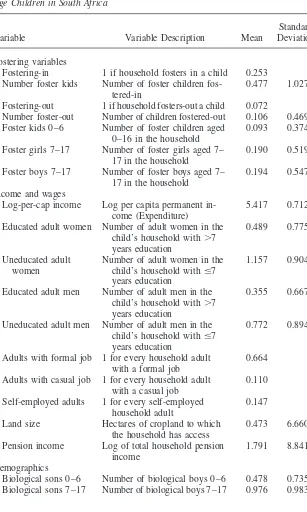
Table 1
Variable Definitions and Descriptive Statistics for Black Households with School-Age Children in South Africa
Standard
Variable Variable Description Mean Deviation
Fostering variables
Fostering-in 1 if household fosters in a child 0.253
Number foster kids Number of foster children fos- 0.477 1.027 tered-in
Fostering-out 1 if household fosters-out a child 0.072
Number foster-out Number of children fostered-out 0.106 0.469 Foster kids 0–6 Number of foster children aged 0.093 0.374
0–16 in the household
Foster girls 7–17 Number of foster girls aged 7– 0.190 0.519 17 in the household
Foster boys 7–17 Number of foster boys aged 7– 0.194 0.547 17 in the household
Income and wages
Log-per-cap income Log per capita permanent in- 5.417 0.712 come (Expenditure)
Educated adult women Number of adult women in the 0.489 0.775 child’s household with⬎7
years education
Uneducated adult Number of adult women in the 1.157 0.904
women child’s household withⱕ7
years education
Educated adult men Number of adult men in the 0.355 0.667 child’s household with⬎7
years education
Uneducated adult men Number of adult men in the 0.772 0.894 child’s household withⱕ7
years education
Adults with formal job 1 for every household adult 0.664 with a formal job
Adults with casual job 1 for every household adult 0.110 with a casual job
Self-employed adults 1 for every self-employed 0.147 household adult
Land size Hectares of cropland to which 0.473 6.660
the household has access
Pension income Log of total household pension 1.791 8.841 income
Demographics
566 The Journal of Human Resources
Table 1(continued)
Standard
Variable Variable Description Mean Deviation
Biological daughters Number of biological girls 0–6 0.452 0.726 0–6
Biological daughters Number of biological girls 7– 0.986 1.001
7–17 17
Adults over 65 Number of adults over 65 0.427 0.655
Time on wood and Person-weeks per week the 0.569 1.006
water household spends collecting
fuelwood and water Human capital
Full enrollment 1 if all children in household 0.946 are enrolled in school
Maximum female edu- Maximum years of female edu- 4.519 3.277
cation cation in household
Maximum male edu- Maximum years of male educa- 3.666 3.608
cation tion in household
Primary school 1 if there is a primary school in 0.778 the community
Secondary school 1 if there is a secondary school 0.548 in the community
Travel time to school Minutes of travel time to school 30.724 28.303 Per-pupil cost of edu- Hundreds of Rand in total 0.426 1.176
cation monthly educational cost per
pupil
Cluster education av- Cluster-average of (years of ed- ⫺1.079 0.651
erage ucation⫹6⫺age)
Distance to doctor Distance to nearest doctor in ki- 11.929 16.781 lometers
Distance to pharmacist Distance to nearest pharmacist 21.908 26.399 in kilometers
Distance to comm Distance to nearest community 11.428 23.700 health worker health worker in kms.
Social attributes of the household
Percent of children with Fraction of children in house- 0.366 0.300
father hold whose father is present
Enough water 1 if the household reports al- 0.794 ways getting enough water
Days sick Days sick of all household 0.578 1.152
member in previous week
Zimmerman 567
tify fostering-out households are not available in these data, only fostering-in deci-sions are estimated here.
The social norm in much of Africa when more than one child is fostered out is to try to keep siblings together where possible (Page 1989); for this reason and because the number of children fostered in or out must be an integer, it is difficult for households to use the institution of fostering to achieve exactly the ideal number of foster children. Accordingly, the fostering-in equation will be estimated in a probit framework using the household-level data, in which the latent propensity to foster is represented by a linear approximation with a normally distributed error term (εi):
(10) N*fi ⫽α0⫹α1W0⫹α2M0⫹α3Nc⫹α4R⫹α5w⫹Aβ1⫹Gcβ2⫹εi,
and a household is observed to foster in children iffN*f ⬎0. As discussed above,
the data are not sufficiently rich to enable estimation of a similar fostering-out equa-tion.
Supply side issues play a role in whether a given household actually fosters chil-dren in—that is, whether other households will be willing to foster-out a child to a particular household. One possibility is that households will be more willing to foster a child to a particular household if they feel that household is likely to send the child to school. A good indicator of this likelihood is whether the household sends all of its own children to school. Since this decision is itself endogenous to the household’s fostering-in decision, a two-stage approach is adopted. In the first stage, a probit regression predicts the probability that a household enrolls all of its own children in school. A binary variable is then created to indicate whether there is a greater than 95 percent predicted probability that the household will enroll all of its children. This cutoff was chosen because 94.6 percent of the households in the sample enroll all of their children. Thus, the predicted variable represents whether the household is more likely than average to enroll all its children. In the second stage, this predicted enrollment indicator is included as an explanatory variable in the fostering-in regres-sion equation.5
Variables excluded from the main, fostering-in regression that were used to predict full enrollment were the job status of the household head and community education characteristics (for example, whether a primary school was nearby and the average educational-attainment level of the community). The identifying assumption of this two-stage approach is that these variables are correlated with enrollment, but uncor-related with the fostering decision, except through enrollment. This assumption seems reasonable for the community-level variables. For the job-status variables, measured at the household level, the assumption is that job status affects the opportu-nities afforded foster children, that is, those in formal-sector jobs and possibly also self-employment can offer better political and economic connections to a foster child than those in casual employment (Page 1989; Goody 1982). A chi-squared test strongly rejects at the 1 percent level the null hypothesis that the coefficients on the excluded variables are jointly zero (χ2
⫽45.9, 7 degrees of freedom).
568
The
Journal
of
Human
Resources
Table 2
Household-Level Regressions of Fostering, Enrollment, and Income among Black South African Households with School-Age Children
Full Log-Per-A.E.
Fostering-In Fostering-In Enrollment Income
(Probit) (Probit) (Probit) (OLS)
Marginal Marginal Marginal Marginal
Effect |t| Effect |t| Effect |t| Effect |t|
Fostering-in ⫺0.075 (2.80)**
Educated adult women ⫺0.028 (2.06)* 0.005 (0.42) 0.004 (1.83) 0.039 (2.44)* Uneducated adult women 0.011 (1.17) 0.009 (0.90) 0.001 (0.10) ⫺0.143 (9.96)**
Educated adult men ⫺0.011 (0.80) 0.013 (0.98) 0.003 (1.05) 0.044 (2.09)*
Uneducated adult men 0.021 (2.30)* 0.010 (1.03) ⫺0.001 (0.20) ⫺0.149 (10.85)**
Adults with formal job ⫺0.002 (0.21) ⫺0.002 (0.36) 0.156 (6.71)**
Adults with casual job 0.005 (0.20) 0.000 (0.11) ⫺0.064 (2.40)*
Self-employed adults 0.007 (0.42) ⫺0.002 (0.22) 0.181 (7.59)**
Adults over 65 0.136 (13.65)** 0.144 (14.58)** 0.001 (0.24) ⫺0.089 (5.40)**
Land size ⫺0.001 (1.04) 0.000 (0.46) 0.002 (1.19) 0.003 (2.63)**
Time on wood and water 0.018 (1.71) 0.011 (0.95) ⫺0.001 (1.32)
Pension income 0.001 (1.37) 0.001 (1.44) 0.000 (0.150) 0.002 (1.52)
Distance to doctor ⫺0.001 (2.06)* ⫺0.001 (2.03)* Distance to pharmacist 0.001 (1.71) 0.001 (1.80) Distance to community health 0.000 (0.78) ⫺0.001 (1.52)
Zimmerman
569
Primary school nearby 0.001 (0.04) ⫺0.002 (0.78)
Secondary school Nearby ⫺0.017 (0.84) 0.004 (1.89)
Per-pupil cost of education 0.001 (0.13) 0.027 (2.07)*
Cluster-average education attained ⫺0.040 (2.85)** 0.007 (5.05)**
Enough water ⫺0.025 (1.11) ⫺0.030 (1.34) ⫺0.003 (0.72) 0.096 (2.97)**
Days sick ⫺0.018 (2.42) ⫺0.017 (2.26)* 0.001 (0.72) 0.021 (2.05)*
Long-term illnes 0.034 (1.28) 0.019 (0.73) ⫺0.006 (1.89) 0.043 (1.14)
All children 0–6 ⫺0.001 (0.65)
All girls 7–17 0.012 (6.42)**
All boys 7–17 0.010 (5.58)**
Percent of children with father 0.005 (1.60)
Biological sons 0–6 0.014 (1.10) ⫺0.001 (0.06) ⫺0.050 (3.48)**
Biological Sons 7–17 ⫺0.152 (10.64)** ⫺0.120 (9.73)** ⫺0.035 (3.27)**
Biological daughters 0–6 ⫺0.015 (1.20) ⫺0.023 (1.91) ⫺0.038 (2.47)*
Biological daughters 7–17 ⫺0.167 (12.11)** ⫺0.126 (11.01)** ⫺0.037 (3.46)**
Predicted income 0.007 (0.19)
Predicted enrollment 0.187 (10.70)**
Observations 3,320 3,320 3,320 3,320
Pseudo R-squared; R-squared 0.24 0.21 0.24 0.38
Chi-squared (df ) 543.25 (27) 525.73 (33) 295.95 (31)
Absolute value oft-statistics in parentheses
570
The
Journal
of
Human
Resources
Table 3
Fostering-In Probit Regressions by Age and Gender of Child among Black South African Households with Scholl-Age Children
Fostering-In Fostering-In Fostering-In Fostering-In Girls Aged 0–6 Girls Aged 7–17 Boys Aged 0–6 Boys Aged 7–17
Marginal Marginal Marginal Marginal
Effect |t| Effect |t| Effect |t| Effect |t|
Educated adult women 0.001 (0.16) ⫺0.010 (1.22) 0.006 (1.61) ⫺0.030 (3.52)**
Uneducated adult women 0.010 (3.30)** 0.002 (0.34) 0.010 (3.65)** 0.001 (0.21)
Educated adult men 0.001 (0.13) ⫺0.009 (1.12) 0.006 (1.45) ⫺0.009 (0.91)
Uneducated adult men 0.004 (1.47) 0.019 (3.10)** 0.001 (0.18) 0.012 (2.26)*
Adult over 65 0.014 (4.22)** 0.061 (9.99)** 0.016 (4.18)** 0.059 (8.98)**
Biological sons 0–6 ⫺0.003 (0.61) 0.009 (1.14) ⫺0.007 (1.59) 0.017 (2.26)*
Biological sons 7–17 ⫺0.015 (3.22)** ⫺0.089 (9.14)** ⫺0.006 (1.82) ⫺0.085 (9.44)**
Biological daughters 0–6 ⫺0.005 (1.20) ⫺0.002 (0.28) ⫺0.004 (1.07) ⫺0.003 (0.38)
Biological daughters 7–17 ⫺0.012 (3.40)** ⫺0.096 (10.34)** ⫺0.010 (2.40)* ⫺0.101 (12.40)**
Land size ⫺0.005 (1.56) ⫺0.008 (1.61) ⫺0.005 (1.36) 0.000 (0.37)
Time on wood and water 0.006 (2.39)* 0.016 (2.74)** 0.004 (1.19) 0.005 (0.84)
Distance to doctor 0.000 (2.13)* 0.000 (0.15) 0.000 (1.24) ⫺0.001 (2.69)**
Distance to pharmacist 0.000 (1.51) 0.000 (1.29) 0.000 (1.70) 0.000 (1.32)
Distance to community health worker 0.000 (0.76) 0.000 (0.50) 0.000 (0.51) ⫺0.001 (2.24)*
Pension income 0.000 (0.21) 0.000 (1.09) 0.000 (3.13)** 0.000 (1.56)
Enough water ⫺0.020 (2.53)* ⫺0.025 (1.74) 0.000 (0.01) ⫺0.006 (0.52)
Days sick ⫺0.005 (1.64) ⫺0.011 (2.16)* ⫺0.004 (1.51) ⫺0.008 (1.76)
Long-term illness 0.003 (0.35) 0.018 (1.26) 0.008 (1.13) 0.032 (2.05)*
Predicted enrollment 0.016 (2.41)* 0.117 (10.17)** 0.007 (1.05) 0.105 (10.40)**
Observations 3,320 3,320 3,320 3,320
Pseudo R-squared 0.09 0.24 0.09 0.26
Chi2 (df) 99.25 (27) 381.81 (27) 138.03 (27) 437.94 (27)
Absolute value oft-statistics in parentheses
*significant at 5 percent; ** significant at 1 percent
Zimmerman 571
A second approach uses a single fostering-in regression with these identifying variables included among the regressors. Results from both approaches are presented below.
We use the child-level data to estimate a linear approximation to the optimal edu-cation levels of biological and foster children (Equation 9):
(11) E*ij ⫽β1⫹β2M0j⫹β3Aj⫹β4Rj
⫹βW0j⫹β6Ncj⫹Giβ7⫹εij
whereEijis the enrollment status of the ith child in the jth household. Again, a probit
framework is employed, in which the child is observed as enrolled iffE*ij ⬎0. The
household exogenous variables are included in the regression, as are the child-specific characteristics.Gi, which include age, gender, whether the child is a foster
child, and whether the child is living with her or his biological parents in a household that has fostered-in at least one other child.
Finally, we will estimate two equations related to the welfare of the foster child and the fostering-in household, which is to say, the children’s time spent in domestic tasks:
(12) T*zij⫽γ1⫹γ2M0j⫹γ3Aj⫹γ4Rj⫹γ5W0j⫹γ6Ncj⫹Giγ7⫹εij
and a prediction of the household’s income:
(13) y*j ⫽δ0⫹δ1W0⫹δ2M0⫹δ3Nc⫹δ4R⫹δ5w⫹Aδ1⫹Gcδ2⫹εi
wherey*j is log per-capita income at optimal resource allocations for householdj.
Because the data were collected in a clustered data design, all the equations will be estimated using the Huber-White correction to the variance-covariance matrix (Deaton 1997).
From these estimations, we can test the following seven hypotheses, which we first enumerate and then discuss:
1. Exogenously high rates of school enrollment of biological children in a household predict a strong propensity to foster-in other children;
2. The decision to foster-in children is correlated with variables that would indicate a relatively large need for domestic labor;
3. Fostering-in children raises a household’s level of per-capita income;
4. Fostering-in children raises the enrollment rates of biological offspring;
5. Foster children are not less likely to attend school—and do not spend more time in household labor—than biological children in similar households;
6. Children tend to be fostered into households that are more likely to send them to school than the fostering-out households; and,
7. The net effect of fostering on school enrollment is positive.
572
The
Journal
of
Human
Resources
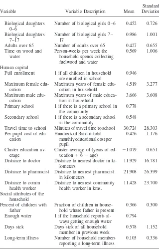
Table 4
Description of Child-Level Sample Variables for School-Age Children in Black South African Households
Standard
Variable Description of Variable Mean Deviation
Enrollment 1 if child is currently enrolled 0.900 0.301
Fostering characteristics
Foster-sibling 1 if child has a foster sibling 0.254 0.435
Present
Child fostered to close kin 1 if a foster child hosted by a close relative 0.148 0.355 Child fostered to remote kin 1 if a foster child hosted by a distant- or non-relative 0.016 0.124
Fostered-in girl 1 if the child is a girl and a foster child 0.081 0.273
Child characteristics
Age Age of child in years 11.666 3.176
Female 1 if a girl 0.501 0.500
Biological father present 1 if the child’s biological father is present 0.541 0.498 Household income and education characteristics
Maximum female education Maximum years of female education in household 5.416 3.734 Maximum male education Maximum years of male education in household 4.198 4.003
Log per capita Log per capita permanent income (expenditure) 5.337 0.698
Income
Pension income Exogenous pension income 1.821 6.920
Land size Hectares of cropland to which the household has access 0.465 4.587 Time on wood and water Person-weeks per week the household spends collecting 0.687 1.147
Zimmerman
573
Household demographic characteristics
All children 0–6 Number of children 0–6 in the child’s household 1.151 1.243 All female children 7–17 Number of girls 7–17 in the child’s household 1.563 1.180 All male children 7–17 Number of boys 7–17 in the child’s household 1.560 1.215 Adults over 65 Number of adults over 65 in the child’s household 0.451 0.665 Educated adult women Number of adult women in the child’s household with⬎ 0.491 0.803
7 years education
Uneducated adult women Number of adult women in the child’s household with 0.426 0.638
ⱕ7 years education
Educated adult men Number of adult men in the child’s household with⬎7 0.352 0.686 years education
Uneducated adult men Number of adult men in the child’s household withⱕ7 0.232 0.493 years education
Days sick Day sick of all household member in previous week 0.547 1.048
Long-term illness 1 for each household member reporting a serious long- 0.115 0.360 term illness
Community characteristics
Primary school 1 if there is a primary school in the community 0.799 0.401 Secondary school 1 if there is a secondary school in the community 0.562 0.496
Travel time to school Minutes of travel time to school 31.297 27.768
574 The Journal of Human Resources
considerations play a major role in fostering decisions and that fostering is a useful institution for building human capital.
The second hypothesis examines the extent to which fostering-in children arises out of a need for domestic labor, by testing the sign and significance of several of the coefficients. Under the domestic labor hypothesis, we would expect that the pres-ence of more men (M0) in a household increases the demand for home-produced
goods and increases the shadow value of domestic labor, thereby increasing the de-mand for foster children, and reducing the likelihood of enrolling them in school. We would expect both greater household assets (A) and greater exogenous income (R) to raise the marginal productivity of labor in home production, and therefore to increase the demand for foster children. The higher marginal productivity would tend to decrease the probability of enrollment, but greater assets or income would also generate a wealth effect tending to increase enrollment so that the net effect is ambiguous. The effect of the number of women (W0) in the household would be
stratified by their educational level. The presence of more educated women would increase the demand for domestic labor, thereby increasing the demand for foster children. The presence of more uneducated women, who in South Africa have limited income-earning capacity outside the household (May 1996), would tend to lower the demand for foster children, by lowering the marginal productivity of labor in home production. For the same reason, more uneducated women would tend to in-crease the probability of enrollment. Finally, more biological children (Nc) would
tend to lower the demand for foster children.
If fostering is indeed related to a demand for domestic labor, we would expect that, in response to fostering-in, households might reallocate existing labor at least in part toward greater market work. If so, fostering-in households would have higher cash income per capita as a result of the fostering decision, ceteris paribus. This hypothesis is tested via the coefficient on predicted fostering in the income regression (Equation 13). For similar reasons, we might expect that fostering-in, by releasing biological offspring from domestic labor, would enhance the probability of biological children being enrolled in school. We test this hypothesis in a schooling regression, by examining the significance of the coefficient on a variable indicating whether a child lives with biological parents who have fostered-in another child. If this coeffi-cient is positive, it would suggest that fostering does respond to a need for domestic labor, although this need arises out of a desire on the part of parents to send their own children to school.
In Hypothesis 5–7 we turn to the effects of fostering on the foster children’s school enrollments through three kinds of comparisons: a ‘‘Cinderella effect’’ comparison, a ‘‘migration effect’’ comparison, and a comparison of the total effect of fostering. In Hypothesis 5, we test the Cinderella effect, that is, whether foster children are less likely than biological children to be enrolled in school, controlling for other, observable child and household characteristics. A negative coefficient on foster child status will constitute at least circumstantial evidence of a Cinderella effect, and a statistically insignificant coefficient will suggest that we cannot reject the null hy-pothesis that there is no Cinderella effect. However, it is also possible that unobserv-able child characteristics are determinants both of school enrollment and of the fos-tering decision.
Zimmerman 575
or on their levels of discipline or potential. Indeed, the only relevant information on the children is their age and gender. Nor is there any data at all on the biological family of fostered-in children. Accordingly, it is not possible to control for such unobservable characteristics through instrumental variables. As a result, the results on the Cinderella effect must be treated with caution.
For example, Silk (1987) suggests that one reason boys in particular are fostered out is to enhance their discipline, and Goody (1982) reports that ‘‘difficult and proud’’ children are likely candidates to be fostered. If bad behavior at home is indeed a reason for fostering-out, and if—as seems reasonable—it is also a determi-nant of dropping out of school, then a negative coefficient on foster status in the school enrollment equation will not be indicative of a Cinderella effect. The opposite is also possible: if fostering-out is associated with some unobservable child charac-teristic that is also associated with greater school enrollment, then a finding of no Cinderella effect might be spurious. It should be noted, however, that there is little evidence in the anthropological literature to suggest that children with high potential are systematically fostered out. The choice of child to foster corresponds to gender considerations [for example, girls are not fostered to their mother’s brothers (Silk 1987)], traditional norms [the second-born child is often fostered (Silk 1987)], and the disciplinary motives cited earlier.
The second comparison of the effects of fostering on children is between the en-rollment rates of children in predicted fostering-in and fostering-out households. This comparison estimates the ‘‘migration effect,’’ that is, the contribution to a child’s enrollment probability of moving from the biological household to the foster house-hold. If fostering occurs in part to improve the human capital of children, we would expect the migration effect to be positive. Unfortunately, no data were collected on fostering-out households, that is, on biological children who live elsewhere. Data were collected, however, on the number of times each of the adult women in the household had given birth, the age of these women, and the number of children still living in the household. Using this information, it is possible to construct an indirect measure of whether the mother has fostered out children. Starting with the full sam-ple of black households, the number of living children of each woman younger than age 36 in the household is subtracted from the number of times she has given birth. If the resulting number is positive, it is assumed that she has fostered some of her children to other households. This approach, though clearly imperfect, is the best measure available in this data set, and it has been used in other studies of fostering (Page 1989).
576 The Journal of Human Resources
On the other hand, a positive net impact of fostering would suggest that the institution of fostering is a highly adaptive response to the multiple market imperfections and resource constraints of low-income areas.
V. Determinants of Fostering among South African
Blacks
Results of the household-level outcomes, estimated using the full sample of black households with school-age children, appear in Table 2. The first two columns of Table 2 present two versions of the probit estimates of fostering-in (Equation 10), first under the specification usfostering-ing the predicted enrollment vari-able, and then under the specification of the long-regression. The third column presents the probit estimates of a household fully enrolling its children, where the dependent variable is as described in the previous section. To facilitate interpre-tation, the parameter estimates of the probit models are presented as the marginal incremental change in the probability of fostering or full enrollment associated with a change in the regressor, rather than as the raw coefficients. The final column presents estimates of Equation 13, the log-income of the household per adult equivalent member.
Zimmerman 577
The equation used to predict whether households fully enroll their children is presented in Column 3 of Table 2. The pseudo-R2 of this regression, is 0.24, indicat-ing a modestly high degree of correlation between the instruments and the outcome. The second column of Table 2 presents a single-equation approach, in which the fostering regression includes the exogenous variables used to predict enrollment. These variables are now for the most part insignificant. The one exception is the cluster average of educational attainment, which is significant andnegativelyrelated to the probability of fostering in. This is not the result one would expect if a major motivation for fostering were to enhance school enrollment. However, it should be noted that this result is not necessarily inconsistent with the schooling motivation, since it is possible that foster children come from communities with yet lower levels of educational attainment. The coefficients on the numbers of educated and unedu-cated adult men and women in the household are also no longer significant. The remaining significant coefficients—on numbers of old people, on biological children aged 7–17, and on days sick—could be construed to support either the domestic labor hypothesis or the human-capital hypothesis, but in either case, the evidence is somewhat weak.6
The final column of Table 2 presents results of a regression of household income on many of these same variables, in addition to fostering status (Equation 13). Vari-ables that reflect the local environment, such as the distance to services and the time spent collecting wood and water, are excluded from this equation, because such variables do not enter the household’s income function (Equation 13). The coefficient on fostering-in is negative and statistically significant, although not especially large. (The mean for the dependent variable is 5.5.) If fostering-in were a way of gaining access to domestic labor to free up households for market work, then one would expect fostering-in to be positively associated with higher incomes, other things equal. This does not appear to be the case.
These results are somewhat at odds with those of Ainsworth’s (1996) study of fostering in Coˆte d’Ivoire. She regresses the fostering-in decision on a set of variables that includes the number of adult women and men in the household. Her regression shows positive coefficients on women and men, with higher coefficient values for women. She infers from this result that the demand for domestic labor is driving the decision to foster in children. The result of a positive and significant coefficient on adult women and men, however, is also consistent with a quite different hypothe-sis, namely that larger households are better able to take care of an additional mem-ber, both financially and in terms of time allocation. In any event, such results do not generally obtain in this sample.
The lack of strong support for the hypothesis of fostering as a demand for domestic labor or as a human-capital investment motive may be due in part to the pooling of fostering of both boys and girls of all ages. Table 3 presents the results for fostering-in by age and gender of the foster child, usfostering-ing the two-stage specification, that is, with predicted enrollment included in a probit of whether a household has
578 The Journal of Human Resources
in a child. (Conclusions do not differ when the single-equation approach is used.) Again, the sample is the full sample of Black households with children, and the dependent variables for the four regressions reported are whether the household has fostered-in a young girl, whether it has fostered-in an older girl, whether it has fos-tered-in a young boy, and whether it has fostered in an older boy. This is a modifica-tion of Equamodifica-tion 10. As with the pooled regression, predicted enrollment is correlated with fostering-in for most of the age/gender categories, with the exception of young boys. In the regressions on fostering-in girls, the coefficients on the time spent col-lecting wood and water is now significant, and larger and more significant for older girls, and not significant or large for boys. This result provides support for the hy-pothesis that the fostering-in of girls is a response to the demand for domestic labor. As before, however, foster girls—or foster boys—do not seem to be fostered-in to households with more land or with more young children. Moreover the coefficients on the number of adults in the household are not in general better predictors for the fostering-in of girls than the fostering-in of boys. To the extent that fostering-in corresponds to a demand for domestic labor, therefore, it would appear to arise as much out of the household’s isolation and lack of services as out of its demographic structure.
To the extent that girls are fostered-in for their value as domestic laborers, one might expect girls to be fostered in greater numbers than boys. This is not the case in these data: 13.59 percent of girls are fostered, and 13.68 percent of boys. (This difference is not statistically significant.)
The results of the fostering-in regressions at the household level can be summa-rized as follows. There is some evidence that is consistent with different hypotheses in the anthropological literature about the reason for fostering-in children: that it is both a response to a need for domestic labor and that it is way of improving the opportunities to build social ties and to invest in the human capital of children. There is somewhat more support for the hypothesis that fostering-in of older girls, in partic-ular, occurs out of a demand for domestic labor among isolated households that lack electricity and running water, although the evidence is limited, and is not statistically or economically strong. Finally, households that foster-in children do not appear to have higher incomes because of it. These results are consistent with the anthropologi-cal evidence of fostering as a social norm, and with Ben Porath’s conception of social norms as involving a network of give-and-take, which is broadly reciprocal without implying definite or equal bilateral exchanges.
VI. The Effects of Fostering on Human Capital
Investment in Children
Zimmerman 579
a comparison between enrollment rates of actual foster children and what those en-rollment rates would have been if the children had not been fostered.
Table 5 presents the results of probit regressions of children’s enrollment (mea-sured as a binary variable for individual children) on household-level, community-level and child-specific variables (Equation 11 above). The full sample includes all 8,627 school-age Black children, with subsamples as indicated in the table. The results are quite consistent across the three subsamples of girls, rural children, and rural girls. Several foster-related variables used are worth defining. A binary variable ‘‘foster-sibling presents’’ takes the value of 1 if the child is living with his or her biological parent(s), who have also taken in a foster child (zero otherwise). Two indicator variables represent foster child status: one for children who have been fostered to a close relative (grandparent, uncle or aunt, or brother or sister: 90 percent of the foster children) and another for children who have been fostered to a distant relative (cousin, brother-in-law, sister-in-law: 10 percent of the foster children). The omitted category is children living with their biological parents. Contrary to the prediction of Becker’s model, there is no Cinderella effect for children fostered to a close relative: the estimate of marginal effect of close-kin fostering is not signifi-cant. This result suggests that South African households treat foster children as they do their own children in terms of human capital investment when the child is a relative. Further strengthening this interpretation is the result for foster siblings of foster children (that is, children living with their biological parents, when those par-ents have taken in a foster child), whose enrollment rates are no better for having foster children in the household than for children living with their biological parents with no foster children present. The hypothesis that households foster in children to take over domestic chores from biological children, thereby freeing them up to attend school, receives no support here.
The previous section found some evidence that girls are fostered-in in part because of their ability to supply domestic labor to the foster household. The coefficient on foster girls in these regression is negative, but insignificant, suggesting that even for foster girls there is no Cinderella effect. These results, moreover, hold up well in a subsample of the population of children fostered to rural households (where one might expect a greater domestic labor workload) and also among girls fostered to rural households. Moreover, these results hold when the sample is broken down into three age categories (7–9, 10–14, 15–17).7
The Cinderella effect is, however, observable among the small number of children who are fostered to remote relations or to nonkin. Other things equal, these children are 5 percent less likely to attend school than children living with their biological parents. Of course, causal interpretations should be pursued with caution, since it is possible that the children who are fostered to remote kin may be more likely to have unobservable characteristics that predispose them not to attend school.
The last column of Table 5 presents a fixed-effects logit model, again with the dependent variable being a binary measure of enrollment measured for individual children. (Here the odds ratios are presented rather than the logit coefficients). The fixed-effects specification imposes several limits on the sample. Only those children
580
The
Journal
of
Human
Resources
Table 5
Child-Level Regressions of School Enrollment Among Children in Black South African Households
All Girls Rural Rural Girls Fixed-Effects
(Probit) (Probit) (Probit) (Probit) (Logit)
Marginal Marginal Marginal Marginal Odds
Effect |t| Effect |t| Effect |t| Effect |t| Ratio |t|
Foster-sibling present 0.001 (0.08) ⫺0.012 (1.32) 0.000 (0.02) ⫺0.017 (1.34)
Child fostered to close kin 0.012 (1.57) ⫺0.008 (0.89) 0.009 (0.89) ⫺0.016 (1.17) 0.490 (0.155)* Child fostered to remote kin ⫺0.051 (2.29)* ⫺0.067 (3.13)** ⫺0.071 (2.26)* ⫺0.091 (2.89)** 0.125 (0.075)**
Fostered-in girl ⫺0.020 (1.64) ⫺0.018 (1.13) 2.196 (0.781)*
Female 0.009 (1.86) 0.008 (1.23) 1.210 (0.191)
Biological father present 0.011 (2.07)* 0.009 (1.54) 0.012 (1.74) 0.009 (1.05)
Maximum female education 0.003 (3.39)** 0.002 (2.22)* 0.003 (3.15)** 0.004 (2.43)*
Maximum male education 0.001 (1.46) 0.000 (0.33) 0.003 (2.36)* 0.001 (0.69)
Redicted income 0.028 (2.21)* 0.013 (0.93) 0.041 (2.40)* 0.019 (0.92)
Pension income 0.001 (1.38) 0.001 (1.17) 0.001 (0.76) 0.001 (1.03)
Land size 0.000 (2.24)* ⫺0.003 (0.79) ⫺0.001 (2.30)* ⫺0.003 (082)
Time on wood and water 0.001 (0.46) 0.000 (0.13) 0.002 (0.80) 0.000 (0.02)
Zimmerman
581
All girls 7–17 0.005 (2.15)* 0.006 (2.27)* 0.005 (1.71) 0.007 (1.80)
All boys 7–17 0.001 (0.28) 0.004 (1.66) 0.002 (0.71) 0.006 (1.72)
Adults over 65 0.002 (0.45) 0.000 (0.03) 0.002 (0.38) 0.002 (0.34)
Educated adult women 0.004 (0.87) 0.010 (1.95) 0.005 (0.85) 0.006 (0.86)
Uneducated adult women ⫺0.010 (2.56)** ⫺0.016 (3.78)** ⫺0.012 (2.69)** ⫺0.023 (4.07)**
Educated adult men 0.004 (0.77) 0.001 (0.18) ⫺0.002 (0.26) ⫺0.005 (0.41)
Uneducated adult men ⫺0.007 (1.62) ⫺0.007 (1.42) ⫺0.005 (0.77) ⫺0.010 (1.27)
Days sick 0.003 (1.03) 0.004 (1.46) 0.002 (0.69) 0.004 (0.99)
Long-term illness ⫺0.026 (3.39)** ⫺0.026 (3.07)** ⫺0.031 (2.95)** ⫺0.028 (2.08)*
Primary school nearby 0.021 (2.16)* 0.016 (1.48) 0.016 (1.18) 0.010 (0.67)
Secondary school nearby ⫺0.001 (0.08) 0.003 (0.40) 0.003 (0.30) 0.008 (0.77)
Travel time to school 0.002 (8.28)** 0.002 (5.96)** 0.002 (7.31)** 0.002 (5.38)**
Per-pupil cost of education 0.021 (3.69)** 0.017 (2.51)* 0.019 (2.26)* 0.014 (1.45) Cluster-average education 0.027 (5.57)** 0.018 (3.44)** 0.035 (5.13)** 0.026 (3.11)**
attained
Enough water ⫺0.011 (1.77) ⫺0.009 (1.42) ⫺0.016 (2.16)* ⫺0.011 (1.39)
Observations 8,627 4,319 6,351 3,224 1,558
Number of households 465
Pseudo R-squared 0.27 0.29 0.26 0.27
Chi2 (df ) 737.88 (46) 467.46 (44) 689.85 (44) 372.81 (42) 392.69 (14)
Constant, Urban/Rural, Regional & Age Dummies: Included but not reported Absolute value of t-statistics in parentheses
582 The Journal of Human Resources
are included who are co-resident with at least one foster or biological sibling, and only those households are included in which there is a difference among children in enrollment status. As a result there are only 1,558 children from 465 households in this analysis, as opposed to 8,627 children from 3,693 households in the full sample. Among children living in households where at least one, but not all, children are enrolled, children fostered to a relative are about half as likely as the biological child to be the one attending school.8However, all of this effect is due to
fostered-in boys, sfostered-ince fostered-fostered-in girls are twice as likely to be the one attendfostered-ing school in these households. For their part, children fostered to remote kin are about one-eight as likely to be the one attending school. Taken together, the fixed-effects specification largely corroborates the finding of no Cinderella effect for girls, but it does find a Cinderella effect for boys. This result is particularly intriguing given that in the household-level regressions of the previous section on fostering-in, it was the fostering-in of girls that seemed to respond somewhat more to domestic labor needs.
To further analyze these effects, Table 6 presents results of OLS regressions of the time children spend collecting wood and water (Equation 12), for the full sample of all children, with separate analyses for girls, rural children, and girls in rural areas. Two results are quite striking: not only do foster children spend no more time collecting wood and water than children living with their biological parents, but children living with their biological parents in rural areas spendmoretime collecting wood and water when a foster child is present. This result probably does not arise out of household selection, since, as Table 3 revealed, among households in rural areas the time spent collecting wood and water was not related to the decision to foster-in a child. Instead it would appear that households are genuinely devoting resources to the foster child.
Table 7 displays the results for the second and third comparisons: the migration effect, and the net impact of fostering. For each comparison there is an issue of the appropriate counterfactual group. To assess the migration effect, for example, chil-dren in typical fostering-out households may be compared either to chilchil-dren in typi-cal (that is, predicted) fostering-out households, or to those in actual fostering-out households. Using children in actual fostering-out will pick up unobservable house-hold effects that no doubt also influence the fostering decision, such as unreported adult illness or other family crises. At the same time, however, the act of fostering-out one or more children may tend to alleviate the pressure on the remaining child-ren, so that a comparison between fostered-out children remaining children would understate the true value of fostering. On the other hand, comparisons with pre-dicted fostering-out households suffer from the downward bias in estimating the difference in that households that are predicted to foster out do not all suffer from the unobserved crises or other household-specific effects that help motivate the fos-tering-out decision. Comparisons of the enrollments of foster children to the enroll-ments of children both in predicted out households and actual fostering-out households are therefore reported in Table 7. Both of these comparisons are also
Zimmerman 583
subject to possible bias arising from potentially nonrandom selection of children to foster. For this and other reasons, these comparisons should be interpreted with caution.
Predicted fostering-out households were identified as follows. First, a probit re-gression of fostering-out (as defined in Section IV) was run, and, for all households, the predicted probability of fostering-out was obtained. Because 7 percent of house-holds foster-out children, househouse-holds were defined as being predicted to foster-out children if their estimated probability of doing so was above the 93rd percentile for the sample. In this way, the number of predicted fostering-out households is equal to the number of actual fostering-out households. A similar approach was used to identify predicted fostering-in households, and households that were predicted to foster-in a close relative. For all of these prediction estimations, results are not re-ported here, but are available from the author. The mean enrollment rates were as-sessed for each of the categories of fostering-status identified in this way.
The migration effect, presented in Rows 5 and 6 of Table 7, is large: the move of a child from the biological household to a foster household results in a 3–4 per-centage-point increase in the probability of school enrollment, depending on the comparison used. Put differently, the migration effect of fostering reduces the risk of not attending school by approximately 25 percent. These results are broadly con-sistent for different subsamples of the population and for both specifications of the counterfactual. A major exception is in the comparison of enrollments of children over 14 between predicted fostering-in and predicted fostering-out households, in which the migration effect is shown to benegative: fostering-in households are 2 percentage points less likely to enroll children than fostering-out households. This result does not hold for the comparison between predicted fostering-in and actual fostering-out households, however, nor for any of the other subpopulations.
The net impact of fostering, presented in Rows 9 and 10 of Table 7 is also mean-ingful: the institution of fostering allows parents to boost their child’s chances of enrollment again by a 2–3 percentage-point increase. The net impact of fostering im-plies a risk reduction of either 14 percent or 22 percent, depending on the counter-factual. Again, these differences are robust in several relevant subsamples, with the exception again being children older than 14, this time in the comparison of actual foster children to children in actual fostering-out households, that is, their biological siblings. While it is risky to second-guess the magnitude or even the direction of bias introduced by unobservables, it will be remembered that the anthropological evidence cited in Section II suggests that children with disciplinary problems are often fostered out to improve their behavior. If so, the children left behind (that is, children in actual fostering-out households) are a selected sample of children who are more likely to attend school due to unobservable characteristics of their behavior. In that case, it would be plausible that the finding of a negative impact of fostering in this one comparison could be due to the effects of such unobservable characteristics. It should be noted that in general the benefits of fostering are large for all children, and are as pronounced for girls as for boys. This result is consistent of earlier findings of no gender bias in the way foster girls are treated, relative to foster boys.
584
The
Journal
of
Human
Resources
Table 6
Child-Level Regressions of Time Spent Collecting Wood and Water Among Black South African Households
Fixed-Effects
All Girls Rural Rural Girls Analysis
βˆ |t| βˆ |t| βˆ |t| βˆ |t| βˆ |t|
Foster-sibling present 0.152 (1.85) 0.176 (1.06) 0.222 (2.03)* 0.251 1.19
Child fostered to close kin ⫺0.028 (0.35) 0.122 (0.88) ⫺0.069 (0.62) 0.135 (0.72) ⫺0.207 (1.03)
Child fostered to remote kin 0.131 (0.53) 0.452 (1.29) 0.187 (0.56) 0.759 (1.53) 0.420 (1.02)
Fostered-in girl 0.209 (1.46) 0.341 (1.76) ⫺0.070 (0.33)
Female 1.04 (8.77)** 1.389 (9.42)** 1.197 (14.07)**
Biogical father present ⫺0.13 (2.11)* ⫺0.227 (2.33)* ⫺0.145 (1.73) ⫺0.272 (2.14)*
Predicted income 0.774 (5.33)** 1.177 (4.59)** 1.268 (6.38)** 1.902 (5.44)**
Pension income ⫺0.004 (3.95)** ⫺0.005 (2.61)** ⫺0.008 (0.75) ⫺0.019 (1.16)
Land size ⫺0.005 (4.03)** 0.030 (0.55) ⫺0.007 (4.92)** 0.035 (0.64)
Time on wood and water 1.112 (12.65)** 1.728 (10.71)** 1.129 (12.88)** 1.751 (11.01)**
All children 0–6 ⫺0.021 (0.76) ⫺0.059 (1.18) ⫺0.008 (0.24) ⫺0.042 (0.69)
All girls 7–17 ⫺0.128 (3.86)** ⫺0.141 (2.64)** ⫺0.163 (4.03)** ⫺0.181 (2.68)**
All boys 7–17 0.026 (0.90) 0.020 (0.36) 0.023 (0.65) 0.013 (0.19)
Adults over 65 0.125 (2.68)** 0.145 (1.68) 0.199 (2.88)** 0.241 (1.91)
Zimmerman
585
Educated adult men ⫺0.042 (1.10) ⫺0.044 (0.70) ⫺0.073 (1.36) ⫺0.046 (0.48)
Uneducated adult men 0.122 (2.18)* 0.269 (2.53)* 0.212 (2.76)** 0.414 (2.90)**
Days sick 0.006 (0.22) 0.016 (0.30) ⫺0.003 (0.008) 0.008 (0.12)
Long-term illness 0.093 (0.98) 0.318 (1.77) 0.122 (0.91) 0.383 (1.56)
Primary school nearby ⫺0.029 (0.41) ⫺0.070 (0.58) ⫺0.037 (0.40) ⫺0.133 (0.81) Secondary school nearby 0.028 (0.43) ⫺0.086 (0.75) 0.046 (0.59) ⫺0.030 (0.20)
Travel time to school 0.001 (0.84) 0.001 (0.74) 0.001 (0.79) 0.001 (0.66)
Per-pupil cost of education ⫺0.023 (1.76) ⫺0.031 (1.22) ⫺0.037 (1.56) ⫺0.034 (0.94) Cluster-average education 0.070 (1.72) 0.080 (1.04) 0.125 (2.39)* 0.185 (1.74)
attained
Enough water ⫺0.076 (0.68) ⫺0.13 (0.64) ⫺0.101 (0.84) ⫺0.193 (0.90)
Observations 8,514 4,260 6,296 3,195 7,330
Number of households 2,467
Within: 0.11
R-squared 0.26 0.37 0.27 0.37 Between: rho⫽.344
0.04 Overall:
0.08 Absolute value oft-statistics
in parentheses
586
The
Journal
of
Human
Resources
Table 7
Comparisons of Schooling Effects of Fostering Among Black South Africans
Children Fostered to Close
All Relatives Over 14 Girls Boys
1. Probability of enrollment for full sample 0.900 0.889 0.910 0.890
(0.006) (0.009) (0.006) (0.007)
Migration Effect
2. Probability of enrollment for children in predicted fostering-in 0.892 0.890 0.873 0.906 0.878
households (0.010) (0.010) (0.019) (0.011) (0.013)
3. Probability of enrollment for predicted fostering-out households 0.869 0.879a 0.900 0.888 0.850
(0.020) (0.016) (0.032) (0.021) (0.025) 4. Probability of enrollment in actual fostering-out households 0.851 0.851a 0.814 0.865 0.839
(0.019) (0.019) (0.042) (0.024) (0.022) 5. Differences in probability of enrollment between predicted 0.032 0.029 ⫺0.022 0.024 0.041
Zimmerman
587
6. Differences in probability of enrollment between predicted 0.037* 0.032 0.042 0.036b 0.036b
fostering-in households and actual fostering-out households: 2–4 (0.022) (0.022) (0.044) (0.027) (0.027) 7. Change in risk of not attending school due to migration:
• Using predicted fostering-out HH: (6)/[1–(4)] ⫺24.83% ⫺21.48% ⫺22.58% ⫺26.67% ⫺22.36% • Using actual fostering-out HH: (5)/[1–(3)] ⫺24.43% ⫺23.97% ⫹22.00% ⫺21.43% ⫺27.33% Net Fostering Impact
8. Probability of enrollment for foster children 0.884 0.898 0.846 0.897 0.872 (0.010) (0.010) (0.022) (0.013) (0.014) 9. Difference in probability of enrollment between actual foster 0.018 0.033 ⫺0.073* 0.015 0.023
children and children in predicted fostering-out households: 8–3 (0.021) (0.021) (0.039) (0.024) (0.028) 10. Difference in probability of enrollment between actual foster 0.033 0.047** 0.009 0.032 0.037
children and actual fostering-out households: 8–4 (0.022) (0.022) (0.045) (0.026) (0.029) 11. Change in risk of not attending school: net fostering impact:
• Using predicted fostering-out HH: (10)/[1–(4)] ⫺22.15% ⫺31.54% ⫺4.84% ⫺23.70% ⫺22.98% • Using actual fostering-out HH: (9)/[1–(3)] ⫺13.74% ⫺27.27% ⫹73.00% ⫺13.39% ⫺15.33%
a. Since it is not possible to predict whether a household will foster a child to a close relative as opposed to a distant relative, this is the same as the ‘‘All’’ Column. b. Sic.