Parental Problem-drinking and Adult
Children’s Labor Market Outcomes
Ana I. Balsa
a b s t r a c t
Current estimates of the societal costs of alcoholism do not consider the impact of parental drinking on children. This paper analyzes the consequences of parental problem-drinking on children’s labor market outcomes in adulthood. Using the NLSY79, I show that having a problem-drinking parent is associated with longer periods out of the labor force, lengthier unemployment, and lower wages, in particular for male respondents. Increased probabilities of experiencing health problems and abusing alcohol are speculative forces behind these effects. While causality cannot be determined due to imprecise IV estimates, the paper calls for further investigation of the intergeneration costs of problem-drinking.
I. Introduction
An important avenue of research in economics involves the identifi-cation and measurement of the economic costs of alcoholism. In most cases, the scope of this research has been limited to studying the consequences directly asso-ciated with the problem-drinking subject: for example, productivity losses, health care costs, and other costs directly resulting from the criminal activities of the sub-ject. Less is known, however, about indirect economic costs of alcoholism such as, for instance, the costs that one family member’s drinking inflicts upon other family members.
Ana I. Balsa is a visiting scientist with the Health Economics Research Group (HERG) at the University of Miami and a visiting professor at the University of Montevideo, Uruguay. Financial assistance for this study was provided by the National Institute on Alcohol Abuse and Alcoholism (grant number R01 AA13167). The author gratefully acknowledges comments and suggestions by attendants to the HERG research meetings, three anonymous referees, William Russell for editorial assistance, and Jamila Wade and Colleen Trifilo for research assistance. The results, opinions, and positions presented in this paper reflect the views of the author alone and do not necessarily represent those of the University of Miami or the National Institute on Alcohol Abuse and Alcoholism. The data used in this article can be obtained beginning October 2008 through September 2011 from Ana I. Balsa, Ph.D., University of Miami, Sociology Research Center, 5665 Ponce de Leon Boulevard, Flipse Building room 122, Coral Gables, FL 33146-0719, U.S.A.; abalsa@miami.edu.
[Submitted January 2006; accepted June 2007]
ISSN 022-166X E-ISSN 1548-8004Ó2008 by the Board of Regents of the University of Wisconsin System
This paper takes advantage of the 1979 cohort of the National Longitudinal Survey of Youth (NLSY79), a rich, nationally representative longitudinal data set, to analyze the economic effects of parental problem-drinking on children. Specifically, the pa-per focuses upon labor market outcomes of adult children of alcoholics, including labor force participation, unemployment, and wages. Results are suggestive of inter-generation costs of problem-drinking, but the analysis cannot reach definite conclu-sions about the causality of the effects.
Alerting the public to the consequences of parental drinking has significant impli-cations for public policy. In general, the costs that children of alcoholics have to bear because of parental alcoholism are not considered when evaluating the economic consequences of alcohol abuse, nor are they taken into account when designing rel-evant interventions. The current paper sheds new light on the economical signifi-cance of parental problem-drinking and emphasizes the importance of considering these costs when designing, evaluating, and funding interventions.
Section II surveys the previous literature on the effects of parental alcoholism in children and provides some insight on the pathways through which alcohol misuse by a parent could affect a child’s labor market outcomes at adulthood. A description of the NLSY79 data, the variables used in the analysis, and the estimation methods is provided in Section III. Section IV reports the results and checks for robustness using alternate methodologies. In Section V, results are discussed and a conclusion is offered.
II. Background and Significance
Most of the previous research on children of alcoholics has been per-formed in the fields of clinical psychology and family medicine. Findings suggest that children of alcoholics are at higher risk than other children for depression, anx-iety disorders, problems with cognitive and verbal skills, and parental abuse or ne-glect during childhood (NIAAA 2000). The bulk of the research focuses on the short- to medium-term sequels that parental alcohol misuse has on children. Al-though many studies relate parental alcoholism to higher likelihood of children engaging in problematic drinking, it remains unclear whether parental problem-drinking leaves a long-term economic imprint on children.
Connell and Goodman (2002) identify four mechanisms that relate parental alco-hol abuse to children’s adverse outcomes: (1) genetics; (2) complications during pre-natal development; (3) exposure to the parent’s behavior and knowledge; and (4) environmental stressors such as economic pressure, marital conflict, and disruption that are more common in a home with an alcoholic or problem-drinking parent. By affecting mental and physical health, levels of IQ, learning capabilities, substance use patterns, and attitudes in general, each of these mechanisms can shape a child’s future labor market success.
The higher propensity of children of alcoholics to develop drinking problems is a first pathway that could relate parental drinking to children’s labor market outcomes at adulthood. A family history of alcoholism has been identified as a critical predis-posing factor of high risk for alcohol dependence at later ages (Jennison and Johnson 1998; Windle 1996; Jennison and Johnson 2001). Findings of twin and adoption
studies have enhanced the understanding of genetic susceptibility to alcohol depen-dence (McGue 1997). Prevalence of alcoholism among first-degree relatives of indi-viduals suffering from alcoholism is 3–4 times greater than it is among the general population, while the rates are even higher among identical twins (Schuckit 1999). In addition, research shows that children of alcoholics develop expectations about the effects of alcohol by observing their parents’ drinking and may turn to alcohol as a means of alleviating other conditions (Ellis, Zucker, and Fitzgerald 1997). As with other behavioral conditions, the gene-environment interaction increases children of alcoholics’ risks of developing alcohol abuse or dependence. This higher predisposi-tion to misuse alcohol may affect labor market outcomes through its negative effects on human capital formation and employment. Yamada, Kendrix, and Yamada (1996), Chatterji and DeSimone (2005), and Koch and McGeary (2005) find that drinking in high school significantly reduces the probability of high school graduation. Williams, Powell, and Wechsler (2003) show that alcohol consumption in college has a nega-tive effect on GPA, which works mainly through a reduction in the hours spent study-ing. Booth and Feng (2002) and McDonald and Shields (2001) find that heavy drinking significantly increases the probability of unemployment and reduces the number of weeks worked among those employed. Other work, however, finds little role for alcohol in educational attainment (Dee and Evans 2003; Koch and Ribar 2001) or unemployment (Feng et al. 2001).
Prenatal exposure to alcohol is a second channel through which parental alcohol abuse can affect children’s productivity. The exposure of fetuses to high amounts of alcohol has been shown to have devastating effects on development. Fetal alcohol syndrome (FAS) has been associated with structural abnormalities, growth deficits, and neurobehavioral anomalies. Among other problems, children with FAS face defi-ciencies related to activity, attention, learning, memory, language, motor, and visuo-spatial abilities (see Mattson and Riley (1998) for a review of this literature).
productivity. Depression and other health conditions may decrease labor force partic-ipation, reduce attendance to work for those employed, and affect productivity and wages.
A final and more direct channel would consist in the need of an adult child to take time from school or work to take care of a parent with a drinking problem.
In sum, children of alcoholics face a number of constraints that condition their la-bor market outcomes in adulthood: a higher predisposition to misuse alcohol, a higher likelihood of congenital developmental problems, a stressful environment that leads to mental and possibly other health problems, and the burden of having to take care of a sick parent. The aim of this paper is to find evidence of the aggregate effect of these constraints on children’s labor market success.
III. Data and Methodology
A. The NLSY79The data used for this analysis is the National Longitudinal Survey of Youth 1979 (NLSY79). The NLSY79 is a nationally representative sample of 12,686 young men and women who were 14–22 years old when they were first surveyed in 1979. These individuals were interviewed annually through 1994 and are currently interviewed on a biennial basis. The NLSY79 cohort provides researchers with the opportunity to study a large sample of individuals representing American men and women born in the 1950s and 1960s and living in the United States in 1979. Labor market information includes the start and stop dates for each job held since the last interview, labor market activities (looking for work, out of the labor force) during gaps between jobs, hours worked, earnings, occupation, industry, benefits, and other specific job characteristics. In addition, the survey collects detailed information about personal and family characteristics, such as educational attainment, income and assets, health conditions that limit the ability to work, and use of alcohol and other substances.
B. Definition of Variables
1. Dependent variables
The analysis focuses on three indicators of labor market performance of children of problem-drinking parents at middle age: labor force participation, unemployment, and hourly wages. Rather than focusing on a single year, these measures are averaged across a period spanning six years (1996–20021) and four interviews. This implies that for individuals who were 14 years old in 1979, labor market performance is mea-sured during the period when they were between 31 and 37 years old. For those in the other extreme (aged 22 in 1979), the analysis considers labor market outcomes while in their late thirties and early-to-mid forties (39 to 45). Working with average meas-ures of outcomes across years has several advantages. First, it minimizes measure-ment error and the incidence of exogenous temporary shocks on labor market
1. Surveys were administered every two years in this period: 1996, 1998, 2000, and 2002.
outcomes. We are interested in the permanent impact of parental problem-drinking on the labor trajectories of their offspring in adulthood, and working with averages achieves this aim more effectively than considering single years. Second, it substan-tially reduces problems of missing observations due to nonresponse. If an individual responded to the survey in 1996 and 1998, but did not respond in 2002, we would still have a measure of labor market outcomes. Third, averaging across years circum-vents the problem of not observing a reservation wage. Because a relatively low pro-portion of individuals remain unemployed for six years in a row, we are more likely to observe the individual’s reservation wage. Also, we are more likely to observe individuals who participate intermittently in the labor force.
Labor force participationis measured as the average number of weeks per year the respondent was out of the labor force between 1995 and 2001. Note that because of the biennial nature of the survey, the measure only considers the average number of weeks of nonparticipation corresponding to the calendar years prior to the 1996, 1998, 2000, and 2002 surveys.2 Unemployment is defined as the average number of weeks per year the respondent was unemployed in 1995, 1997, 1999, and 2001. For the computation of hourly wages, only respondents that did not report self-employment in the 1996–2002 surveys are considered. Hourly wages in a particular year are measured as the ratio of total wage earnings to total hours worked in that year, adjusted to 2002 values using the Bureau of Labor Statistics CPI. A measure of hourly wage is averaged across the years 1995, 1997, 1999, and 2001, and outliers showing a wage per hour below $1 or above $300 are dropped from the regressions (76 observations less than $1 and eight observations more than $300). To normalize the distribution, the logarithm of the average hourly wage is computed.
2. Parental Problem-drinking
In 1988, the NLSY respondents were asked whether they had ever had any relatives who had been alcoholics or problem drinkers at any point in their lives and, if so, to indicate their relationship to each of these relatives. A dichotomous indicator for having had a problem-drinking parent is constructed on the basis of these questions. The measure considers both biological and nonbiological parents. The data offered the possibility of constructing separate indicators for a problem-drinking mother and a problem-drinking father. However, the small number of problem-drinking mothers (5 percent in the female sample and 3 percent in the male sample) raised concerns about the power of the data to achieve statistically significant estimates. In addition, it was very hard to find instrumental variables that were relevant predic-tors of a problem-drinking mother.
3. Demographics
The analysis adjusts for age—nine categories ranging from 14 to 22 years old in 1979—and for race/ ethnicity—White, Hispanic, Black, or Other. All analyses are run separately for male and female respondents.
2. While NLSY has information on the cumulative number of weeks out of the labor force since the last interview, dealing with these variables is confusing because of the different rates of responses and different interview dates.
4. State dummy variables
Thirty-nine different geographic dummies are constructed to indicate the state of res-idency of the respondent at age 14. Due to the low number of respondents in various states, a number of observations had to be aggregated into a single category. Includ-ing state dummy variables as controls contributes to isolate the effects of a problem-drinking parent from influences at the geographic level that can affect a respondent’s own propensity to drink as well as his/her human capital and labor market choices.
5. Other data
The relationship between a problem-drinking parent and an adult child’s labor mar-ket outcomes can be mediated by a number of factors, such as family and household characteristics during childhood, investment in education, health status, drinking tra-jectories, and family choices, among others. While none of these measures is incor-porated in the main analysis due to the inherent endogeneity, a descriptive account of such variables is presented in Table 5. Initial comparisons of these features among children of problem-drinking parents and other children can contribute to build hy-potheses about the pathways linking parental problem-drinking to children’s labor market outcomes.
C. Sample and Data Description
The sample used for this analysis excludes NLSY respondents from the military sam-ple, who were only surveyed up to 1984, as well as economically disadvantaged mi-norities of the supplemental subsample, who were not eligible for interview as of the 1991 survey. A total of 9,986 individuals were eligible for interview in 1996–2002. Of these, 9,028 responded to at least one of the four surveys administered between 1996 and 2002 (90 percent response rate). Among the remaining 9,028 observations, a total of 534 did not respond to the parental alcohol questions. The final sample has 8,494 observations, including 4,199 for males and 4,295 for females. Rates of partic-ipation in the 1996–2002 interviews do not differ across children of problem-drink-ing parents and other respondents.
Table 1 compares the means of the dependent variables and demographics across children of problem-drinking parents and other respondents. The statistics are shown separately for males and females. It is interesting to note that male respondents are less likely to answer the questions about parental drinking and less likely to report a problem-drinking mother or father than female respondents. Nineteen percent of male respondents report having had a problem-drinking parent, while the rate is 26 percent for females. This difference clearly indicates a reporting bias in the data. Regarding labor market outcomes, both male and female children of problem drinkers are more likely to be out of the labor force. Daughters of problem drinkers earn slightly lower hourly wages than other females. Parental problem-drinking is more prevalent in White families and less prevalent in African American families.
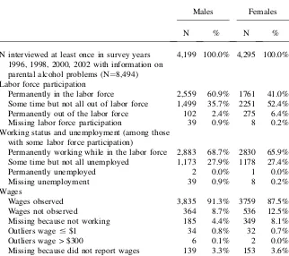
Table 2 describes in more detail the labor market outcomes for males and females. More than one third of male respondents and half of female respondents report at least one week out of the labor force during 1995–2001, and a few respondents stay permanently out of the labor force during the period (2.4 percent of men and 6.4 per-cent of women). Twenty-eight perper-cent of both men and women experience some
Table 1
Data Means, by Parental Problem-drinking Statusa
Male Respondents Female Respondents
Total N¼9,986b 5,034 4,952
Percentage responding questions about parental drinking 88.8% 90.6%
Percentage reporting problem-drinking parent 19.0% 26.1%
Percentage reporting problem-drinking mother 3.4% 5.2%
Percentage reporting problem-drinking father 17.3% 23.0%
Problem-drinking parent
No problem-drinking
parent
Problem-drinking parent
No problem-drinking
parent
N 851 3,618 1,169 3,315
Percentage interviewed at least once in 1996–2002 94.7% 93.8% 96.5% 95.5% Labor market outcomes
Weeks out of labor force (average 95, 97, 99,01) 7.408 4.889*** 12.549 11.576**
Weeks unemployed (average 95, 97, 99, 01) 2.292 1.981 1.652 1.651
Ln hourly wage (average 95, 97, 99, 01) 2.714 2.745 2.414 2.480***
Controls
Age 1979¼14 0.099 0.092 0.067 0.084**
Age 1979¼15 0.170 0.137** 0.139 0.131
Age 1979¼16 0.127 0.143 0.124 0.145**
Age 1979¼17 0.129 0.135 0.139 0.140
Age 1979¼18 0.120 0.146** 0.130 0.135
Age 1979¼19 0.102 0.119 0.134 0.124
460
The
Journal
of
Human
Age 1979¼20 0.114 0.103 0.121 0.103**
Age 1979¼21 0.115 0.098 0.124 0.114
Age 1979¼22 0.024 0.027 0.021 0.024
Non-Hispanic white 0.528 0.484** 0.526 0.485***
Hispanic 0.177 0.192 0.186 0.189
Black 0.282 0.313** 0.279 0.312**
Other race 0.013 0.011 0.009 0.013
Note: ** Difference between respondent with problem-drinking parent and respondent with no problem-drinking parent statistically significant at 5 percent; *** difference statistically significant at 1 percent.
a. Parental problem-drinking¼1 when respondent reported either a biological or nonbiological problem-drinking mother or father. b. Excludes NLSY79 respondents from the military sample and economically disadvantaged minorities of the supplemental subsample.
Balsa
unemployment in 1995–2001. Wages are not observed for 9 percent of the male and 12 percent of the female sample.
There are two sources of sample selection in the data: attrition and failure to an-swer the questions about alcohol problems in the family. Table 1A in the Appendix shows the mean differences between some of the variables in the sample used for the main analysis and variables in the other two samples. Those not interviewed in 1996– 2002 are more likely to belong to White, highly educated families and less likely to report a problem-drinking father at baseline, reducing concerns about attrition of the most severe cases. On the other hand, Hispanics and children raised in lower-income families are overrepresented among respondents who do not answer the parental al-cohol use questions. These individuals are more likely to be high school dropouts and show more weeks out of the labor force. While their rate of alcohol dependence is lower than that in the final sample, there is also a higher rate of nonresponse to the DSM-IV questions. Judging from the profile of this sample, it could be possible that parental alcoholism was more severe among these individuals. If this were the case, our results would be biased toward zero by failing to include the cases more affected by parental drinking.
Table 2
Labor Market Outcomes for Respondents Interviewed at Least Once in 1996–2002
Males Females
N % N %
N interviewed at least once in survey years 1996, 1998, 2000, 2002 with information on parental alcohol problems (N¼8,494)
4,199 100.0% 4,295 100.0%
Labor force participation
Permanently in the labor force 2,559 60.9% 1761 41.0%
Some time but not all out of labor force 1,499 35.7% 2251 52.4%
Permanently out of the labor force 102 2.4% 275 6.4%
Missing labor force participation 39 0.9% 8 0.2%
Working status and unemployment (among those with some labor force participation)
Permanently working while in the labor force 2,883 68.7% 2830 65.9%
Some time but not all unemployed 1,173 27.9% 1178 27.4%
Permanently unemployed 2 0.0% 1 0.0%
Missing unemployment 39 0.9% 8 0.2%
Wages
Wages observed 3,835 91.3% 3759 87.5%
Wages not observed 364 8.7% 536 12.5%
Missing because not working 185 4.4% 349 8.1%
Outliers wage#$1 34 0.8% 32 0.7%
Outliers wage > $300 6 0.1% 2 0.0%
Missing because did not report wages 139 3.3% 153 3.6%
D. Methodology
The equation of interest is of the form:
Yi¼a0+a1Ai+Age9ia2+Race9ia3+State9ia4+ei ð1Þ
whereYiis a labor market outcome andAiis an indicator for a problem-drinking
par-ent. Because family, household, and many individual characteristics are endogenous, only a set of purely exogenous dummies—age, race, and fixed effects for the respondent’s state of residency at age 14—are included as controls. The state dum-mies adjust the model for exogenous geographical influences that may shape an indi-vidual’s human capital and labor market opportunities. The choice of age 14 responds to the belief that many attitudes, including the respondent’s own propensity to drink, are forged during adolescence by the geographical environment. The idea is to isolate this environmental effect from parental influences due to alcohol misuse. In addition to estimating Equation 1 with ordinary least squares, the model is es-timated with alternative single equation techniques that better suit the particular out-come analyzed. In the case of count variables such as number of weeks out of the labor force and number of weeks unemployed, the model is reestimated using neg-ative binomial regressions. When the outcome of interest is hourly wages, which involves selection due to incidental truncation,3 the model is also estimated using a Heckman two-step regression. In the first stage, I estimate the likelihood of observ-ing the wage among all those respondobserv-ing to the survey. The wage regression is esti-mated next, adjusting for the selection implicit in the first stage. The exclusion restriction in the first stage is given by a variable constructed in 1979 that described the respondent’s level of impatience when completing the interview (as reported by the interviewer).
One problem with using single-equation regression to estimate Equation 1 is that omitted variables may be biasing the results. For example, exogenous negative shocks to the family (for example, a death of a family member) may increase the likelihood that a parent becomes a problem drinker and, at the same time, deteriorate the child’s mental health. Or an adverse economic period for the family could increase parental drinking and at the same time reduce the child’s possibilities of graduating from high school or attending college. These mental health limitations or economic adversities could have a long-term impact upon children’s productivity. It is also pos-sible that careless personalities could lead parents to drink rather than take care of their families. Inability to control for these or other latent variables might result in spurious associations between parental drinking and children’s long-term outcomes. Instrumental variables, if relevant and valid, can address this problem by restricting the analysis to those components of the main explanatory variable (Problem-drinking Parent) that are uncorrelated with the error term in Equation 1. The instruments cho-sen to predict a problem-drinking parent are (1) an indicator of a problem-drinking grandfather on the father’s side, (2) cigarette and beer excise taxes in the family’s state of residence at the time of the respondent’s birth, (3) cigarette excise taxes in the mother’s state of birth in 1947 (approximately 14 years prior to the respond-ent’s birth), and (4) a dummy variable indicating whether there were alcohol sales
3. Incidental truncation in this case is due to the fact that wages are only observed for people who work.
controls in the father’s state of birth in 1947.4The indicator of a problem-drinking grandfather was constructed on the basis of the same questions (1988 survey) used to define the parental problem-drinking indicator. Excise taxes were obtained from the Book of States (1947–64).
Cigarette and beer taxes are commonly used instruments in this type of analysis (French and Maclean 2006; Mullahy and Sindelar 1996; Chatterji and Markowitz 2001). Some researchers have criticized these instruments because they may be con-founded with attitudes at the geographic level. Such problem is minimized in this paper by including controls for the respondent’s state of residency at age 14 and by using policy variables that were in place 14 or more years before at the respondent’s state of residency and at the mother or father’s state of birth. Thus, we are exploiting the var-iation on excise taxes across time and across states (for those parents who moved).
Problem-drinking by other family members, such as grandparents, aunts, or uncles, are highly predictive of parental problem-drinking and have been used suc-cessfully in other related studies as instruments (French and Maclean 2006; Mullahy and Sindelar 1996). Problem-drinking by a grandfather is a valid instrument only if it affects a child’s labor market outcomes through paternal or maternal alcohol prob-lems. It seems unlikely that this familial instrument would be correlated with con-temporaneous shocks or other omitted variables that could simultaneously affect the children’s human capital and the parent’s drinking. It remains possible, however, that the influence of a problem-drinking grandfather on an adult grandchild works indirectly through other channels. Our analysis therefore recognizes that such an in-strument can mitigate but probably not completely eliminate biases arising due to endogeneity. For this reason, some sensitivity analyses are conducted using only al-cohol policy variables as instrumental variables. Unfortunately, alal-cohol policy vari-ables tend to be weaker instruments when considered on their own.
Instrument relevance is tested using theF-test of the joint significance of the ex-cluded instruments in a linear probability model predicting a problem-drinking par-ent. For each outcome of interest, overidentifying restrictions are tested using the HansenJstatistic (Hansen 1982).5I also run tests of subsets of the exclusion restric-tions to ensure that each of the instruments, including State policies and the family drinking history indicator, satisfy by themselves the orthogonality requirements. The
C-statistic or difference in Sargan test is used for this purpose (Hayashi 2000). Endogeneity is addressed using generalized method of moments (GMM). Tests of heteroskedasticity revealed that most of the models analyzed had heteroskedasticity
4. The mentioned alcohol and cigarette policies were selected from a more extensive data set that included spirit, beer, wine, and cigarette taxes, as well as other policies such as state controls of alcohol sales. These policies were collected for several time periods and geographic locations: (a) at the family’s state of resi-dency by the time of the respondent’s birth; (b) at the father’s state of birth approximately 14 years prior to the respondent’s birth; and (c) at the mother’s state of birth approximately 14 years prior to the respondent’s birth. Taxes in dollars were adjusted to 2002 values using the BLS CPI. The final set of instruments in-cluded those policies that achieved jointly the highest level of significance in the prediction of a problem-drinking parent.
5. The HansenJstatistic differs from the Sargan’s statistic in that it tests overidentifying restrictions under the assumption of heteroskedasticity. Note that failure to reject the hypothesis of no overidentification in any of these tests does not guarantee that the instruments satisfy the orthogonality requirements. Failure to reject could be due, for example, to low power in one or more of the instruments.
of unknown form and GMM is more efficient than two stages least squares (2SLS) in such situation. The GMM estimator solves:
gðbˆÞ ¼0 ð2Þ
where gðbˆÞrepresents the L sample moments corresponding to the population momentsgiðbÞ ¼Zi9ei¼Zi9ðyi2XibÞ, andZdenotes the set of excluded instruments
satisfyingEðZieiÞ ¼0.
TheC-statistic is used to test for the exogeneity of the main regressor, the indicator of a problem-drinking parent.6 In the absence of endogeneity, single-equation esti-mation, such as OLS, is unbiased and more efficient than instrumental variables es-timation (either 2SLS or GMM).7
All models are run separately for female and male respondents. For robustness, the GMM regressions are rerun using only policy variables as instruments. In addition, bivariate probit estimation is conducted to assess the effects of parental problem-drinking on the likelihood of participating in the labor force and on the likelihood of being unemployed.
IV. Results
A. Parental Problem-drinking and Adult Children’s Weeks Out of the Labor Force, Weeks Unemployed, and Wages
Tables 3 and 4 display the core results for males and females respectively. Tables 3a and 4a describe the results of the different statistics used to test for heteroskedasticity and the first-stage statistics for the instrumental variables analysis, including rele-vance and validity of the instruments. Tables 3b and 4b show the estimation results for the OLS, negative binomial, Heckman, and GMM models. For space reasons, only the coefficients,t-statistics, and marginal effects (when relevant) of the parental problem-drinking indicator are reported for each outcome. The last row in each table displays the tests of exogeneity of the parental problem-drinking indicator. All mod-els adjust for age, race, and state fixed effects at age 14.
The instruments used to predict a problem-drinking parent are reported in Table 3a. When estimating number of weeks out of the labor force and number of weeks unemployed the set of instrumental variables includes a problem-drinking grandfa-ther on the fagrandfa-ther’s side, cigarette taxes in the family’s state of residency at the time of the respondent’s birth, and cigarette taxes at the mother’s state of birth in 1947.8
6. TheC-statistic differs from the Durbin Wu Hausman test in that it works under the hypothesis of het-eroskedasticity.
7. Failure to reject exogeneity could also be due to lack of power of the instruments. In such case, we would not be able to say whether OLS estimates reflect causality.
8. Beer taxes at birth and at the mother’s state of birth in 1947 were also significant in predicting a problem-drinking parent and had the right (negative) sign. However, cigarette taxes explained a higher fraction of the problem-drinking-parent variance, and theF-statistic evaluating the joint significance of instruments decreased when they were added together to the equation. Various studies have found significant relationships between the prices of cigarettes and alcohol demand, although there are mixed results about the sign of the effect (Cameron and Williams 2001, Picone et al. 2004, Markowitz and Tauras 2006). Cigarette taxes present higher cross-section variation (across states) relative to beer taxes and represent a higher fraction of the final price. These features could explain why cigarette taxes have better predictive power in the current setting.
Table 3a
Tests of Heteroskedasticity and Tests of Relevance and Validity of Instrumental Variables (Male Sample)
(1)
Weeks out of the labor force 1996–2002
(2) Weeks unemployed
1996–2002
(3) Ln hourly wage
1996–2002
Tests of heteroskedasticity
Breush-Pagan test x(52)2 ¼648.570 x2(52)¼1404.530 x(50)2 ¼122.940
H0) Model homoskedastic p¼0.000 p¼0.000 p¼0.000
Instrumental variables
Excluded instruments Problem-drinking grandfather, Cigarette tax at birth, cigarette tax at mother’s state of birth in 1947
Problem-drinking grandfather, Cigarette tax at birth, cigarette tax at mother’s state of birth in 1947
Problem-drinking grandfather
Relevance of instrumental variables
F-stat of excluded instruments F(3,3301)¼12.37 F(3,3301)¼12.37 F(1,2899)¼14.89
p¼0.000 p¼0.000 p¼0.000
First-stage coefficients and
standard errors of instrumental variablesa
Problem-drinking grandfather 0.189*** 0.189*** 0.169***
(0.040) (0.040) (0.044)
Cigarette tax at birth 20.002** 20.002** —
(0.001) (0.001)
Cigarette tax at mother’s state of birth in 1947 20.002*** 20.002*** —
(0.001) (0.001)
466
The
Journal
of
Human
Validity of instrumental variables HansenJ-stat.
H0) Model is correctly specified
x(2)2 ¼2.737
p¼0.254
x(2)2 ¼2.738
p¼0.254
Equation exactly identified
Orthogonality of subsets of
instruments –p-value ofC statistic H0) Selected instrument orthogonal to the
error term
Problem-drinking grandfather p¼0.279 Cigarette tax birth
Problem-drinking grandfather p¼0.414 Cigarette tax birth
Equation exactly identified
p¼0.729 p¼0.105
Cigarette tax mother Cigarette tax mother
p¼0.102 p¼0.451
Note: ** Statistically significant at 5 percent; *** statistically significant at 1 percent
a. The first-stage estimation consists of a linear probability model predicting the likelihood of having a problem-drinking parent. In addition to the instrumental variables specified in the table, the regression adjusts for age, race, and state fixed effects at age 14.
Balsa
Table 3b
Effects of a Problem-drinking Parent on Adult Children’s Labor Market Outcomes (Male Sample)
(1)
Weeks out of the labor force 1996–2002
(2) Weeks unemployed
1996–2002
(3) Ln hourly wage
1996–2002
(1) OLS estimation
Problem-drinking parent 2.483*** 0.417* 20.074**
(0.571) (0.231) (0.031)
(2) Negative binomial estimation
Problem-drinking parent 0.538*** 0.273*** —
(0.097) (0.109)
[2.783] [0.483]
(3) Heckman estimation
Problem-drinking parent (selection equation) — — 20.142
(0.080)
Problem-drinking parent (wages equation) — — 20.067**
(0.030)
Athrho — — 20.074
(0.054) (4) GMM (IV) estimation
Problem-drinking parent 5.818 22.333 0.039
(4.799) (1.653) (0.907)
Exogeneity test:C-statistic
H0) ‘‘Problem-drinking parent’’ is exogenous x2(1)¼0.464 x2(1)¼2.981 x2(1)¼0.116
p¼0.496 p¼0.084 p¼0.734
N 3,354 3,354 2,950
Note: Coefficients, standard errors in parentheses, and marginal effects in squared brackets. All estimations control for age, race, and state fixed effects for the respond-ent’s state of residency at age 14. *** Statistically significant at 1 percent; ** Statistically significant at 5 percent;*Statistically significant at 10 percent
468
The
Journal
of
Human
Each excluded instrument predicts a ‘‘Problem-drinking Parent’’ with a statistical significance of 5 percent or less. TheF-statistics for joint significance of the instru-ment is above 12. The HansenJstatistic andC-tests of orthogonality of subsets of instruments cannot reject the null of no overidentification in the estimation of weeks out of the labor force and weeks unemployed. In particular, theC-statistic cannot re-ject the hypothesis of orthogonality between the problem-drinking-grandfather in-strument and the error processes of the outcomes.
When estimating hourly wages (Table 3a, Column 3), self-employed individuals are excluded from the sample. This exclusion reduces the predictive power of the al-cohol policy instruments, leaving the indicator for a problem-drinking grandfather as the sole relevant instrument. The instrument has good predictive power in the first-stage (theF-statistic is 14.9), but its validity cannot be determined statistically be-cause the model is exactly identified.
Single equation results in Table 3a suggest that having a problem-drinking parent is associated with longer periods out of the labor force, lengthier unemployment, and lower hourly wages. According to OLS and negative binomial estimates, having a problem-drinking parent increases a male respondent’s time out of the labor force by around two and a half weeks (from an average of five weeks to an average of seven and a half weeks) and increases the number of weeks of unemployment in half a week per year (from a baseline of approximately two weeks for those without a problem-drinking parent). OLS and Heckman estimates also show that hourly wages of male children of problem drinkers are 7 percent below other respondents’ wages. While single equation estimates are suggestive that parental problem-drinking may have some negative effects on adult children’s labor market outcomes, no con-clusions about causality can be derived from those results. Unfortunately, the GMM estimation, which was expected to shed light on the causality of the detected relation-ships, is not informative enough. None of the GMM estimates of the effect of a problem-drinking parent achieves statistical significance, and exogeneity of the main explanatory variable cannot be rejected at 5 percent significance for any of the analyzed out-comes. This failure to find statistically significant effects is most likely due to a lack of precision in the estimation, as reflected by the large standard errors of the GMM estimates.
Table 4a shows the first-stage test-statistics for females. As with male respondents, all models are heteroskedastic, instruments are relevant (theF-statistic is higher than 18), and satisfy the exclusion restrictions at 5 percent significance, even when con-sidering subsets of them. The instrumental variables used in the estimation of females’ labor market outcomes differ from those used with men. This was not un-expected given the difference in the prevalence of parental problem-drinking reported by males and females. The instruments used in the case of females are: a problem-drinking grandfather, beer excise taxes in the family’s state of residency at the time of the respondent’s birth, and state controls of alcohol sales at the father’s state of birth in 1947.9
9. In this case, cigarette taxes were also significant in explaining the likelihood of a problem-drinking par-ent, but less so than beer taxes. It is hard to make comparisons between the instruments in the female and male sample. Differences in the likelihood of reporting a problem-drinking parent across genders result in a bigger pool of problem-drinking parents for female respondents than for male respondents.
Table 4a
Tests of Heteroskedasticity and Tests of Relevance and Validity of Instrumental Variables (Female Sample)
(1)
Weeks out of the labor force 1996–2002
(2) Weeks unemployed
1996–2002
(3) Ln hourly wage
1996–2002
Tests of heteroskedasticity
Breush-Pagan test x2(50)¼99.561 x2(50)¼1386.720 x2(50)¼74.225
H0) Model homoskedastic p¼0.000 p¼0.000 p¼0.015
Instrumental variables
Excluded Instruments Problem-drinking grandfather, Beer tax at birth, Alcohol controls at father’s state of birth in 1947
Problem-drinking grandfather, Beer tax at birth, Alcohol controls at father’s state of birth in 1947
Problem-drinking grandfather, Beer tax at birth, Alcohol controls at father’s state of birth in 1947
Relevance of instrumental variables
F-stat of excluded ix F(3,3339)¼18.68 F(3,3339)¼18.68 F(3,2446)¼19.23
p¼0.000 p¼0.000 p¼0.000
First-stage coefficients and standard errors of instrumental variablesa
Problem-drinking grandfather 0.234*** 0.234*** 0.287***
(0.035) (0.035) (0.038)
470
The
Journal
of
Human
Beer tax at birth 20.006*** 20.006*** 20.006**
(0.002) (0.002) (0.002)
Alcohol controls at father’s state of birth in 1947
20.033 20.033 20.043
(0.022) (0.022) (0.025)
Validity of instrumental variables
HansenJ– statistic x(2)2 ¼1.268 x(2)2 ¼3.442 x(2)2 ¼1.743
H0) Model is correctly specified p¼0.530 p¼0.179 p¼0.418
Orthogonality of subsets of instruments –pvalue of Cstatistic
H0) Suspect instrument orthogonal to the error term
Problem-drinking grandfather Problem-drinking grandfather Problem-drinking grandfather
p¼0.279 p¼0.619 p¼0.473
Beer tax birth Beer tax birth Beer tax birth
p¼0.292 p¼0.480 p¼0.207
Control father Control father Control father
p¼0.777 p¼0.075 p¼0.573
Note: ** Statistically significant at 5 percent; *** Statistically significant at 1 percent.
a. The first-stage estimation consists of a linear probability model predicting the likelihood of having a problem-drinking parent. In addition to the instrumental variables specified in the table, the regression adjusts for age, race, and state fixed effects at age 14.
Balsa
Table 4b
Effects of a Problem-drinking Parent on Adult Children’s Labor Market Outcomes (Female Sample)
(1)
Weeks out of the labor force 1996–2002
(2) Weeks unemployed
1996–2002
(3) Ln hourly wage
1996–2002
(1) OLS estimation
Problem-drinking parent 1.119* 0.097 20.060*
(0.639) (0.178) (0.031)
(2) Negative binomial estimation
Problem-drinking parent 0.130** 0.165 —
(0.056) (0.107)
[1.498] [0.238]
(3) Heckman estimation
Problem-drinking parent (selection equation) — — 0.031
(0.060)
Problem-drinking parent (wages equation) — — 20.049
(0.035)
Athrho — — 20.436
(0.269) (4) GMM (IV) estimation
Problem-drinking parent 26.120 21.172 0.182
(4.589) (0.995) (0.165)
Exogeneity test:C-statistic
H0) ‘‘Problem-drinking parent’’ is exogenous x2(1)¼0.263 x2(1)¼1.697 x2(1)¼2.319
p¼0.105 p¼0.193 p¼0.128
N 3,392 3,392 2,499
Note: Coefficients, standard errors in parentheses, and marginal effects in squared brackets. All estimations control for age, race, and state fixed effects for the respond-ent’s state of residency at age 14. *** Statistically significant at 1 percent; ** Statistically significant at 5 percent;*Statistically significant at 10 percent.
472
The
Journal
of
Human
Table 4b shows the effects of a problem-drinking parent on women’s labor out-comes. Single equation regression reveals a statistically significant and positive as-sociation between a problem-drinking parent and women’s number of weeks out of the labor force. The marginal effect is smaller than that identified for men: it stands between 1.1 and 1.5 weeks per year. No statistically significant and robust effects are identified in the estimation of weeks of unemployment or wages. As be-fore, the exogeneity of the parental problem-drinking variable cannot be rejected in any of the models and the GMM estimates are statistically insignificant. In particular, both the estimates and the standard errors in the GMM estimation are large relative to the single equation ones, raising again concerns about the ability of the instruments to estimate the effects of interest with precision.
In sum, while the single equation estimates are indicative of detrimental effects of parental problem-drinking on children’s labor market outcomes, the IV estimates are not precise enough to determine whether omitted variables bias has been successfully dealt with.
B. Sensitivity Analysis Using only Policy Variables as Instruments
For robustness, I repeat the instrumental variables estimation using only policy var-iables as instruments. For males, the instruments used are cigarette taxes at birth and cigarette taxes at the mother’s state of birth in 1947. These variables have anF-statistic of joint significance of 7.4, a value below the rule of thumb of ten generally accepted for satisfactory IV estimation, but still reasonable to check for robustness. This set of instrumental variables satisfies also the exclusion restrictions. The results obtained with these instruments are qualitatively similar to those described in Section IV.A, although the magnitudes of the standard errors raise even more concerns about the efficiency of the estimation. The exogeneity of the ‘‘Problem-drinking Parent’’ in-dicator cannot be rejected at 5 percent for weeks out of the labor force or weeks of unemployment. As in the main analysis, the GMM estimators of the effect of a problem-drinking parent do not achieve statistical significance.10 In the case of hourly wages, the alcohol policy instruments were too weak to run an alternative GMM estimation (theF-statistic for joint significance is barely above three).
For females, only one variable serves as relevant instrument: beer excise taxes at birth. TheF-statistic for such an instrument in the prediction of a problem-drinking parent ranges between seven and eight, depending on the outcome. Exogeneity of the parental problem-drinking indicator cannot be rejected at 5 percent significance for any of the labor market measures analyzed but is rejected at 10 percent significance for weeks out of the labor force. GMM estimates are again statistically insignificant.11
C. Bivariate Probit Analysis
Rather than analyzing the number of weeks out of the labor force or unemployed, I run bivariate probit models that estimate simultaneously the probability of having a
10. For males, GMM estimates of the effect of parental problem-drinking (and standard errors) when using only policy variables as instruments are: -2.021 (8.606) for weeks out of the labor force and -4.768 (3.618) for weeks unemployed. Standard errors are twice as big as the GMM standard errors in the core results. 11. When using beer tax as the only instrument, GMM point estimates (and standard errors) of the effect of parental problem-drinking on women’s number of weeks out of the labor force and unemployment are, re-spectively: -20.215 (14.399) and 1.148 (3.579).
problem-drinking parent and the probability of being out of the labor force (or un-employed). Each model estimates the correlation between the error terms in the first and second regression. To identify one equation from the other, I use the same set of instruments as in the main analysis.
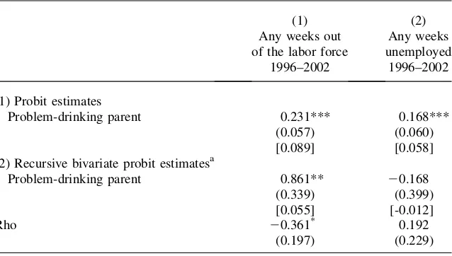
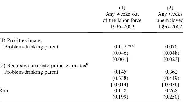
Results from this estimation are displayed in Tables 5 and 6. For men (Table 5), both probit and bivariate probit estimates show a positive and statistically significant effect of having a problem-drinking parent on the likelihood of being out of the labor force. The correlation term (rho) is different from zero at a statistical significance of 10 percent. Moreover, the sign of the bias is as expected; marginal effects are smaller in the bivariate probit estimation. A problem-drinking parent increases the likelihood that a son does not participate in the labor force by six percentage points in the bi-variate probit estimation, compared to nine percentage points in the probit model. In the case of unemployment, the probit coefficient for a problem-drinking parent is positive and statistically significant but neither rho nor the bivariate probit coefficient is statistically significant. For women (Table 6), there is a positive and statistically significant association between parental drinking and failure to participate in the la-bor force when using single equation regression, but no statistically significant effects of interest are found in the bivariate probit estimation.
V. Discussion and Conclusion
Using NLSY79, this paper studies the association between parental problem-drinking and children’s labor market outcomes at adulthood. Labor market outcomes are measured while the respondents are in their late 30s to mid-40s, a stage in which return to school or early retirement are less likely to be behind labor market decisions. Results from single equation regressions are suggestive of important inter-generation costs of problem-drinking. For men, having a problem-drinking parent is associated with longer periods out of the labor force, lengthier unemployment spells, and lower wages. For women, an association is identified between parental problem-drinking and time out of the labor force. While the analysis attempts to address endo-geneity, instrumental variables (GMM) estimation is not precise enough to conclude about the causality of these effects. On the other hand, results from bivariate probit estimation, a technique that addresses endogeneity but is less likely to be affected by low-powered instruments, support a negative effect of parental problem-drinking on male children’s labor force participation.
likely to start drinking by age 15 and more likely to be alcohol dependent ten and 15 years after the baseline interview. Most or all of these variables are endogenous and no causality can be inferred from the comparisons. However, we can at least speculate that the impacts on health conditions and alcohol use trajectories mediate some of the effects of problem-drinking parents on children’s labor force participa-tion and wages. Future research needs to address in more depth these links.
There are several limitations to the analysis. In the first place, around 5 percent of the sample that completed at least one of the 1996–2001 interviews did not respond to the questions about problem-drinking in the family. An initial mean comparison showed that these respondents belong to a fraction of the population with a higher risk of having alcoholic parents. The omission of these individuals from the final sample could be biasing our estimates toward zero.
A second problem may result from reporting bias. The data shows that the thresh-olds that males use to define an alcohol problem are different from those used by females. This may not be important if the extent to which an individual is affected by parental alcoholism depends on his or her personal or subjective threshold. In other words, an individual may have a lower threshold when defining ‘‘parental problem-drinking’’ because she or he is by nature more readily affected by such a problem. However, if thresholds are objective, male underreporting of parental problem-drinking will bias the results toward zero. Another type of reporting bias may result
Table 5
Effects of parental problem-drinking on the likelihood of being out of the labor force and of being unemployed (Male sample)
(1) Any weeks out of the labor force
1996–2002
(2) Any weeks unemployed
1996–2002
(1) Probit estimates
Problem-drinking parent 0.231*** 0.168***
(0.057) (0.060)
[0.089] [0.058]
(2) Recursive bivariate probit estimatesa
Problem-drinking parent 0.861** 20.168
(0.339) (0.399)
[0.055] [-0.012]
Rho 20.361* 0.192
(0.197) (0.229)
Note: Coefficients, standard errors in parentheses, and marginal effects in squared brackets. All estimations control for age, race, and state fixed effects for the respondent’s state of residency at age 14. *** Statisti-cally significant at 1 percent; ** StatistiStatisti-cally significant at 5 percent;*Statistically significant at 10 percent. a. Instruments used to identify reduced form problem-drinking equation are cigarette tax at state of birth, cigarette tax at mother’s state of birth in 1947 and problem-drinking grandfather. Chi2test of joint
signif-icance of instruments¼44.29 (p¼0.000)
from sicker people having a more distorted recall of their past family problems. Hav-ing objective quantitative information on parental drinkHav-ing would probably improve the consistency of the estimates and provide better information for policy purposes. At this point, I am unaware of any data set that can provide better information than the NLSY on parental drinking and on children’s long term labor market outcomes at a nationally representative level.
Third, it is possible that results are being led by problem-drinking fathers, conceal-ing other interestconceal-ing effects. Around 20 percent of respondents reported a problem-drinking father while only 4 percent admitted having a problem-problem-drinking mother. The small number of problem-drinking mothers in the data does not provide enough power to achieve statistically significant effects. If effects worked across gender lines (fathers affecting sons and mothers affecting daughters), as some literature and pre-liminary analyses of the data appeared to suggest, the weaker findings for females might be due to poor power rather than to genuine effects.
Fourth, the methodology in the main analysis relies on the use of an indicator of a problem-drinking grandfather as an instrumental variable. While the instrument sat-isfied formally the exclusion restrictions, its exogeneity could be questionable on the-oretical grounds. Thus, by using such variable, the expectation was to at least mitigate, but not necessarily eliminate biases due to endogeneity.
Table 6
Effects of parental problem-drinking on the likelihood of being out of the labor force and of being unemployed (Female sample)
(1) Any weeks out of the labor force
1996–2002
(2) Any weeks unemployed
1996–2002
(1) Probit estimates
Problem-drinking parent 0.157*** 0.070
(0.046) (0.048)
[0.061] [0.023]
(2) Recursive bivariate probit estimatesa
Problem-drinking parent 20.145 20.362
(0.338) (0.419)
[-0.014] [-0.036]
Rho 0.158 0.268
(0.199) (0.250)
Note: Coefficients, standard errors in parentheses, and marginal effects in squared brackets. All estimations control for age, race, and state fixed effects for the respondent’s state of residency at age 14. *** Statisti-cally significant at 1 percent; ** StatistiStatisti-cally significant at 5 percent;*Statistically significant at 10 percent. a. Instruments used to identify reduced form problem-drinking equation are beer tax at state of birth, whether there were alcohol controls at father’s state of birth in 1947 and problem-drinking grandfather. Chi2(3) test of joint significance of instruments¼61.21 (p¼0.000)
Table 7
Differences in Background Characteristics, Education, Health Status, Alcohol Use, and Labor Market Experience between Children of Problem-drinking Parentsaand Other Respondents
Male Respondents Female Respondents
Problem-drinking parent
No problem-drinking parent
Problem-drinking parent
No problem-drinking parent
Individual characteristics and family background (in 1979 or at age 14)
AFQT 39.583 40.101 38.072 38.550
Married in 1979 0.054 0.045 0.157 0.112***
Foreign language at age 14 0.210 0.232 0.224 0.232
Not religious 1979 0.158 0.116*** 0.106 0.076***
Attended religious services 1979 0.362 0.432*** 0.431 0.543***
Single parent family at age 14 0.232 0.166*** 0.223 0.162***
Stepparent family at age 14 0.159 0.061*** 0.142 0.060***
Other nonintact family structure at age 14 0.073 0.055*** 0.091 0.059***
Number of siblings 1979 3.955 3.822 4.055 3.839**
Ln average family income 1979/1980 10.456 10.591*** 10.307 10.506***
Ln poverty 1979 0.252 0.234 0.280 0.252**
Received public assistance 1979 0.181 0.132*** 0.199 0.143***
White collar father 0.219 0.245 0.207 0.254***
Adult female in household worked 0.549 0.516** 0.571 0.518***
Highest education family: no high school 0.338 0.322** 0.373 0.340**
Highest education family: high school 0.532 0.512** 0.514 0.498
Highest education in family: college or + 0.130 0.166** 0.113 0.161***
Balsa
Family had a library card (at age 14) 0.715 0.676** 0.722 0.719 Lived in same residence since birth (by 1979) 0.387 0.479*** 0.412 0.477***
Urban residency at age 14 0.840 0.784*** 0.811 0.792
County of residency crime rate in 1975 56.220 53.590** 54.680 54.278
County unemployment rate in 1979 6.420 6.235** 6.217 6.241
Education
No high school or GED 0.151 0.124** 0.113 0.089***
High school graduate 0.470 0.450 0.429 0.409
Some college 0.221 0.211 0.271 0.266
College graduate 0.108 0.119 0.105 0.132***
Graduate studies 0.051 0.095*** 0.082 0.103**
Highest grade completed 12.744 13.129*** 13.098 13.389***
Health
Depressive symptoms 1992 11.939 10.824*** 13.640 12.279***
Major depression 1992 0.127 0.093*** 0.176 0.143***
Any health limitations 1996–2002 0.176 0.126*** 0.235 0.183***
Alcohol use trajectory
Age started drinking 15.929 16.331*** 16.677 17.077***
Started drinking before age 15 0.321 0.250*** 0.196 0.139***
Alcohol dependent in 1989 or 1994 0.210 0.135*** 0.075 0.051***
Family characteristics 1996–2002
Married 1996–2002 0.411 0.480*** 0.449 0.493***
Separated 1996–2002 0.237 0.178*** 0.206 0.188
Labor market experience (by 1994)
Labor market experience (years) 12.015 12.458** 10.054 10.516***
Note: ** Difference between respondent with problem-drinking parent and respondent with no problem-drinking parent statistically significant at 5 percent; *** differ-ence statistically significant at 1 percent.
a. Parental problem-drinking¼1 when respondent reported either a biological or nonbiological problem-drinking mother or father.
478
The
Journal
of
Human
Fifth, the magnitudes of the standard errors in the GMM estimations raise con-cerns about the power of the instruments to identify statistically significant results. This imprecision limits our ability to say anything definitive about causality. Omitted variable bias could still be behind the detected associations between parental problem-drinking and children’s labor market outcomes.
The psychopathological consequences of parental drinking on adult children have received special attention in the area of psychology and family medicine. In econom-ics, however, none of the available estimates of the consequences of alcoholism used for policy purposes (to design, finance, and evaluate interventions) account for the impact of parental drinking on children. These estimates are restricted to measuring the direct health care costs, productivity losses, and crime costs imposed upon soci-ety by the individual with a drinking problem. This paper highlights the importance of accounting, in addition, for the losses in productivity suffered by adult sons of alcoholics, which are manifested through lower labor force participation and lower wages. Furthermore, it indicates the need to research and quantify the health care costs that children of alcoholics and society as a whole have to bare due to parental alcoholism. Policy recommendations, and in particular the types of interventions de-signed, may change substantially if these consequences are taken into consideration.
Appendix Table A1
Nonresponse and Attrition
Eligible, but not interviewed in 1996–2002
Interviewed at least once in 1996–2002
No response to parental alcohol
questions
Responded parental alcohol questions Final sample
Mean (1) (1) vs (3)a
Mean (2)
(2) vs (3)b Mean (3)
Standard
Deviation Minimum Maximum
N¼9,986 958 534 8,494
Labor market outcomes
Weeks out labor force (average 95, 97, 99, 01) N/A 10.814*** 8.650 14.908 0.000 52.000 Weeks unemployed (average 95, 97, 99, 01) N/A 1.786 1.843 5.002 0.000 52.000
Ln hourly wage (average 95, 97, 99, 01) N/A 2.591 2.602 0.720 0.009 5.687
Parental alcohol problems
Problem-drinking mother 0.044 N/A 0.043 0.2028 0.000 1.000
Problem-drinking father 0.161** N/A 0.204 0.4027 0.000 1.000
Demographics
Age 1979¼15 0.115 0.125 0.140 0.347 0.000 1.000
Age 1979¼16 0.148 0.125 0.138 0.345 0.000 1.000
Age 1979¼17 0.136 0.146 0.136 0.343 0.000 1.000
Age 1979¼18 0.113 0.154 0.139 0.346 0.000 1.000
Age 1979¼19 0.146 0.110 0.120 0.325 0.000 1.000
Age 1979¼20 0.136 0.127 0.106 0.307 0.000 1.000
Age 1979¼21 0.110 0.103 0.110 0.313 0.000 1.000
(continued)
480
The
Journal
of
Human
Appendix Table A1
(Continued)
Eligible, but not interviewed in 1996–2002
Interviewed at least once in 1996–2002
No response to parental alcohol
questions
Responded parental alcohol questions Final sample
Mean (1) (1) vs (3)a
Mean (2) (2) vs (3)b
Mean (3)
Standard
Deviation Minimum Maximum
Age 1979¼22 0.031 0.034 0.025 0.156 0.000 1.000
Whites 0.515 0.410*** 0.493 0.500 0.000 1.000
Hispanic 0.213** 0.292*** 0.188 0.391 0.000 1.000
Black 0.259*** 0.272** 0.307 0.461 0.000 1.000
Other race 0.013 0.026*** 0.011 0.106 0.000 1.000
Family background 1979 / age 14
AFQT 43.097*** 33.835*** 39.034 28.663 1.000 99.000
AFQT missing 0.180*** 0.172*** 0.040 0.197 0.000 1.000
Married in 1979 0.088 0.101 0.086 0.281 0.000 1.000
Foreign language 0.258** 0.346*** 0.228 0.419 0.000 1.000
Not religious 1979 0.122** 0.098 0.104 0.305 0.000 1.000
Catholic 0.354** 0.396*** 0.319 0.466 0.000 1.000
Baptist 0.199*** 0.201*** 0.274 0.446 0.000 1.000
Attended religious services 1979 0.435** 0.449 0.466 0.499 0.000 1.000
Single-parent family 0.184 0.205 0.177 0.382 0.000 1.000
Stepparent family 0.070 0.073 0.081 0.272 0.000 1.000
Other nonintact family structure 0.060 0.062 0.063 0.243 0.000 1.000
Balsa
Number of siblings 1979 3.759 3.972 3.875 2.672 0.000 22.000 Ln average family income 1979/1980 10.538 10.400** 10.507 1.092 0.000 12.914
Family income missing 0.086** 0.116*** 0.070 0.256 0.000 1.000
In poverty 1979 0.233 0.302*** 0.250 0.433 0.000 1.000
Poverty status missing 0.072** 0.075** 0.058 0.233 0.000 1.000
Received public assistance 1979 0.137 0.178** 0.150 0.357 0.000 1.000
Public assistance missing 0.030 0.054** 0.038 0.191 0.000 1.000
White collar father 0.269** 0.206** 0.239 0.426 0.000 1.000
White collar father missing 0.050 0.054 0.063 0.244 0.000 1.000
Adult female in household worked 0.477*** 0.494 0.530 0.499 0.000 1.000
Working status of female adult: missing 0.008 0.011 0.009 0.094 0.000 1.000 Highest education family: no high school 0.317 0.395*** 0.338 0.473 0.000 1.000 Highest education family: high school, no college 0.501 0.477 0.509 0.500 0.000 1.000 Highest education family: college or + 0.182*** 0.129 0.152 0.359 0.000 1.000
Family education missing 0.039 0.041 0.037 0.190 0.000 1.000
Family had a library card 0.729** 0.698 0.699 0.459 0.000 1.000
Residency 1979 or age 14
Lived in same residence since birth (by 1979) 0.436 0.412*** 0.461 0.499 0.000 1.000
Urban residency at age 14 0.799 0.825 0.795 0.404 0.000 1.000
County of residency crime rate in 1975 60.795*** 60.228*** 53.931 35.573 0.110 406.870
County crime rate missing 0.073* 0.094*** 0.057 0.232 0.000 1.000
County unemployment rate in 1979 6.303 6.418* 6.252 1.951 2.400 13.200
Unemployment rate missing 0.031 0.052*** 0.033 0.178 0.000 1.000
Region of residency 1979: North 0.246 0.218* 0.252 0.434 0.000 1.000
Region of residency 1979: South 0.294*** 0.332* 0.374 0.484 0.000 1.000
Region of residency 1979: West 0.205 0.216 0.189 0.392 0.000 1.000
Education
No high school or GED 0.161*** 0.169*** 0.111 0.314 0.000 1.000
High school graduate 0.366*** 0.423 0.437 0.496 0.000 1.000
(continued)
482
The
Journal
of
Human
Appendix Table A1
(Continued)
Eligible, but not interviewed in 1996–2002
Interviewed at least once in 1996–2002
No response to parental alcohol
questions
Responded parental alcohol questions Final sample
Mean (1) (1) vs (3)a
Mean (2) (2) vs (3)b
Mean (3)
Standard
Deviation Minimum Maximum
Some college 0.225 0.247 0.241 0.428 0.000 1.000
College graduate 0.155* 0.088 0.119 0.324 0.000 1.000
Graduate studies 0.093 0.073 0.092 0.289 0.000 1.000
Highest grade completed 13.107 12.768*** 13.182 2.494 0.000 20.000
Residency 1996–2002
Urban residency 1996–2002 N/A 0.756 0.748 0.358 0.000 1.000
Lived in the North 1996–2002 N/A 0.171*** 0.224 0.417 0.000 1.000
Lived in the South 1996–2002 N/A 0.371 0.389 0.488 0.000 1.000
Lived in the West 1996–2002 N/A 0.229*** 0.188 0.390 0.000 1.000
Changed regions 1996–2002 N/A 0.047 0.049 0.215 0.000 1.000
Region of residency missing 1996–2002 N/A 0.560*** 0.205 0.403 0.000 1.000
County of residency unemployment rate 1996–2002 N/A 6.410*** 6.087 2.307 2.040 18.125 Family characteristics 1996–2002
Married 1996–2002 N/A 0.468 0.474 0.499 0.000 1.000
Separated 1996–2002 N/A 0.139*** 0.191 0.393 0.000 1.000
Number of kids N/A 1.314 1.401 1.230 0.000 8.750
Balsa
Health
Depressive symptoms 11.640 12.012 11.851 8.395 0.000 56.000
Depressive symptoms missing 0.678*** 0.202*** 0.029 0.167 0.000 1.000
Major depression 0.140 0.150 0.125 0.331 0.000 1.000
Health limitations N/A 0.172 0.167 0.373 0.000 1.000
Health limitations missing N/A 0.011** 0.004 0.067 0.000 1.000
Alcohol use trajectory
Age started drinking 16.646 16.564 16.593 2.218 2.000 25.000
Started drinking before age 15 0.206 0.220 0.209 0.407 0.000 1.000
Alcohol dependent in 1989 or 1994 0.080** 0.059*** 0.104 0.305 0.000 1.000
Alcohol dependent missing 0.502 0.107*** 0.028 0.053 0.000 1.000
Labor market experience (by 1994)
Labor market experience (years) N/A 10.676 11.309 4.377 0.000 16.962
Labor market experience missing N/A 0.974*** 0.363 0.481 0.000 1.000
N 958 534 8,494
a. * Difference between mean (1) and mean (3) is statistically significant at 5 percent; *** difference statistically significant at 1 percent b. * Difference between mean (2) and mean (3) is statistically significant at 5 percent; *** difference statistically significant at 1 percent.
484
The
Journal
of
Human
References
Aizer, Anna. 2004. ‘‘Home Alone: Supervision after School and Child Behavior.’’Journal of Public Economics88(9–10):1835–48.
Amuedo-Dorantes, Catalina, and Traci Mach. 2002. ‘‘The Impact of Families on Juvenile Substance Use.’’Journal of Bioeconomics4(3):269–82.
Anda, Robert, Charles Whitfield, Vincent Felitti, Daniel Chapman, Valerie Edwards, Shanta Dube, and David Williamson. 2002. ‘‘Adverse Childhood Experiences, Alcoholic Parents, and Later Risk of Alcoholism and Depression.’’Psychiatric Services53(8):1001–09. Antecol, Heather, and Kelly Bedard. 2007. ‘‘Does Single Parenthood Increase the Probability
of Teenage Promiscuity, Substance Use and Crime?’’Journal of Population Economics 20(1):55–71.
Balsa, Ana. 2006. ‘‘The Impact of Parental Drinking on Children’s Utilization of Health Care Services.’’ Coral Gables: University of Miami. Unpublished.
Berger, Lawrence. 2005. ‘‘Income, Family Characteristics, and Physical Violence toward Children.’’Child Abuse and Neglect29(2):107–33.
The Book of States. 1947-64. Lexington, KY.: Council of the State Governments. Booth, Brenda, and Weiwei Feng. 2002. ‘‘The Impact of Drinking and Drinking
Consequences on Short-term Employment Outcomes in at-Risk Drinkers in Six Southern States.’’The Journal of Behavioral Health Services and Research29(2):157–66. Cameron, Lisa, and Jenny Williams. 2001. ‘‘Cannabis, Alcohol and Cigarettes: Substitutes or
Complements?’’Economic Record77(236):19–34
Chatterji, Pinka, and Sara Markowitz. 2001. ‘‘The Impact of Maternal Alcohol and Illicit Drug Use on Children’s Behavior Problems: Evidence from the Children of the National Longitudinal Survey of Youth.’’Journal of Health Economics20(5):703–31.
Chatterji, Pinka, and Jeff DeSimone. 2005. ‘‘Adolescent Drinking and High School Dropout.’’ NBER Working Paper No. W11337. Available at SSRN: http://ssrn.com/abstract¼723306 Connell, Arin, and Sherryl Goodman. 2002. ‘‘The Association between Psychopathology in Fathers Versus Mothers and Children’s Internalizing and Externalizing Behavior Problems: A Meta-Analysis.’’Psychological Bulletin128(5):746–73.
Dee, Thomas, and William Evans. 2003. ‘‘Teen Drinking and Educational Attainment: Evidence from Two-Sample Instrumental Variable Estimates.’’Journal of Labor Economics21(1):178–209.
Dobkin, Patricia, Richard Tremblay, Lyse Desmarais-Gervais, and Louise Depelteau. 1994. ‘‘Is Having an Alcoholic Father Hazardous for Children’s Physical Health?’’Addiction 89(12):1619–27.
Ellis, Deborah, Robert Zucker, and Hiram Fitzgerald. 1997. ‘‘The Role of Family Influences in Development and Risk.’’Alcohol Health and Research World21(3):218–26.
Feng, Weiwei, Wei Zhou, J.S. Butler, Brenda Booth, and Michael French. 2001. ‘‘The Impact of Problem-drinking on Employment,’’Health Economics10(6):509–21.
French, Michael, and Johanna Maclean. 2006. ‘‘Underage Alcohol Use, Delinquency, and Criminal Activity.’’Health Economics15(12):1261–81.
Garis, Dalton. 1998. ‘‘Poverty, Single-Parent Households, and Youth at-Risk Behavior: An Empirical Study.’’Journal of Economic Issues32(4):1079–06.
Hansen, Lars. 1982. ‘‘Large Sample Properties of Generalized Method of Moments Estimators.’’Econometrica50(3):1029–54.
Hayashi, Fumio. 2000.Econometrics.Princeton, N.J.: Princeton University Press. Jennison, Karen, and Kenneth Johnson. 1998. ‘‘Alcohol Dependence in Adult Children
of Alcoholics: Longitudinal Evidence of Early Risk.’’Journal of Drug Education28(1): 19–37.