07350015%2E2014%2E887013

(1)

Full Terms & Conditions of access and use can be found at

http://www.tandfonline.com/action/journalInformation?journalCode=ubes20

Download by: [Universitas Maritim Raja Ali Haji], [UNIVERSITAS MARITIM RAJA ALI HAJI

TANJUNGPINANG, KEPULAUAN RIAU] Date: 11 January 2016, At: 20:59

Journal of Business & Economic Statistics

ISSN: 0735-0015 (Print) 1537-2707 (Online) Journal homepage: http://www.tandfonline.com/loi/ubes20

A Nonparametric Test of the Predictive Regression

Model

Ted Juhl

To cite this article: Ted Juhl (2014) A Nonparametric Test of the Predictive Regression Model, Journal of Business & Economic Statistics, 32:3, 387-394, DOI: 10.1080/07350015.2014.887013 To link to this article: http://dx.doi.org/10.1080/07350015.2014.887013

Published online: 28 Jul 2014.

Submit your article to this journal

Article views: 227

View related articles

(2)

A Nonparametric Test of the Predictive

Regression Model

Ted JUHL

University of Kansas, 415 Snow Hall, Lawrence, KS 66045 (juhl@ku.edu)

This article considers testing the significance of a regressor with a near unit root in a predictive regression model. The procedures discussed in this article are nonparametric, so one can test the significance of a regressor without specifying a functional form. The results are used to test the null hypothesis that the entire function takes the value of zero. We show that the standardized test has a normal distribution regardless of whether there is a near unit root in the regressor. This is in contrast to tests based on linear regression for this model where tests have a nonstandard limiting distribution that depends on nuisance parameters. Our results have practical implications in testing the significance of a regressor since there is no need to conduct pretests for a unit root in the regressor and the same procedure can be used if the regressor has a unit root or not. A Monte Carlo experiment explores the performance of the test for various levels of persistence of the regressors and for various linear and nonlinear alternatives. The test has superior performance against certain nonlinear alternatives. An application of the test applied to stock returns shows how the test can improve inference about predictability.

KEY WORDS: Finance; Kernel regression; Near unit root; Time series.

1. INTRODUCTION

The predictive regression model has received much attention in recent years. In particular, the model where the regressors are persistent (with a unit root or near unit root) has been covered in the work of Campbell and Yogo (2006), Jansson and Moreira (2006), Lewellen (2004), and Stambaugh (1999), among others. The statistical estimation and testing of such models requires a treatment beyond the traditional normal approximations for the regression parameters. The persistence of the regressors directly affects the distribution of the standardt-ratio of the estimated regression parameters. The resulting distribution of the regres-sion parameter is related to the Dickey–Fuller distribution but with a nuisance parameter from the correlation of innovations to the unit root series in the future. The distribution is nonnormal so that standard asymptotic theory does not apply. Moreover, as the amount of correlation between innovations in the persistent series and the innovations in the regressand series increases, the distribution shifts to the right so that a type of “spurious” regression further distorts standard inference. These facts indi-cate the need for knowledge of the persistence of the regressor, or the need to develop new procedures that are “robust” to the unknown level of persistence in the regressor.

Given the above problems, Campbell and Yogo (2006), Jansson and Moreira (2006), and Lewellen (2004) each proposed solutions to inference when the level of persistence of the regressor is unknown and possibly contains a unit root (or near unit root). The approaches are related in that they attempt to find an optimal test in some class of statistics that are invariant to location and scale transformations of the data. The test we propose in this article shares the invariance properties of the above statistics. However, our test is designed to have power against linear and nonlinear alternatives. To accomplish this, we use nonparametric kernel estimation of the regression function. The estimated function is then tested to see if it is significantly different from a constant.

The nonparametric procedure that we use is based on two steps. First, we use nonparametric regression to estimate the relationship between the two series. The advantage of such an approach is that we are not required to posit a functional form for the relationship. One may have a theoretical basis for what the functional form may look like, but it could be that some unknown financial distortions may exist. By employing a non-parametric approach, we may detect an unforeseen relationship. For our purposes, we use kernel regression, and we employ a convenient reweighting procedure. Next, we see if the estimated regression function is correlated with the demeaned data. Such a procedure results in aU-statistic, and is known to be effec-tive in specification testing for stationary data. The novelty of using U-statistics for this problem is that we are able to test whether theentirefunction is a constant. Testing for the signif-icance of the function at a given number of points would then require some sort of Bonferroni argument which would become more conservative as we estimate more points of the function. By using theU-statistic approach, it is possible to test the null hypothesis that the entire function is a constant.

When testing the significance of regressors using nonpara-metric techniques, we have power against a much wider class of alternative hypotheses. Of course, with such generality comes a price in that power is not as high if there truly exists a linear relationship. We explore these costs via a Monte Carlo experi-ment. We find that the nonparametric test does outperform tests based on the linear for certain nonlinear alternatives.

The remainder of the article is organized as follows. In Sec-tion2, we describe the predictive regression model. Section3

provides an outline of the nonparametric test. The asymptotic results are derived in Section4and explored in a Monte Carlo

387

(3)

388 Journal of Business & Economic Statistics, July 2014

experiment detailed in Section5. An empirical illustration using stock returns is treated in Section6 and Section7concludes. Notation is standard with weak convergence denoted by→d . All limits in the article are taken as the sample sizeT _{→ ∞}.

2. PREDICTIVE REGRESSION MODEL

Let the variableyt denote the dependent variable in periodt

and letxt₋1denote a predictor variable observed at timet−1.

We are interested to see if there is any relationship betweenyt

andxt−1. We consider a model of the form

a “near” unit root. This is an extreme form of dependence in the predictor variable but one that serves as an approximation for the behavior of many financial ratios used in this type of analysis. Several studies have versions of this model where g(xt−1) is considered a linear function, and the findings suggest

that the distribution of OLS in the linear case is nonstandard and depends on the correlation betweenǫt andet. In light of

this result, Jansson and Moreira (2006), Campbell and Yogo (2006), Lewellen (2004), and others have proposed tests that are not based on the usualt-ratio of the OLS squares estimator of the slope coefficient forxt−1. The Jansson and Moreira (2006)

test is optimal in the class of conditionally unbiased tests, and the distribution of their test is also nonstandard, requiring a numerical integration routine to calculatep-values for the test for each new dataset.

In this article, we propose testing the predictive regression model using the nonparametric tests described in the next section.

3. NONPARAMETRIC TESTS FOR STATIONARY REGRESSORS

In this section, we summarize the type of nonparametric tests that we employ in this article. This type of test has been used when the data are assumed to be stationary as in Fan and Li (1996,1999) and Zheng (1996) among others. The idea is to check if two series are related without specifyinghowthey are related. That is, we allow for the series to have an unknown, perhaps nonlinear, relationship. To be specific, suppose thatyt

andxt−1are stationary series and that

yt =μy+g(xt−1)+ǫt, (3.1)

where E(ǫt|xt−1)=0 which implies that xt−1 andǫt are

un-correlated and that E(ǫt)=0. The model then implies that

E(ǫtg(xt−1))=0, which are the conditions used for nonlinear

least squares. The hypothesis that we wish to test is

H0:g(xt−1)=0

almost everywhere versus the alternative

H1:g(xt−1)=0

for some value ofxt₋1. Letp(xt₋1) be the density function of

xt₋1. To simplify the discussion in this section, suppose thatyt

has mean zero. Then using iterated expectations, we have

E[ytE(yt|xt−1)p(xt−1)]=E(E[ytE(yt|xt−1)p(xt−1)|xt−1])

g(xt−1)=0 almost everywhere. The above relation suggests

that we should find an estimate ofE[ytE(yt|xt−1)p(xt−1)] and

test whether the estimate is significantly different from zero. The nonparametric tests estimateE(yt|xt₋1)p(xt₋1) by kernel

regression ofyt onxt₋1 multiplied by the density estimate of

p(xt−1). That is,

whereK(·) is a kernel function andh is a bandwidth parame-ter.1The estimate ofE(yt|xt−1)p(xt−1) is particularly tractable

because the term ˆp(xt−1) cancels from the denominator,

elimi-nating the need for restricting the estimated density away from zero. This “reweighting” of the conditional mean was also em-ployed in Zheng (1996) and Fan and Li (1996). Moreover, we weight the estimated function by the estimated density to ac-count for the fact that even ifg(xt₋1) is nonzero, it may only

happen on a set with measure zero, hence the product of the function and the density will be zero. The final estimate of E(ytE(yt|xt−1)p(xt−1)) is the statistic

Inference is based on half of this quantity, which is given by

UT =

When the statistic UT is properly scaled, it is normally

dis-tributed under the null hypothesis thatg(xt−1)=0. Due to its

nonparametric construction, the test has power against a wide variety of alternatives, both linear and nonlinear.

4. DISTRIBUTION THEORY

The discussion in the last section is based on the assumption that the variables involved are stationary. Such results have been shown to hold when the independent variables satisfy some type of limit to the dependence, typically a condition stated in terms ofβ-mixing (absolute regularity), such as in Fan and Li (1999).

1_{For an introduction to kernel regression and nonparametric regression, see}

H¨ardle (1989a).

(4)

In this section, we provide the distribution theory when the independent variable is nonstationary in the form of a near unit root.

The model is

yt =μy+g(xt−1)+ǫt

xt =μx+ut

ut =ρTut−1+et.

The assumptions are listed below.

Assumption 1.

variance ofwtis 1, andǫthas finite fourth moments. The

char-acteristic function ofwtis given byϕ(t) such that|t|ϕ(t)→0

as|t_{| → ∞}.

Assumption 2. K(x) is nonnegative and bounded with

|x_|K(x)dx <_∞.

Assumption 3. T _{→ ∞}, h_→0, T h2_{→ ∞}, and T h4log2

T _→0.

These assumptions imply those used by Wang and Phillips (2012) for their cointegrated model.2_{Assumption 1 limits the} amount of dependence in the innovations of the process driving xt, so that the resultingU-statistic itself is a martingale which

is subject to the new central limit theorem. Assumption 2 is standard for kernels and Assumption 3 limits the rate at which the bandwidth goes to zero. Based on these assumptions, we can apply the model given in Wang and Phillips (2012) applies and gives the following result.

Theorem 4.1. Given Assumptions 1–3, under the null hy-pothesis thatg(xt−1)=0 almost everywhere, the statistic

T5/4√_h_U_ˆ

2_{In particular, the partial sums of (}_w

t, ǫt)⊤satisfy a multivariate invariance principal from Assumption 1. I thank an anonymous referee for suggesting a more lucid exposition.

It is important to note that the standardized version of the

U-statistic is exactly the same statistic analyzed in Fan and Li (1999), wherext is stationary with limited dependence (β

mix-ing). Because of this result, there is no need to change the statis-tical analysis of predictive regression models usingU-statistics if one is unsure about the possibility of a unit root in the variable xt−1. This fact is unusual in that standard OLS tests in

predic-tive regression models have a nonstandard limiting distribution ifxt−1 has a unit root or near unit root. Moreover, when using

OLS, the distribution depends on nuisance parameters such as the correlation betweenǫt andet. In our case, the limiting

dis-tribution does not change if the seriesxt−1is stationary or has a

unit root.

The result is different from existing results for nonparametric analysis of models with unit roots since all existing results are given by estimating the functionspointwise. One must have a method to test that the estimated function is constant almost ev-erywhere. As stated in the introduction, it is possible to construct a Bonferroni argument using pointwise results. However, as the number of estimated points increases, the confidence bands for the estimated function become more and more conservative. The advantage of theU-statistic approach is that we directly test the null hypothesis that the entire function is a constant.

From a practical point of view, the test is a good complement to the existing tests based on the linear model in that it may detect dependence inxt−1andyt that is nonlinear, and the tests

are not affected by assumptions about the dependence inxt−1.

One important consideration of nonparametric regression is the choice of bandwidth parameters. The assumptions used in Theorem 4.1 only require thathgoes to zero at some prescribed rate. No optimal bandwidth is proposed in this article, but we suggest usingh₌dσˆxT−1/5where dis a scalar and ˆσx is the

sample standard deviation ofxt−1. In our simulations, we try

various values ofd to gauge the sensitivity of the tests to the bandwidth parameter. One motivation for using a multiple of

ˆ

σx is that the statistic will become scale invariant. The test

is always location invariant but using a bandwidth that is a multiple of ˆσxensures scale invariance. Although this procedure

is similar to methods used in practice for stationary data, there is a difference when xt−1 is possibly integrated.3 The sample

standard deviation will diverge at rate√T asT _{→ ∞}, so that

hwill diverge at rateT3/10_{. An alternative is to use the sample}

standard deviation of xt−1, denoted ˆσx, which would be

appropriate ifxt−1contains a unit root, for example, and would

also remain scale invariant. In finite samples, it remains to be seen how the possible integration properties ofxt₋1 affect the

bandwidth, and, ultimately, the performance of theU-statistic. In the Monte Carlo section, we explore the performance of the

U-statistic using the sample standard deviation of both xt−1

andxt−1as a basis for the bandwidth.

5. MONTE CARLO EVIDENCE

We compare the nonparametric test with the two leading tests developed by Campbell and Yogo (2006) and Jansson and

3_{We thank an anonymous referee for pointing out the divergence and the}

poten-tial problem with the resulting bandwidth.

(5)

Moreira (2006). The experiment uses the following model:

yt =μy+g(xt₋1)+ǫt

xt =ρTxt₋1+et.

We set the parameterσǫe= −0.75 and−0.95, values that are

consistent with the empirical regularities found in financial data. For example, if xt−1 represents a dividend–price ratio

and yt represents a stock return, then a positive shock to

returns in the form of a large value of ǫt would then cause

a concurrent decrease in the dividend–price ratio, so that the correlation between et and ǫt should be negative. Lewellen

(2004) estimated values ofσǫe ranging from −0.88 to −0.96

for various financial ratios used forxt−1.

We consider several possible levels of persistence in xt

through the parameterρ. In particular, we parameterizeρas

ρT =1−

c T

so thatρTis “local to unity.” The values ofcused in the

simula-tion are 0, 5, 10, 15, and 20. In this first experiment, we examine the size properties of the test. That is, we generate the data so thatg(xt−1)=0 and we tabulate the percentage of rejections in

10,000 replications. The sample sizes considered areT ₌100, T ₌500, andT ₌1000. There are four different bandwidth parameters that are examined for theUT statistic. The statistics

denoted by U1 and U2 use h₌σˆxT−1/5 andh=2 ˆσxT−1/5,

respectively. The statistics Ud1 and Ud2 use bandwidth param-eters that are based on the standard deviation of the differences ofxt, so that the respective bandwidth parameters are given by

h₌σˆxT−1/5andh=2 ˆσxT−1/5The statistic of Jansson and

Moreira (2006) is a uniformly most powerful conditionally un-biased test in the linear model, so it is denoted and UMPCU. The Campbell and Yogo test uses a Bonferroni bound and we denote this test as CYB. For comparison purposes, we include an OLS

t-test that the linear regression coefficient on xt−1 is zero and

denote this as TSTAT. This test is incorrect in the case whenxt

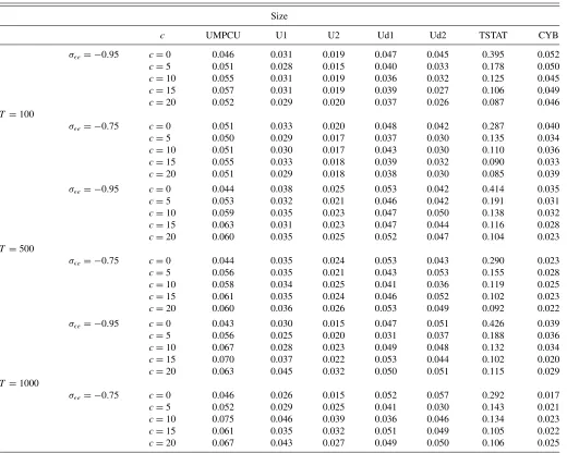
has a unit root or root local to unity, but is included to illustrate the potential problems of ignoring the extreme dependence in xt₋1. The sizes of the tests appear inTable 1.

FromTable 1, we see that the UMPCU and CYB tests have size close to the nominal size in all cases. The U-statistic is conservative and gets more conservative for a larger bandwidth. As discussed earlier, thet-statistic is not normally distributed and we included this statistic to show the costs of ignoring the

Table 1. Size of competing tests

Size

c UMPCU U1 U2 Ud1 Ud2 TSTAT CYB

σǫe = −0.95 c=0 0.046 0.031 0.019 0.047 0.045 0.395 0.052

c=5 0.051 0.028 0.015 0.040 0.033 0.178 0.050

c=10 0.055 0.031 0.019 0.036 0.032 0.125 0.045

c₌15 0.057 0.031 0.019 0.039 0.027 0.106 0.049

c=20 0.052 0.029 0.020 0.037 0.026 0.087 0.046

T =100

σǫe = −0.75 c=0 0.051 0.033 0.020 0.048 0.042 0.287 0.040

c=5 0.050 0.029 0.017 0.037 0.030 0.135 0.034

c=10 0.051 0.030 0.017 0.043 0.030 0.110 0.036

c=15 0.055 0.033 0.018 0.039 0.032 0.090 0.033

c₌20 0.051 0.029 0.018 0.038 0.030 0.085 0.039

σǫe = −0.95 c=0 0.044 0.038 0.025 0.053 0.042 0.414 0.035

c=5 0.053 0.032 0.021 0.046 0.042 0.191 0.031

c=10 0.059 0.035 0.023 0.047 0.050 0.138 0.032

c=15 0.063 0.031 0.023 0.047 0.044 0.116 0.028

c=20 0.060 0.035 0.025 0.052 0.047 0.104 0.023

T =500

σǫe = −0.75 c=0 0.044 0.035 0.024 0.053 0.043 0.290 0.023

c₌5 0.056 0.035 0.021 0.043 0.053 0.155 0.028

c=10 0.058 0.034 0.025 0.041 0.036 0.119 0.025

c₌15 0.061 0.035 0.024 0.046 0.052 0.102 0.023

c=20 0.060 0.036 0.026 0.053 0.049 0.092 0.022

σǫe = −0.95 c=0 0.043 0.030 0.015 0.047 0.051 0.426 0.039

c=5 0.056 0.025 0.020 0.031 0.037 0.188 0.036

c=10 0.067 0.028 0.023 0.049 0.048 0.132 0.034

c=15 0.070 0.037 0.022 0.053 0.044 0.102 0.020

c₌20 0.063 0.045 0.032 0.050 0.051 0.115 0.029

T =1000

σǫe = −0.75 c=0 0.046 0.026 0.015 0.052 0.057 0.292 0.017

c=5 0.052 0.029 0.025 0.041 0.030 0.143 0.021

c=10 0.075 0.046 0.039 0.036 0.046 0.134 0.023

c=15 0.061 0.035 0.032 0.051 0.049 0.105 0.022

c=20 0.067 0.043 0.027 0.049 0.050 0.106 0.025

(6)

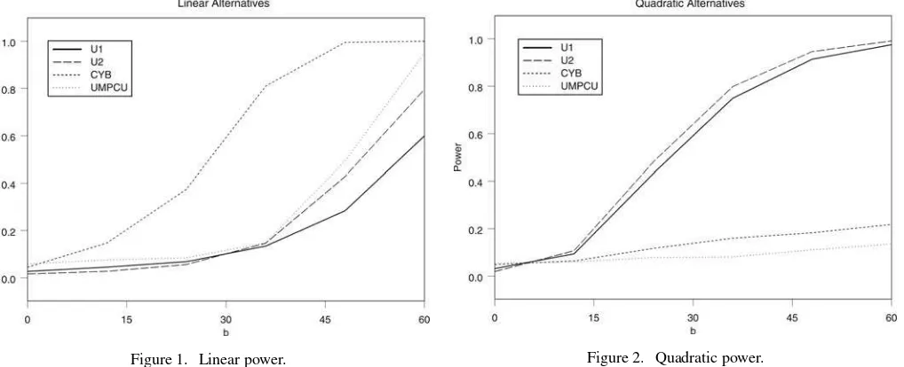
Figure 1. Linear power.

unit root behavior ofxt−1. At a nominal size of 5%, we reject the

null hypothesis of no predictability approximately 40% of the time when the innovations from the regressors and regressand are highly correlated. When the parameter c increases (near unit root), the normal approximation becomes less damaging. However, even when c₌5 with an autoregressive parameter ofρT =0.95, we reject the null roughly 18% of the time. The

sample sizeTappears to have a minor affect on the performance of all the tests considered in the experiment. In general, the bandwidth associated with the standard deviation ofxt−1 (U1

and U2) are more conservative than those associated with the standard deviation ofxt−1(Ud1 and Ud2).

To determine the sensitivity of the U-statistic to possible asymmetric distributions, we generate the same data using a centered χ2

1 distribution which is clearly skewed. The

experiment produces results that are very similar to those inTable 1, and suggest that the normal distribution is still a reasonable approximation for the test statistic even if the errors are not from a symmetric distribution.4

For power comparisons, we now consider three alternative functions. In the first case, the alternative is linear so that

g(xt−1)=βxt−1.

For purposes of comparison with Jansson and Moreira (2006), we setβ₌ 1−σ2

eǫγ, withγ =b/T, and letbincrease. The

power functions for linear alternatives are shown inFigure 1.5 We notice that the Bonferroni test procedure of Campbell and Yogo (2006) dominates all other tests for linear alternatives. Even though our U-statistics are less powerful than the tests based on linear alternatives, they still have power against linear alternatives

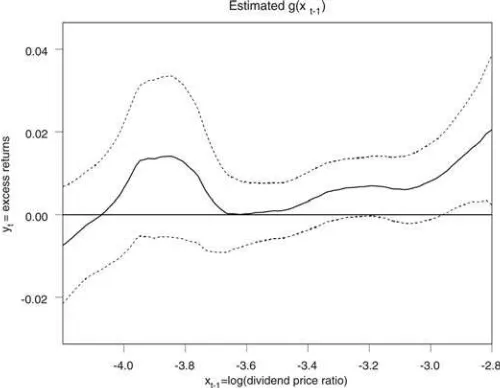
For an example of a nonlinear alternative, we let

g(xt−1)=βxt2−1,

so that the alternative is a quadratic. The quadratic is included as an example of a nonmonotonic function where linearity would have little power. Moreover, in the empirical section,

4_{The results are available upon request.}

5_{We use}_T

=100 for all of the power figures.

Figure 2. Quadratic power.

the relationship involving 3-month Treasury bill rates exhibits a similar shape over the middle region of historical rates. The power curves are presented inFigure 2. As expected, the

U-statistics have the highest power. One phenomenon that we found for quadratic alternatives was that the linear based tests (UMPCU and CYB) had power functions that reached a plateau at around 30% and never increased. This power function shows the possible gains from using a U-statistic in predictive regression models.

For a different alternative, we consider a nonlinear function that is monotonic. The quadratic alternative gives a distinct advantage to theU-statistic approach since a linear regression estimate will be near zero. If we choose an alternative that remains monotonic, such an advantage may disappear so that the tests based on linear alternatives will again have higher power. Our alternative is given by

g(xt−1)=βxt3−1.

The power curve is shown in Figure 3. The power of the U

statistic is less than the competing tests since for this cubic alternative, the relationship is monotonic.

Figure 3. Cubic power.

(7)

The final alternative is a step function that depends on a “threshold” value. In particular, the function is given by

g(xt−1)=β1(xt−1 >0)

so that the threshold is zero. From the figure, the power for theU

statistics is much higher than the tests based on linear models, and we see the value of considering nonlinear alternatives in predictive regressions. The tests based on linear models have power less than size and power decreases as the size of the step increases.

6. EMPIRICAL APPLICATIONS

The procedures discussed in this article can be used to test the significance of the regressorxt₋1without specifying a functional

form. We use a subset of the data discussed in Campbell and Yogo (2006) and a full description of the data and sources can be found there. We letytrepresent excess monthly returns from

the NYSE/AMEX value-weighted index from 1952 to 2002. Moreover, the excess returns are calculated by subtracting the one-month T-bill rate for each month. The seriesxt represents

four different series taken in turn; the log of the dividend–price ratio computed using dividends over the past year divided by price, the log of earnings price ratio, the 3-month T-bill rate, and the long–short yield spread.6_{We have 612 observations. The unit} root test of Elliott, Rothenberg, and Stock (1996) is calculated using the modified SIC and Akaike criteria developed in Ng and Perron (2001) to select the number of lags in the test. One lag of xt is selected by both criteria and the test value is−0.243

which is not significant at the 10% level. Hence, we fail to reject the unit root hypothesis for the log of the dividend-price ratio. This suggests that a standardt-ratio in a regression ofyt

onxt−1would not be well approximated by a standard normal

distribution.7 In light of the persistence in xt−1, we employ

the procedure in Campbell and Yogo (2006) using theQ-test. Based on inverting theQ-test, a 90% confidence interval for the regression parameter is (−0.004,0.010) which contains zero. Hence, there is no evidence forlinearpredictability of returns using the log of the dividend–price ratio.

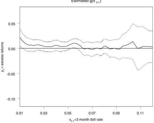
To consider the possibility of a nonlinear relationship, we conduct a nonparametric kernel regression of yt on xt−1. As

noted in Bandi (2004), kernel regression can be standardized so that the normal approximation still holds ifxt−1has a unit root

or near unit root. We tried several bandwidth parameters, and the results were not sensitive within a large range of bandwidths. A representative graph of the estimated function as well as 95% pointwise confidence bands is shown inFigure 5using a bandwidth ofh₌σxT−1/5.

There are several features to note about the estimated regres-sion function inFigure 5. Although the estimated function looks highly nonlinear, we notice that the 95% pointwise confidence bands contain zero when the log dividend–price ratio is low, so that the null hypothesis of no effect cannot be rejected.

6_{The long yield is the Moody’s seasoned Aaa corporate bond yield.}

7_From_{Table 1}_{, we see that if the null hypothesis of no relationship between}_y t andxt−1is true, we would still reject the null hypothesis around 40% of the time.

Figure 4. Threshold power.

However, at higher levels of the log dividend–price ratio, zero is not in the confidence bands, and so one would presume that we can reject the null of no effect ofxt−1onyt for higher levels of

xt−1. However, this is not a valid statistical argument. The width

of each confidence interval is based on a pointwise argument which means at each point, the confidence interval is valid if we consider the functionat that point in isolation. However, in this graph, we have estimated the function at 612 points. Therefore, the confidence bands shown in the graph are not confidence bands for the entire function. One adjustment is to use a Bonferroni argument to make the confidence bands wider. Such an adjustment is often extremely conservative, especially when many points of the function are estimated, as in this case. Eubank and Speckman (1993) compared the pointwise bands with the conservative Bonferroni bands to verify the increased width. An alternative approach is to construct asymptotically accurate confidence bands using the approach of H¨ardle (1989b). Such an approach involves constructing confidence bands based on the maximal deviation of the Gaussian process

Figure 5. Dividend price ratio function.

(8)

Figure 6. Earnings price ratio function.

associated with the kernel estimator over the range of the data. Moreover, it is unknown if such an approach is valid when the data have any type of dependence.

An alternative to correcting the confidence bands for the non-parametric regression function is to simply construct the U -statistic developed in this article. We calculate the test and get a value of 0.33. TheU-statistic is normally distributed and rejects for large values. Hence, we fail to reject the null hypothesis of no predictability (g(xt−1)=0). In fact, the p-value for a test

statistic of 0.33 is 0.38, so that there is very little evidence of predictability. Inference using theU-statistic changes the con-clusion found using a nonparametric function with pointwise confidence bands.

Next, consider the relationship between excess returns and the log of the earnings price ratio, one of the variables considered in the forecasting model of Lettau and Ludvigson (2001). As noted in Campbell and Yogo (2006), the unit root hypothesis is not rejected for this data series. We plot estimated nonparametric

Figure 7. T-bill function.

Figure 8. Yield spread function.

function and along with the 95% pointwise confidence bands inFigure 6. Even using the pointwise confidence bands, there appears to be no evidence of predictability. TheU-statistic takes a value of −0.28 with ap-value of 0.61, which confirms the graphical evidence for lack of predictability.

The relationship between excess returns and 3-month Trea-sury bill rates is explored in Figure 7. Again, there is little evidence of predictability, and theU-statistic of−0.54 with a

p-value of 0.71 confirms.

Finally, as in Boudoukh, Richardson, and Whitelaw (1997), the predictive regression is estimated using the yield spread as a predictor. The 95% confidence interval for the largest root of the series does not contain one, but Campbell and Yogo (2006) noted that the upper limit is 0.968. We plot the estimated relationship between excess returns and the yield spread in Figure 8. The estimated function and pointwise confidence bands suggest pre-dictability that is significantly different from zero in the middle range of the spread values. The function is nonmonotonic with the predictability disappearing is either tail of the distribution of the spread. TheU-statistic takes a value of 2.19 with ap-value of 0.02, so that we reject the null hypothesis of no predictability. The use of theU-statistic shows that the predictability is not just an artifact of the pointwise confidence bands being too narrow.8

7. CONCLUSION

In this article, we have examined nonparametric tests applied to predictive regression models. In particular, we have applied recent results of Wang and Phillips (2012) for cointegrated mod-els to tests based onU-statistics for the predictive regression model. The most useful feature of the tests is the lack of the so-called razor’s edge in asymptotic theory typically associated with unit root models. The limiting distribution for the properly

8_{I also test the null of linearity using the}_U_{-statistic proposed in Zheng (}₁₉₉₆_).

The test is based on residuals from a linear model and uses the same bandwidth as the nonparametric tests proposed in this article. The variable used is the yield spread and find ap-value of 0.0985, so that there is some evidence that the relationship is nonlinear.

(9)

standardized statistic is standard normal if the predictor variable is stationary or if it has a unit root.

A Monte Carlo experiment shows that the test has good size properties and has power against some nonlinear alternatives that tests based on linear models tend to miss. In particular, if the alternative is nonmonotonic, theU-statistic based tests have a distinct advantage.

An empirical section is used to show the usefulness of the test. In one example, we fail to find evidence for predictabil-ity of returns using the log dividend–price ratio as a predictor. The example shows how the test is an important complement to tests based on a linear model and standard nonparametric estimation. In particular, the nonparametricU-statistic provides a way to circumvent the currently intractable problem of find-ing accurate (not conservative) uniform confidence bands for nonparametric regression functions if the regressor has a unit root. In our example, pointwise confidence bands suggest the existence of predictability of returns at very high levels of the dividend–price ratio. However, this is due to the liberal nature of pointwise confidence bands. In the example using the yield spread, we find some evidence of predictability where the sig-nificance of the predictability is apparent only in the middle range of the data. Moreover, there is evidence that we can re-ject a linear model for this data. These applications serve to illustrate that the proposed U-statistic provides a simple way to test the significance of a nonparametric regression function uniformly across all observed data in a predictive regression model.

ACKNOWLEDGMENTS

We thank an Associate Editor, two anonymous referees, Roger Koenker, Peter Phillips, Zhongjun Qu, and Zhijie Xiao for comments on earlier versions of this article. I thank Michael Jansson for providing the code for his procedures.

[Received May 2013. Revised November 2013.]

REFERENCES

Bandi, F. M. (2004), “On the Persistence and Nonparametric Estima-tion With an ApplicaEstima-tion to Stock Return Predictability,” Graduate School of Business, University of Chicago, available at http://faculty. chicagobooth.edu/federico.bandi/research/b04.pdf. [392]

Boudoukh, J., Richardson, M., and Whitelaw, R. F. (1997), “Nonlinearities in the Relation Between the Equity Premium and the Term Structure,”

Management Science, 43, 371–385. [393]

Campbell, J. Y., and Yogo, M. (2006), “Efficient Tests of Stock Re-turn Predictability,” Journal of Financial Economics, 81, 27–60. [387,388,389,391,392,393]

Elliott, G., Rothenberg, T. J., and Stock, J. H. (1996), “Efficient Tests for an Autoregressive Unit Root,”Econometrica, 64, 813–836. [392]

Eubank, R., and Speckman, P. (1993), “Confidence Bands in Nonparametric Regression,”Journal of the American Statistical Association, 88, 1287– 1300. [392]

Fan, Y., and Li, Q. (1996), “Consistent Model Specification Tests: Omitted Variables and Semi-Parametric Functional Forms,”Econometrica, 64, 865– 890. [388]

——— (1999), “Central Limit Theorem for Degenerate U-Statistics of Abso-lutely Regular Processes With Applications to Model Specification Testing,”

Journal of Nonparametric Statistics, 10, 245–271. [388,389]

H¨ardle, W. (1989a),Applied Nonparametric Regression, Cambridge: Cambridge University Press. [388]

——— (1989b), “Asymptotic Maximal Deviation of M-Smoothers,”Journal of Multivariate Analysis, 29, 163–179. [392]

Jansson, M., and Moreira, M. J. (2006), “Optimal Inference in Regression Models With Nearly Integrated Regressors,”Econometrica, 74, 681–714. [387,388,390,391]

Lettau, M., and Ludvigson, S. (2001), “Consumption, Aggregate Wealth, and Expected Stock Returns,”Journal of Finance, 56, 815–849. [393] Lewellen, J. (2004), “Predicting Returns with Financial Ratios,”Journal of

Financial Economics, 74, 209–235. [387,388,390]

Ng, S., and Perron, P. (2001), “Lag Length Selection and the Construction of Unit Root Tests With Good Size and Power,”Econometrica, 69, 1519–1554. [392]

Stambaugh, R. F. (1999), “Predictive Regressions,”Journal of Financial Eco-nomics, 54, 375–421. [387]

Wang, Q., and Phillips, P. C. B. (2012), “A Specification Test for Nonlinear Nonstationary Models,”The Annals of Statistics, 40, 727–758. [389,393] Zheng, J. X. (1996), “A Consistent Test of Functional Form via Nonparametric

Estimation Techniques,”Journal of Econometrics, 75, 263–290. [388,393]