Full Terms & Conditions of access and use can be found at
http://www.tandfonline.com/action/journalInformation?journalCode=ubes20
Download by: [Universitas Maritim Raja Ali Haji] Date: 11 January 2016, At: 22:25
Journal of Business & Economic Statistics
ISSN: 0735-0015 (Print) 1537-2707 (Online) Journal homepage: http://www.tandfonline.com/loi/ubes20
Forecast Rationality Tests Based on Multi-Horizon
Bounds
Andrew J. Patton & Allan Timmermann
To cite this article: Andrew J. Patton & Allan Timmermann (2012) Forecast Rationality Tests Based on Multi-Horizon Bounds, Journal of Business & Economic Statistics, 30:1, 1-17, DOI: 10.1080/07350015.2012.634337
To link to this article: http://dx.doi.org/10.1080/07350015.2012.634337
Published online: 22 Feb 2012.
Submit your article to this journal
Article views: 1229
View related articles
January 8, 2011.
Forecast Rationality Tests Based on
Multi-Horizon Bounds
Andrew J. P
ATTONDepartment of Economics, Duke University, 213 Social Sciences Building, Box 90097, Durham, NC 27708 ([email protected])
Allan TIMMERMANN
University of California, San Diego, 9500 Gilman Dr., La Jolla, CA 92093 ([email protected])
Forecast rationality under squared error loss implies various bounds on second moments of the data across forecast horizons. For example, the mean squared forecast error should be increasing in the horizon, and the mean squared forecast should be decreasing in the horizon. We propose rationality tests based on these restrictions, including new ones that can be conducted without data on the target variable, and implement them via tests of inequality constraints in a regression framework. A new test of optimal forecast revision based on a regression of the target variable on the long-horizon forecast and the sequence of interim forecast revisions is also proposed. The size and power of the new tests are compared with those of extant tests through Monte Carlo simulations. An empirical application to the Federal Reserve’s Greenbook forecasts is presented.
KEY WORDS: Forecast optimality; Forecast horizon; Real-time data; Survey forecasts.
1. INTRODUCTION
Forecasts recorded at multiple horizons, for example, from one to several quarters into the future, are commonly reported in empirical work. For example, the surveys conducted by the Philadelphia Federal Reserve (Survey of Professional Forecast-ers), Consensus Economics or Blue Chip and the forecasts pro-duced by the IMF (World Economic Outlook), the Congres-sional Budget office, the Bank of England and the Board of the Federal Reserve all cover multiple horizons. Similarly, econo-metric models are commonly used to generate multi-horizon forecasts, see, for example, Clements (1997), Faust and Wright (2009), and Marcellino, Stock and Watson (2006). The avail-ability of such multi-horizon forecasts provides an opportunity to devise tests of optimality that exploit the information in the complete “term structure” of forecasts recorded across all hori-zons. By simultaneously exploiting information across several horizons, rather than focusing separately on individual horizons, multi-horizon forecast tests offer the potential of drawing more powerful conclusions about the ability of forecasters to produce optimal forecasts. This article derives a number of novel and simple implications of forecast rationality and compares tests based on these implications with extant methods.
A well-known implication of forecast rationality is that, un-der squared-error loss, the mean squared forecast error should be a weakly increasing function of the forecast horizon, see, for example, Diebold (2001), and Patton and Timmermann (2007a). A similar property holds for the forecasts themselves: Internal consistency of a sequence of optimal forecasts implies that the variance of the forecasts should be a weakly decreasing function of the forecast horizon. Intuitively, this property holds because the variance of the expectation conditional on a large informa-tion set (corresponding to a short forecast horizon) must exceed
that of the expectation conditional on a smaller information set (corresponding to a long horizon). It is also possible to show that optimal updating of forecasts implies that the variance of the forecast revision should exceed twice the covariance between the forecast revision and the actual value. It is uncommon to test such variance bounds in empirical practice, in part due to the difficulty in setting up joint tests of these bounds. We suggest and illustrate testing these monotonicity properties via tests of inequality constraints using the methods of Gourieroux, Holly, and Monfort (1982) and Wolak (1987,1989), and the bootstrap methods of White (2000) and Hansen (2005).
Tests of forecast optimality have conventionally been based on comparing predicted and realized values of the outcome vari-able. This severely constrains inference in some cases since, as shown by Croushore (2006), Croushore and Stark (2001), and Corradi, Fernandez, and Swanson (2009), revisions to macroe-conomic variables can be very considerable and so raises ques-tions that can be difficult to address such as “What are the forecasters trying to predict?”, that is first-release data or final revisions. We show that variations on both the new and extant optimality tests can be applied without the need for observa-tions on the target variable. These tests are particularly useful in situations where the target variable is not observed (such as for certain types of volatility forecasts) or is measured with considerable noise (as in the case of output forecasts).
Conventional tests of forecast optimality regress the realized value of the predicted variable on an intercept and the fore-cast for a single horizon and test the joint implication that the
© 2012American Statistical Association Journal of Business & Economic Statistics
January 2012, Vol. 30, No. 1 DOI:10.1080/07350015.2012.634337
1
intercept and slope coefficient are 0 and 1, respectively (Mincer and Zarnowitz1969). In the presence of forecasts covering mul-tiple horizons, a complete test that imposes internal consistency restrictions on the forecast revisions is shown to give rise to a univariate optimal revision regression. Using a single equa-tion, this test is undertaken by regressing the realized value on an intercept, the long-horizon forecast and the sequence of intermediate forecast revisions. A set of zero–one equality restrictions on the intercept and slope coefficients are then tested. A key difference from the conventional Mincer–Zarnowitz test is that the joint consistency of all forecasts at different horizons is tested by this generalized regression. This can substantially increase the power of the test.
Analysis of forecast optimality is usually predicated on co-variance stationarity assumptions. However, we show that the conventional assumption that the target variable and forecast are (jointly) covariance stationary is not needed for some of our tests and can be relaxed provided that forecasts for different horizons are lined up in “event time,” as studied by Nordhaus (1987), Davies and Lahiri (1995), Clements (1997), Isiklar, Lahiri, and Loungani (2006), and Patton and Timmermann (2010b,2011). In particular, we show that the second moment bounds continue to hold in the presence of structural breaks in the variance of the innovation to the predicted variable and other forms of data heterogeneity.
To shed light on the statistical properties of the variance bound and regression-based tests of forecast optimality, we undertake a set of Monte Carlo simulations. These simulations consider various scenarios with zero, low, and high measurement error in the predicted variable and deviations from forecast optimal-ity in different directions. We find that the covariance bound and the univariate optimal revision test have good power and size properties. Specifically, they are generally better than con-ventional Mincer–Zarnowitz tests conducted for individual hori-zons, which either tend to be conservative, if a Bonferroni bound is used to summarize the evidence across multiple horizons, or suffer from substantial size distortions, if the multi-horizon re-gressions are estimated as a system. Our simulations suggest that the various bounds and regression tests have complemen-tary properties in the sense that they have power in different directions and so can identify different types of suboptimal be-havior among forecasters.
An empirical application to the Federal Reserve’s Greenbook forecasts of GDP growth, changes to the GDP deflator, and con-sumer price inflation confirms the findings from the simulations. In particular, we find that conventional regression tests often fail to reject the null of forecast optimality. In contrast, the new vari-ance bound tests and single-equation multi-horizon tests have better power and are able to identify deviations from forecast optimality.
The outline of the article is as follows. Section 2 presents some novel variance bound implications of optimality of fore-casts across multiple horizons and the associated tests. Section 3 considers regression-based tests of forecast optimality and Sec-tion 4 presents some extensions of our main results to cover data heterogeneity and heterogeneity in the forecast horizons. Sec-tion 5 presents results from a Monte Carlo study, while SecSec-tion 6 provides an empirical application to Federal Reserve Greenbook forecasts. Section 7 concludes this article.
2. MULTI-HORIZON BOUNDS AND TESTS
In this section, we derive variance and covariance bounds that can be used to test the optimality of a sequence of forecasts recorded at different horizons. These are presented as corollar-ies to the well-known theorem that the optimal forecast under quadratic loss is the conditional mean. The proofs of these corol-laries are collected in the Appendix.
2.1 Assumptions and Background
Consider a univariate time series,Y ≡ {Yt;t=1,2, . . .}, and
suppose that forecasts of this variable are recorded at dif-ferent points in time,t =1, . . . , T and at different horizons, h=h1, . . . , hH. Forecasts ofYtmadehperiods previously will
be denoted as ˆYt|t−h,and are assumed to be conditioned on the
information set available at timet−h,Ft−h, which is taken
to be the filtration ofσ-algebras generated by{Z˜t−h−k;k≥0},
where ˜Zt−h is a vector of predictor variables. This need not
(only) comprise past and current values ofY. Forecast errors are given byet|t−h=Yt−Yˆt|t−h.We consider an (H×1) vector
of multi-horizon forecasts for horizons h1< h2 <· · ·< hH,
with generic long and short horizons denoted by hL and hS
(hL> hS).Note that the forecast horizons,hi,can be positive,
zero, or negative, corresponding to forecasting, nowcasting, or backcasting, and further note that we do not require the forecast horizons to be equally spaced.
We will develop a variety of forecast optimality tests based on corollaries to Theorem 1 discussed later. In so doing, we take the forecasts as primitive, and if the forecasts are generated by particular econometric models, rather than by a combina-tion of modeling and judgemental informacombina-tion, the estimacombina-tion error embedded in those models is ignored. In the presence of estimation error, the results established here need not hold in finite samples (Schmidt1974; Clements and Hendry1998). Existing analytical results are very limited, however, as they as-sume a particular model (e.g., an AR(1) specification) and use inadmissible forecasts based on plug-in estimators. In practice, forecasts from surveys and forecasts reported by central banks reflect considerable judgmental information, which is difficult to handle using the methods developed by West (1996) and West and McCracken (1998).
The “real time” macroeconomics literature has demonstrated the presence of large and prevalent measurement errors affecting a variety of macroeconomic variables, see Corradi, Fernandez, and Swanson (2009), Croushore (2006), Croushore and Stark (2001), Diebold and Rudebusch (1991), and Faust, Rogers, and Wright (2005). In such situations, it is useful to have tests that do not require data on the target variable and we present such tests below. These tests exploit the fact that, under the null of forecast optimality, the short-horizon forecast can be taken as a proxy for the target variable, from the standpoint of longer horizon forecasts, in the sense that the inequality results pre-sented earlier all hold when the short-horizon forecast is used in place of the target variable. Importantly, unlike standard cases, the proxy in this case issmootherrather than noisier than the actual variable. This has beneficial implications for the finite sample performance of these tests when the measurement error is sizeable or the predictiveR2of the forecasting model is low.
Under squared-error loss, we have the following well-known theorem (see, e.g., Granger1969):
Theorem 1 (Optimal Forecast Under MSE Loss). Assume that the forecaster’s loss function is quadratic,L(y,yˆ)=(y−
ˆ
y)2, and that the conditional mean of the target variable given
the filtrationFt−h,E[Yt|Ft−h],is a.s. finite for allt. Then
ˆ
Yt∗|t−h≡arg min
ˆ y∈Y
E[(Yt−yˆ)2|Ft−h]=E[Yt|Ft−h], (1)
whereY⊆Ris the set of possible values for the forecast.
Some of the results derived below will make use of a standard covariance stationarity assumption:
Assumption S1: The target variable, Yt, is generated by a
covariance stationary process.
2.2 Monotonicity of Mean Squared Errors and Forecast
Revisions
From forecast optimality under squared-error loss it follows that, for any ˜Yt|t−h∈Ft−h,
Et−h[(Yt−Yˆt∗|t−h) 2
]≤Et−h[(Yt−Y˜t|t−h)2].
In particular, the optimal forecast at timet−hSmust be at least
as good as the forecast associated with a longer horizon:
Et−hS
Yt−Yˆt∗|t−hS
2 ≤Et−hS
Yt−Yˆt∗|t−hL
2
for allhS< hL.
In situations where the predicted variable is not observed (or only observed with error), one can instead compare medium- and long-horizon forecasts with the short-horizon forecast. Define a forecast revision as
dt∗|h
S,hL ≡Yˆ
∗
t|t−hS−Yˆ
∗
t|t−hL for hS< hL.
The corollary below shows that the bounds on mean squared forecast errors that follow immediately from forecast rationality under squared-error loss also apply to mean squared forecast
revisions.
Corollary 1. Under the assumptions of Theorem 1 and S1, it follows that
(a) Ee∗t|2t−hS≤Ee∗t|2t−hL forhS < hL, (2)
and
(b) Edt∗|2h
S,hM
≤ Edt∗|2h
S,hL
forhS< hM < hL. (3)
The inequalities are strict if more forecast relevant informa-tion becomes available as the forecast horizon shrinks to zero, see, for example, Diebold (2001) and Patton and Timmermann (2007a).
2.3 Testing Monotonicity in Squared Forecast Errors
and Forecast Revisions
Corollary 1 suggests testing forecast optimality via a test of the weak monotonicity in the “term structure” of mean squared errors, Equation (2), to use the terminology of Patton and Tim-mermann (2011). This feature of rational forecasts is relatively widely known, but has, with the exception of Capistr´an (2007), generally not been used to test forecast optimality. Capistran´as test is based on Bonferroni bounds, which are quite conservative
in this application. Here, we advocate an alternative procedure for testing nondecreasing MSEs at longer forecast horizons that is based on the inequalities in Equation (2).
We consider ranking the MSE values for a set of forecast horizonsh=h1, h2, . . . , hH. Denoting the population value of
the MSEs by µe =[µe
1, . . . , µeH]′, with µej ≡E[et2|t−hj], and
defining the associated MSE differentials asej ≡µj −µj−1= E[e2
t|t−hj]−E[e
2
t|t−hj−1], we can rewrite the inequalities in (2) as
ej ≥0, forj =2, . . . , H. (4)
Following earlier work on multivariate inequality tests in re-gression models by Gourieroux et al. (1982), Wolak (1987, 1989) proposed testing (weak) monotonicity through the null hypothesis:
H0:e≥0 versus H1:e0, (5)
where the (H−1)×1 vector of MSE differentials is given by
e≡[e2, . . . , eH]′. As in Patton and Timmermann (2010a), tests can be based on the sample analogs ˆej =µˆj −µˆj−1for
ˆ
µj ≡ T1 Tt=1e 2
t|t−hj. Wolak (1987, 1989) derived a test
statis-tic whose distribution under the null is a weighted sum of chi-squared variables,Hi=−11ω(H−1, i)χ
2
(i), whereω(H−1, i) are the weights and {χ2(i)}Hi=−11 is a set of independent
chi-squared variables with i degrees of freedom. The key com-putational difficulty in implementing this test is obtaining the weights. These weights equal the probability that the vector Z∼N(0, ) has exactlyipositive elements, where is the long-run covariance matrix of the estimated parameter vector,
ˆ
e. One straightforward way to estimate these weights is via simulation, see Wolak (1989, p. 215). An alternative is to com-pute these weights in closed form, using the work of Kudo (1963) and Sun (1988), which is faster when the dimension is not too large (less than 10). (We thank Raymond Kan for suggesting this alternative approach to us, and for generously providing Matlab code to implement this approach.) When the dimension is large, one can alternatively use the bootstrap meth-ods in White (2000) and Hansen (2005), which are explicitly designed to work for high-dimensional problems.
Note that the inequality in Equation (2) implies a total of H(H−1)/2 pairwise inequalities, not just theH−1 inequal-ities obtained by comparing “adjacent” forecast horizons. In a related testing problem, Patton and Timmermann (2010a) con-sidered tests based both on the complete set of inequalities and the set of inequalities based only on “adjacent” horizons (port-folios, in their case) and find little difference in size or power of these two approaches. For simplicity, we consider only inequal-ities based on “adjacent” horizons.
Wolak’s testing framework can also be applied to the bound on the mean squared forecast revisions (MSFR). To this end, de-fine the (H−2)×1 vector of mean squared forecast revisions
d ≡[d3, . . . , dH]′, where dj ≡E[dt2|h
1,hj]−E[d
2 t|h1,hj−1]. Then, we can test the null hypothesis that differences in mean squared forecast revisions are weakly positive for all forecast horizons:
H0:d ≥0 versus H1:d 0. (6)
2.4 Monotonicity of Mean SquaredForecasts
We now present a novel implication of forecast rationality that can be tested when data on the target variable are not available or not reliable. Recall that, under rationality,Et−h[et∗|t−h]=0,
which implies that cov [ ˆY∗
t|t−h, e∗t|t−h]=0. Thus, we obtain the
following corollary:
Corollary 2. Under the assumptions of Theorem 1 and S1, we have
V[ ˆYt∗|t−h
S]≥V[ ˆY
∗
t|t−hL] for anyhS< hL.
This result is closely related to Corollary 1 since V[Yt]= V[ ˆY∗
t|t−h]+E[e∗ 2
t|t−h].A weakly increasing pattern in MSE
di-rectly implies a weakly decreasing pattern in the variance of the forecasts. Hence, one aspect of forecast optimality can be testedwithoutthe need for a measure of the target variable. No-tice again that sinceE[ ˆY∗
t|t−h]=E[Yt] for allh,we obtain the
following inequality on the mean squared forecasts:
EYˆt∗|t2−hS≥EYˆt∗|t2−hL for anyhS< hL. (7)
A test of this implication can again be based on Wolak’s (1989) approach by defining the vector f ≡[f2, . . . , fH]′, where
fj ≡E[ ˆY∗2
t|t−hj]−E[ ˆY
∗2
t|t−hj−1] and testing the null hypothesis that differences in mean squared forecasts (MSF) are weakly negative for all forecast horizons:
H0:f ≤0 versus H1:f 0. (8)
It is worth pointing out a limitation to this type of test. Tests that do not rely on observing the realized values of the target variable are tests of the internal consistency of the forecasts across two or more horizons, and not direct tests of forecast ra-tionality, see Pesaran (1989) and Pesaran and Weale (2006). For example, forecasts from an artificially generated AR(p) process, independent of the actual series but constructed in a theoreti-cally optimal fashion, would not be identified as suboptimal by this test.
2.5 Monotonicity of Covariance Between the Forecast
and Target Variable
An implication of the weakly decreasing forecast variance property established in Corollary 2 is that the covariance of the forecasts with the target variable should bedecreasing in the forecast horizon. To see this, note that
cov [ ˆYt∗|t−h, Yt]=cov [ ˆYt∗|t−h,Yˆt∗|t−h+e∗t|t−h]=V[ ˆYt∗|t−h].
Similarly, the covariance of the short-term forecast with another forecast should be decreasing in the other forecast’s horizon:
cov [ ˆYt∗|t−h
L,Yˆ
∗
t|t−hS]=cov [ ˆY
∗
t|t−hL,Yˆ
∗
t|t−hL+d
∗
t|hS,hL]
=V[ ˆYt∗|t−h
L].
Thus, we obtain the following.
Corollary 3. Under the assumptions of Theorem 1 and S1, we have, for anyhS< hL,
(a) cov [ ˆYt∗|t−hS, Yt]≥cov [ ˆYt∗|t−hL, Yt].
Moreover, for anyhS< hM < hL,
(b) cov [ ˆYt∗|t−h
M,Yˆ
∗
t|t−hS]≥cov [ ˆY
∗
t|t−hL,Yˆ
∗
t|t−hS].
Once again, using E[ ˆY∗
t|t−h]=E[Yt], it follows that we can
express the above bounds as simple expectations of products:
E[ ˆYt∗|t−hSYt]≥E[ ˆYt∗|t−hLYt],
and
E[ ˆYt∗|t−hMYˆt∗|t−hS]≥E[ ˆYt∗|t−hLYˆt∗|t−hS] for anyhS< hM < hL.
As for the earlier cases, these implications can again be tested by defining the vectorc≡[c2, . . . , cH]′, wherec
j ≡ E[ ˆY∗
t|t−hjYt]−E[ ˆY
∗
t|t−hj−1Yt] and testing:
H0:c≤0 versus H1:c0, (9)
using Wolak’s (1989) approach.
2.6 Bounds on Covariances of Forecast Revisions
Combining the inequalities contained in the earlier corollar-ies, we can place an upper bound on the variance of the forecast revision as a function of the covariance of the revision with the target variable. The intuition behind this bound is simple: if little relevant information arrives between the updating points, then the variance of the forecast revisions must be low.
Corollary 4. Denote the forecast revision between two dates as dt∗|hS,hL ≡Yˆt∗|t−hS−Yˆt∗|t−hL for any hS < hL.Under the
as-sumptions of Theorem 1 and S1, we have
(a) V[dt∗|h
S,hL]≤2cov [Yt, d
∗
t|hS,hL]
for any hS< hL. (10)
Moreover,
(b) V[dt∗|hM,hL]≤2cov [ ˆYt∗|t−hS, dt∗|hM,hL]
for anyhS< hM < hL. (11)
For testing purposes, usingE[dt∗|h
S,hL]=0,we can use the
more convenient inequalities:
E[dt∗|2h
S,hL]≤2E[Ytd
∗
t|hS,hL], for anyhS< hL or
E[dt∗|2h
M,hL]≤2E[ ˆY
∗
t|t−hSd
∗
t|hM,hL] for anyhS< hM < hL.
(12)
Note also that this result implies (as one would expect) that the covariance between the target variable and the forecast revision must be positive; when forecasts are updated to reflect new information, the change in the forecast should be positively correlated with the target variable.
The above bound can be tested by forming the vector
b≡[b2, . . . , bH]′, wherebj ≡E[2Ytdt|hj,hj−1−d 2 t|hj,hj−1], for j =2, . . . , H and then testing the null hypothesis that this parameter is weakly positive for all forecast horizons
H0:b≥0 versusH1:b0.
2.7 Monotonicity of Covariances with the Forecast Error
We finally consider bounds on the covariance of the fore-cast error with the target variable or with the forefore-cast revision, and corresponding versions of these results that may be imple-mented when data on the target variable are not available or not reliable. These bounds are perhaps less intuitive than the earlier ones and so will not be further pursued, but are included for completeness.
Corollary 5. Under the assumptions of Theorem 1 and S1, we have
(a) for anyhS< hL,
cov [e∗t|t−hS, Yt]≤cov [et∗|t−hL, Yt].
(b) for anyhS < hM < hL,
cov [dt∗|h
S,hM,Yˆ
∗
t|t−hS]≤cov [d
∗
t|hS,hL,Yˆ
∗
t|t−hS],
and (c)
cov [e∗t|t−hM, dt∗|hS,hM]≤cov [et∗|t−hL, dt∗|hS,hL].
The first part follows from the simple intuition that as the forecast horizon grows, the forecast explains less and less of the target variable, and thus the forecast error becomes more and more like the target variable. The last inequality links the forecast error made a timet−hto the forecast revision made between timet−hand some shorter horizon. This result may prove useful where the target variable (and thus the forecasts) is very persistent, as the variables in this bound are differences between actuals and forecasts, or between forecasts, and will be less persistent than the original variables. In applications where the target variable is not available a corresponding result involves using the short-horizon forecast in place of the target variable. Doing so gives a result for the variance of the forecast revision, which was already presented in Corollary 1, and so it is not repeated here.
2.8 Summary of Test Methods
The tests presented here are based on statistical properties of either the outcome variable,Yt, the forecast error,e∗t|t−h, the
forecast, ˆYt∗|t−h, or the forecast revision,dt∗|h
S,hL. The table below
shows that the tests discussed so far provide an exhaustive list of all possible bounds tests based on these four variables and their mutual relations. The table lists results as the forecast horizon increases (h↑), and for the forecast revision relations we keep the short horizon (hS) fixed:
Yt e∗t|t−h Yˆt∗|t−h dt∗|hS,hL
Yt σy2 cov↑ cov↓ cov bound
e∗
t|t−h MSE↑ cov=0 cov↑
ˆ
Yt∗|t−h MSF↓ cov↑
d∗
t|hS,hL MSFR↑
Summary of test methods
Almost all existing optimality tests focus on cell (2,3), that is, the forecast errors are uncorrelated with the forecast, which is
what conventional rationality regressions effectively test as can be seen by subtracting the forecast from both sides of the re-gression. Capistr´an (2007) studied the increasing MSE property, cell (2,2). Our analysis generalizes extant tests to the remain-ing elements. We pay particular attention to cells (3,3), (3,4), and (4,4), which do not require data on the target variable, and thus may be of use when this variable is measured with error or unavailable.
3. REGRESSION TESTS OF FORECAST
RATIONALITY
Conventional Mincer–Zarnowitz (MZ) regression tests form a natural benchmark against which the performance of our new optimality tests can be compared, both because they are in widespread use and because they are easy to implement. Such regressions test directly if forecast errors are orthogonal to variables contained in the forecaster’s information set. For a single forecast horizon,h, the standard MZ regression takes the form:
Yt =αh+βhYˆt|t−h+vt|t−h. (13)
Forecast optimality can be tested through an implication of optimality that we summarize in the following corollary to Theorem 1:
Corollary 6. Under the assumptions of Theorem 1 and S1, the population values of the parameters in the Mincer–Zarnowitz regression in Equation (13) satisfy
H0h:αh=0∩βh=1, for each horizonh.
The MZ regression in Equation (13) is usually applied sep-arately to each forecast horizon. A simultaneous test of opti-mality across all horizons requires developing a different ap-proach. We next present two standard ways of combining these results.
3.1 Bonferroni Bounds on MZ Regressions
One approach, adopted by Capistr´an (2007), is to run MZ regressions (13) for each horizon, h=h1, . . . , hH and obtain
thep-value from a chi-squared test with two degrees of freedom. A Bonferroni bound is then used to obtain a joint test. Forecast optimality is rejected if the minimump-value across allHtests is less than the desired size divided byH,α/H.This approach is often quite conservative.
3.2 Vector MZ Tests
An alternative to the Bonferroni bound approach is to stack the MZ equations for each horizon and estimate them as a system:
⎡
⎢ ⎣
Yt+h1 .. . Yt+hH
⎤
⎥ ⎦=
⎡
⎢ ⎣
α1
.. . αH
⎤
⎥ ⎦+
⎡
⎢ ⎣
β1· · · 0
.. . . .. ... 0 · · ·βH
⎤
⎥ ⎦
⎡
⎢ ⎣
ˆ Yt+h1|t
.. . ˆ Yt+hH|t
⎤
⎥ ⎦+
⎡
⎢ ⎣
vt+h1|t .. . vt+hH|t
⎤
⎥ ⎦.
(14)
The relevant hypothesis is now
H0 :α1= · · · =αH =0∩β1= · · · =βH =1 (15)
versus H1 :α1=0∪ · · · ∪αH =0∪β1=1∪ · · · ∪βH =1.
For h >1, the residuals in Equation (14) will, even under the null, exhibit autocorrelation and will typically also exhibit cross-autocorrelation, so a HAC estimator of the standard errors is required.
3.3 Univariate Optimal Revision Regression
We next propose a new approach to test optimality that uses the complete set of forecasts in a univariate regression. The approach is to estimate a univariate regression of the target variable on the longest horizon forecast, ˆYt|t−hH, and all the
intermediate forecast revisions,dt|h1,h2, . . . , dt|hH−1,hH. To derive
this test, notice that we can represent a short-horizon forecast as a function of a long-horizon forecast and the intermediate forecast revisions:
ˆ
Yt|t−h1≡Yˆt|t−hH +
H−1
j=1
dt|hj,hj+1. (16)
Rather than regressing the outcome variable on the one-period forecast, we propose the following “optimal revision” regres-sion:
Yt=α+βHYˆt|t−hH +
H−1
j=1
βjdt|hj,hj+1+ut. (17)
Corollary 7. Under the assumptions of Theorem 1 and S1, the population values of the parameters in the optimal revision regression in Equation (17) satisfy
H0:α=0∩β1=. . .=βH =1.
Equation (17) can be rewritten as a regression of the target variable on all of the forecasts, fromh1tohH,and the parameter
restrictions given in Corollary 7 are then that the intercept is 0, the coefficient on the short-horizon forecast is 1, and the coefficient on all longer horizon forecasts is 0.
This univariate regression tests both that agents optimally and consistently revise their forecasts at the interim points between the longest and shortest forecast horizons and also that the long-run forecast is unbiased. Hence, it generalizes the conventional single-horizon MZ regression (13).
3.4 Regression Tests Without the Target Variable
All three of the above regression-based tests can be applied with the short-horizon forecast used in place of the target vari-able. That is, we can undertake a MZ regression of the short-horizon forecast on a long-short-horizon forecast
ˆ
Yt|t−h1=α˜j +β˜jYˆt|t−hj +vt|t−hj for allhj > h1. (18)
Similarly, we get a vector MZ test that uses the short-horizon forecasts as target variables:
⎡
⎢ ⎣
ˆ Yt+h2|t+h1
.. . ˆ
Yt+hH|t+hH−1 ⎤
⎥ ⎦=
⎡
⎢ ⎣
˜ α2
.. . ˜ αH
⎤
⎥ ⎦+
⎡
⎢ ⎣
˜ β2· · · 0
.. . . .. ... 0 · · ·β˜H
⎤
⎥ ⎦
⎡
⎢ ⎣
ˆ Yt+h2|t
.. . ˆ Yt+hH|t
⎤
⎥ ⎦
+ ⎡
⎢ ⎣
vt+h2|t .. . vt+hH|t
⎤
⎥
⎦. (19)
Finally, we can estimate a version of the optimal revision re-gression:
ˆ
Yt|t−h1=α˜+β˜HYˆt|t−hH+
H−1
j=2
˜
βjηt|hj,hj+1+vt. (20)
The parameter restrictions implied by forecast optimality are the same as in the standard cases, and are presented in the following corollary.
Corollary 8. Under the assumptions of Theorem 1 and S1, (a) the population values of the parameters in the MZ regression in Equation (18) satisfy
H0h: ˜αh=0∩β˜h=1 for each horizonh > h1;
(b) the population values of the parameters in the vector MZ regression in Equation (19) satisfy
H0: ˜α2=. . .=α˜H =0∩β˜2=. . .=β˜H =1;
(c) the population values of the parameters in the optimal revision regression in Equation (20) satisfy
H0: ˜α=0∩β˜2=. . .=β˜H =1.
This result exploits the fact that under optimality (and squared-error loss) each forecast can be considered a condi-tionally unbiased proxy for the (unobservable) target variable, where the conditioning is on the information set available at the time the forecast is made. That is, if ˆYt|t−hS =Et−hS[Yt] for
allhS, then Et−hL[ ˆYt|t−hS]=Et−hL[Yt] for anyhL> hS, and
so the short-horizon forecast is a conditionally unbiased proxy for the realization. If forecasts from multiple horizons are avail-able, then we can treat the short-horizon forecast as a proxy for the actual variable, and use it to “test the optimality” of the long-horizon forecast. In fact, this regression tests the internal consistency of the two forecasts, and thus tests an implication of the null thatbothforecasts are rational.
3.5 Relation Between Regression and Bounds Tests
In this section, we show that certain forms of suboptimality will remain undetected by Mincer–Zarnowitz regressions, even in population, but can be detected using the bounds introduced in the previous section. Consider the following simple form for a suboptimal forecast:
˜
Yt|t−h=γh+λhYˆt∗|t−h+ut−h, where ut−h∼N
0, σu,h2 .
(21)
An optimal forecast would have (λh, γh, σu,h2 )=(1,0,0).
Cer-tain combinations of these parameters will not lead to a rejection of the MZ null hypothesis, even when they deviate from (1,0,0). Consider the MZ regression:
Yt=αh+βhY˜t|t−h+εt.
The population values of these parameters are
βh=
rationality. We now verify that such a parameter vector would violate one of the multi-horizon bounds. Consider the bound that the variance of the forecast should be decreasing in the hori-zon. In this example, we haveV[ ˜Yt|t−h]=λh2V[ ˆYt∗|t−h]+σ
any value in (0,1),andthis value can change across horizons, a violation may be found. Specifically, a violation of the de-creasing forecast variance boundV[ ˜Yt|t−hS]< V[ ˜Yt|t−hL] will
It is also possible to construct an example where an MZ test would detect a suboptimal forecast but a bounds-based test would not. A simple example of this is any combination where (λh, γh, σu,h2 )=(λh, E[Yt](1−λh), λh(1−λh)V[ ˆYt∗|t−h]), and
where V[ ˜Yt|t−hS]> V[ ˜Yt|t−hL]. For example, (λh, γh, σ
2 u,h)=
(λh,0,0) for anyλhS =λhL =λh∈(0,1).We summarize these
examples in the following proposition.
Proposition 1. The MZ regression test and variance bound tests do not subsume one another: Rejection of forecast opti-mality by one test need not imply rejection by the other.
4. EXTENSIONS AND DISCUSSION
This section shows how our tests cover certain forms of non-stationary processes and heterogeneous forecast horizons and also shows that the results can be used to detect model misspec-ification.
4.1 Stationarity and Tests of Forecast Optimality
The literature on forecast evaluation conventionally assumes that the underlying data generating process is covariance sta-tionary. To see the role played by the covariance stationarity assumption, recall ˆYt∗+h|t−j =arg minyˆ Et−j[(Yt+h−yˆ)2]. By
Then, by the law of iterated expectations,
E[(Yt+h−Yˆt∗+h|t−j) 2
]≥E[(Yt+h−Yˆt∗+h|t) 2
] forj ≥1. (24)
This result compares the variance of the error in predicting the outcome at timet+hgiven information at timetagainst the prediction error given information at an earlier date,t−j, and does not require covariance stationarity. This uses a so-called “fixed event” set-up, where the target variable (Yt+h) is kept
fixed, and the horizon of the forecast is allowed to vary (from t−j tot).
When the forecast errors are stationary, it follows from Equa-tion (24) that
Equation (25) need not follow from Equation (24) under nonsta-tionarity. For example, suppose there is a deterministic reduction in the variance ofYbetween periodsτ +handτ +h+j, such
where εt is zero-mean white noise. This could be a stylized
example of the “Great Moderation.” Clearly Equation (25) is now violated as ˆYτ∗+h+j|τ =Yˆτ∗+h|τ =µ, and so
For example, in the case of the Great Moderation, which is be-lieved to have occurred around 1984, a 1-year-ahead forecast made in 1982 (i.e., for GDP growth in 1983, while volatility was still high) could well be associated with greater (uncondi-tional expected squared) errors than, say, a 3-year-ahead fore-cast (i.e., for GDP growth in 1985, after volatility has come down).
One way to deal with nonstationarities such as the break in the variance in Equation (26) is to hold the date of the tar-get variable fixed and to vary the forecast horizon as in fixed-event forecasts, see Clements (1997) and Nordhaus (1987). In this case, the forecast optimality test is based on Equation (24) rather than Equation (25). To see how this works, notice that, by forecast optimality and the law of iterated expectations, forhL> hS
For the example with a break in the variance in Equation (26), we have ˆYt∗|t−h
Using a fixed-event setup, we next show that the natural ex-tensions of the inequality results established in Corollaries 1, 2, 3, and 4 also hold for a more general class of stochastic processes that do not require covariance stationarity but, rather, allows for unconditional heteroscedasticity such as in Equation (26) and dependent, heterogeneously distributed data processes.
Proposition 2. Define the following variables:
MSET(h)≡
Then, under the assumptions of Theorem 1, the following bounds hold for anyhS< hM < hL:
Allowing for heterogeneity in the data does not affect the bounds obtained in Section 2, which were derived under the assumption of stationarity: rather than holding for the (unique) unconditional expectation, under data heterogeneity they hold for the unconditional expectation at each point in time, and for the average of these across the sample. The bounds for averages of unconditional moments presented in Proposition 2 can be tested by drawing on a central limit theorem for heterogeneous, serially dependent processes, see, for example, Wooldridge and White (1988) and White (2001), which notably excludes unit root processes. The following proposition provides conditions under which these quantities can be estimated.
Proposition 3. Define
T is uniformly positive definite; (vi)
There exists a ˆVTk that is symmetric and positive definite such that ˆVTk−VTk→p 0.Then
ˆ
VTk−1/2√TˆkT−k⇒N(0, I) asT → ∞.
Thus, we can estimate the average of unconditional moments with the usual sample average, with the estimator of the co-variance matrix suitably adjusted, and then conduct the test of inequalities using Wolak’s (1989) approach.
4.2 Bounds for Forecasts with Heterogeneous Horizons
Some economic datasets contain forecasts that have a wide variety of horizons, which the researcher may prefer to aggregate into a smaller set of forecasts. For example, the Greenbook forecasts we study in our empirical application are recorded at irregular times within a given quarter, so that the forecast labeled as a one-quarter horizon forecast, for example, may actually have a horizon of 1, 2, or 3 months. Given limited time series observations, it may not be desirable to attempt to study all possible horizons, ranging from 0 to 15 months. Instead, we may wish to aggregate these into forecasts of hS∈ {1,2,3}, hL∈ {4,5,6},etc.
The proposition below shows that the inequality results es-tablished in the previous sections also apply to forecasts with heterogeneous horizons. The key to this proposition is that any “short” horizon forecast must have a corresponding “long” hori-zon forecast. With that satisfied, and ruling out correlation be-tween the forecast error and whether a particular horizon length was chosen, we show that the bounds hold for heterogeneous forecast horizons. We state and prove the proposition below only for MSE; results for the other bounds follow using the same arguments.
Proposition 4. Consider a dataset of the form {(Yt,Yˆt∗|t−ht,Yˆ
realizations from some stationary random variable ande∗
t|t−hj
and e∗
t|t−hj−ki are independent of 1{ht =hj} and 1{kt =ki},
then
MSES≡E Yt−Yˆt∗|t−ht
2
≤E Yt−Yˆt∗|t−ht−kt
2
≡MSEL.
(b) If{ht, kt}is a sequence of predetermined values, then
MSES,T ≡
1 T
T
t=1
E Yt−Yˆt∗|t−ht
2
≤ T1 T
t=1
E Yt−Yˆt∗|t−ht−kt
2
≡MSEL,T.
The only nonstandard assumption here is in part (a), where we assume that the process determining the short- and long-forecast horizons is independent of the forecast errors at those horizons. This rules out choosing particular (ht, kt) combinations after
having inspected their resulting forecast errors, which could of course overturn the bounds. Notice that heterogeneity of the short- and long-forecast horizon lengths in part (b) induces heterogeneity in the mean squared errors, even when the data generating process is stationary. The assumption of stationarity of the datagenerating process in both parts can be relaxed using similar arguments as in Proposition 2.
4.3 Multi-horizon Bounds and Model Misspecification
If a forecaster uses an internally consistent but misspecified model to predict some target variable, will any of the tests pre-sented earlier be able to detect it? We study this problem in two cases: one where the multistep forecasts are obtained from a suite of horizon-specific models (“direct” multistep forecasts), and the other where forecasts for all horizons are obtained from a single model (and multistep forecasts are obtained by “iterat-ing” on the one-step model). In both cases we show that model misspecification can indeed be detected using the multi-horizon bounds presented earlier.
4.3.1 Direct Multistep Forecasts. If the forecaster is using different models for different forecast horizons it is perhaps not surprising that the resulting forecasts may violate one or more of the bounds presented in the previous section. To illustrate this, consider a target variable that evolves according to a stationary AR(2) process,
Yt =φ1Yt−1+φ2Yt−2+εt, εt ∼iidN
0, σ2, (29)
but the forecaster uses a direct projection ofYt ontoYt−h to
obtain anh-step ahead forecast:
Yt =ρhYt−h+vt, forh=1,2, . . . (30)
Note that by the properties of an AR(2) we have
ρ1= φ1
1−φ2
, ρ2= φ2
1−φ22+φ2
1−φ2
. (31)
For many combinations of (φ1, φ2),we obtain|ρ2|>|ρ1|, for
example, for (φ1, φ2)=(0.1,0.8) we findρ1=0.5 andρ2=
0.85.This directly leads to a violation of the bound in Corollary 2, that the variance of the forecast should be weakly decreasing in the horizon. Furthermore, it is simple to show that it also violates the MSE bound in Corollary 1:
MSE1≡E Yt−Yˆt|t−1 2
=σy21−ρ12=0.75σy2,
MSE2≡E Yt−Yˆt|t−2 2
=σy2
1−ρ22
=0.28σy2, (32)
where σ2
y is the variance ofy. In this situation, the forecaster
should recognize that the two-step forecasting model is better than the one-step forecasting model, and so simply use the two-step forecast again for the one-two-step forecast. (Or better yet, improve the forecasting models being used.)
4.3.2 Iterated Multistep Forecasts. If a forecaster uses the same, misspecified, model to generate forecasts for all horizons it may seem unlikely that the resulting term structure of forecasts will violate one or more of the bounds presented earlier. We present here one simple example where this turns out to be true. Consider again a target variable that evolves according to a stationary AR(2) process as in Equation (29), but suppose the forecaster uses an AR(1) model:
Yt =ρ1Yt−1+vt,
so ˆYt|t−h=ρ1hYt−h, forh=1,2, . . . , (33)
where ρ1=φ1/(1−φ2) is the population value of the AR(1)
parameter when the DGP is an AR(2). (It is possible to show that a simple Mincer–Zarnowitz test willnotdetect the use of a misspecified model, as the population parameters of the MZ regression in this case can be shown to satisfy (α, β)=(0,1). However, a simple extension of the MZ regression that includes a lagged forecast error would be able to detect this model mis-specification.) We now verify that this model misspecification may be detected using the bounds on MSE:
MSE1 ≡E
Yt−Yˆt|t−1 2
=σy21−ρ12,
MSE2 ≡E
Yt−Yˆt|t−2 2
=σy2
1−ρ14+2ρ12 ρ12−1
φ2.
(34)
Intuitively, if we are to find an AR(2) such that the one-step MSE from a misspecified AR(1) model is greater than that for a two-step forecast from the AR(1) model, it is likely a case where the true AR(1) coefficient is small relative to the AR(2) coefficient. Consider again the case that (φ1, φ2)=(0.1,0.8).
The one- and two-step MSEs from the AR(1) model are then
MSE1 =0.75σy2, MSE2=0.64σy2.
Thus, the MSE bound is violated. It is also possible to show that a test based only on the forecasts can detect model misspecifi-cation, despite the fact that the model is used in an internally consistent fashion across the forecast horizons. Consider the forecast revision,dt|hS,hL ≡Yˆt|t−hS−Yˆt|t−hL, and the result
es-tablished in Corollary 1 that the mean squared forecast revision should be weakly increasing in the forecast horizon. Using the same AR(2) example we obtain
MSFR1,2 ≡E
dt2|1,2 =ρ21
1−ρ12
σy2=0.19σy2,
MSFR1,3 ≡Edt2|1,3
=ρ21
1+ρ14−2ρ12ρ2σy2=0.16σ 2 y.
Hence the MSFR is not increasing from horizon 2 to 3, in violation of forecast optimality. Tests based on the MSE or MSFR bounds would detect, at least asymptotically, the use of a misspecified forecasting model, even though the model is being used consistently across horizons.
These simple examples illustrate that our variance bounds may be used to identify suboptimal forecasting models, even when the forecasting models are being used consistently, and thus may help to spur improvements of misspecified forecasting models.
5. MONTE CARLO SIMULATIONS
There is little existing evidence on the finite sample perfor-mance of forecast rationality tests, particularly when multiple forecast horizons are simultaneously involved. Moreover, our proposed set of rationality tests take the form of bounds on second moments of the data and can be implemented using the Wolak (1989) test of inequality constraints, the performance of which in time series applications such as ours is not well known. For these reasons, it is important to shed light on the fi-nite sample performance of the various forecast optimality tests. Unfortunately, obtaining analytical results on the size and power of these tests for realistic sample sizes and types of alternatives is not possible. To overcome this, we use Monte Carlo simula-tions of a variety of scenarios. We first describe the simulation design and then present the size and power results.
5.1 Simulation Design
To capture persistence in the underlying data, we consider a simple AR(1) model for the data-generating process:
Yt=µy+φ
Yt−1−µy
+εt, εt ∼ iidN
0, σε2
fort =1, . . . , T =100. (35)
The parameters are calibrated to quarterly U.S. CPI inflation data:φ=0.5, σy2=0.5, µy =0.75.Optimal forecasts for this
process are given by ˆYt∗|t−h=Et−h[Yt]=µy+φh(Yt−h−µy).
We consider all horizons between h=1 and h=H,and set H ∈ {4,8}.
5.1.1 Measurement Error. The performance of rationality tests that rely on the target variable versus tests that only use forecasts is likely to be heavily influenced by measurement errors in the underlying target variable,Yt. To study the effect
of this, we assume that the target variable, ˜Yt, is observed with
error,ψt
˜
Yt =Yt+ψt, ψt ∼iidN0, σψ2
.
Three values are considered for the magnitude of the mea-surement error,σψ: (i)zero,σψ =0 (as for CPI); (ii)medium, σψ =
√
0.7σy (similar to GDP growth first release data as
re-ported by Faust, Rogers, and Wright (2008)); and (iii) high, σψ =2
√
0.7σy, which is chosen as twice the medium value.
5.1.2 Suboptimal Forecasts. To study the power of the op-timality tests, we consider two simple ways in which the fore-casts can be suboptimal. First, forefore-casts may be contaminated by the same level of noise at all horizons:
ˆ
Yt|t−h=Yˆt∗|t−h+σξ,hξt,t−h, ξt,t−h∼iidN(0,1),
where σξ,h= √
0.7σy for all h and thus has the same
mag-nitude as the medium level measurement error. Forecasts may alternatively be affected by noise whose standard deviation is in-creasing in the horizon, ranging from zero for the short-horizon
forecast to 2×√0.7σyfor the longest forecast horizon (H =8):
σξ,h=
2 (h−1)
7 ×
√
0.7σy, forh=1,2, . . . , H ≤8.
This scenario is designed to mimic the situation where esti-mation error, or other sources of noise, are greater at longer horizons.
5.2 Simulation Results
Table 1reports the size of the various tests for a nominal size of 10%. Results are based on 1,000 Monte Carlo simulations and a sample of 100 observations. The variance bound tests are clearly undersized, particularly forH =4, where none of the tests have a size above 4%. This result is unsurprising since not all of the moment inequalities are binding here, see, for example, Hansen (2005) for a related discussion.
In contrast, the MZ Bonferroni bound is oversized. Conven-tionally, Bonferroni bound tests are conservative and tend to be undersized. Here, the individual MZ regression tests are severely oversized, and the use of the Bonferroni bound partially miti-gates this feature. The vector MZ test is also hugely oversized, while the size of the univariate optimal revision regression is close to the nominal value of 10%. Because of the clear size distortions to the MZ Bonferroni bound and the vector MZ re-gression, we do not further consider those tests in the simulation study.
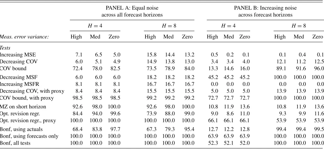
Turning to the power of the various forecast optimality tests, Table 2 reports the results of our simulations across the two scenarios. In the first scenario with equal noise across different horizons (Panel A), neither the MSE, MSF, MSFR nor decreas-ing covariance bounds have much power to detect deviations from forecast optimality. This holds across all three levels of measurement error. In contrast, the covariance bound on forecast revisions has very good power to detect this type of deviation from optimality, around 70%–99%, particularly when the short-horizon forecast, ˆYt|t−1, which is not affected by noise, is used
as the dependent variable. The covariance bound in Corollary 4 works so well because noise in the forecast increasesE[d2
t|hS,hL]
without affecting E[Ytdt|hS,hL], thereby making it less likely
thatE[2Ytdt|hS,hL−d
2
t|hS,hL]≥0 holds. The univariate optimal
revision regression in Equation (17) also has excellent power properties, notably when the dependent variable is the short-horizon forecast.
The scenario with additive measurement noise that increases in the horizon,h, is ideal for the decreasing MSF test since now the variance of the long-horizon forecast is artificially inflated in contradiction of Equation (7). Thus, as expected, Panel B ofTable 2shows that this test has very good power under this scenario: 45% in the case with four forecast horizons, rising to 100% in the case with eight forecast horizons. The MSE and MSFR bounds have essentially zero power for this type of deviation from forecast optimality. The covariance bound based on the predicted variable has power around 15% whenH=4, which increases to a power of around 90% whenH=8. The covariance bound with the actual value replaced by the short-run forecast in Equation (12), performs best among all tests, with power of 72% whenH =4 and power of 100% whenH=8. This is substantially higher than the power of the univariate
Table 1. Monte Carlo simulation of size of the inequality tests and regression-based tests of forecast optimality
H=4 H=8
Meas. error variance: High Med Zero High Med Zero
Tests
Increasing MSE 3.0 1.5 1.0 6.3 5.2 5.2
Decreasing COV 1.1 0.9 0.8 5.0 4.7 4.4
COV bound 1.8 1.4 1.2 0.0 0.0 0.0
Decreasing MSF 2.0 2.0 2.0 0.7 0.7 0.7
Increasing MSFR 0.1 0.1 0.1 4.4 4.4 4.4
Decreasing COV, with proxy 1.2 1.2 1.2 6.0 6.0 6.0
COV bound, with proxy 3.8 3.8 3.8 0.0 0.0 0.0
MZ on short horizon 10.8 11.9 13.6 10.8 11.9 13.6
Univar opt. revision regr. 10.2 9.7 9.8 11.5 10.2 9.4
Univar opt. revision regr., with proxy 10.8 10.8 10.8 9.5 9.5 9.5
Univar MZ, Bonferroni 12.5 12.9 18.2 18.4 19.1 22.4
Univar MZ, Bonferroni, with proxy 17.8 17.8 17.8 20.8 20.8 20.8
Vector MZ 33.2 31.5 28.9 92.2 89.9 83.5
Vector MZ, with proxy 20.7 20.7 20.7 68.6 68.6 68.6
Bonf, using actuals 3.0 2.7 2.5 8.0 7.5 8.5
Bonf, using forecasts only 3.0 3.0 3.0 7.0 7.0 7.0
Bonf, all tests 3.7 3.2 2.3 8.1 7.2 6.1
NOTES: This table presents the outcome of 1,000 Monte Carlo simulations of the size of various forecast optimality tests. Data are generated by a first-order autoregressive process with parameters calibrated to quarterly U.S. CPI inflation data, i.e.,φ=0.5, σ2
y=0.5, andµy=0.75.We consider three levels of error in the measured value of the target variable (high,
medium, and zero). Optimal forecasts are generated under the assumption that this process (and its parameter values) are known to forecasters. The simulations assume a sample of 100 observations and a nominal size of 10%. The inequality tests are based on the Wolak (1989) test and use simulated critical values based on a mixture of chi-squared variables. Tests labeled “with proxy” refer to cases where the one-period forecast is used in place of the predicted variable.
optimal revision regression test in Equation (17), which has power around 9%–11% when conducted on the actual values and power of 53%–66% when the short-run forecast is used as the dependent variable. For this case, ˆYt|t−hH is very poor,
but also very noisy, and so deviations from rationality can be relatively difficult to detect.
We also consider using a Bonferroni bound to combine var-ious tests based on actual values, forecasts only, or all tests. Results for these tests are shown at the bottom of Tables1and 2. In all cases we find that the size of the tests falls below the nominal size, as expected for a Bonferroni-based test. However, the power of the Bonferroni tests is high and is comparable to
Table 2. Monte Carlo simulation of power of the inequality tests and regression-based tests of forecast optimality
PANEL A: Equal noise PANEL B: Increasing noise across all forecast horizons across forecast horizons
H=4 H=8 H=4 H=8
Meas. error variance: High Med Zero High Med Zero High Med Zero High Med Zero
Tests
Increasing MSE 7.1 6.5 5.0 15.8 14.4 13.2 0.5 0.2 0.1 0.1 0.4 0.1 Decreasing COV 6.0 5.1 4.9 14.9 13.8 13.0 3.4 3.4 4.0 12.1 11.2 12.5 COV bound 72.4 78.0 82.5 73.5 78.9 84.0 13.3 14.6 16.0 89.1 91.6 96.0
Decreasing MSF 6.0 6.0 6.0 18.2 18.2 18.2 45.2 45.2 45.2 100.0 100.0 100.0 Increasing MSFR 8.1 8.1 8.1 16.7 16.7 16.7 0.0 0.0 0.0 0.0 0.0 0.0 Decreasing COV, with proxy 8.4 8.4 8.4 15.5 15.5 15.5 5.0 5.0 5.0 13.9 13.9 13.9 COV bound, with proxy 98.5 98.5 98.5 99.2 99.2 99.2 72.7 72.7 72.7 100.0 100.0 100.0
MZ on short horizon 92.6 98.0 100.0 92.6 98.0 100.0 10.8 11.9 13.6 10.8 11.9 13.6 Opt. revision regr. 84.4 94.0 99.6 73.9 88.0 99.0 9.0 8.6 11.0 9.3 9.9 11.6 Opt. revision regr., proxy 100.0 100.0 100.0 100.0 100.0 100.0 66.1 66.1 66.1 53.9 53.9 53.9
Bonf, using actuals 68.4 83.8 97.7 67.3 79.3 95.4 12.7 12.2 12.8 99.4 99.4 99.5 Bonf, using forecasts only 100.0 100.0 100.0 100.0 100.0 100.0 63.9 63.9 63.9 100.0 100.0 100.0 Bonf, all tests 100.0 100.0 100.0 100.0 100.0 100.0 52.3 52.1 52.0 100.0 100.0 100.0
NOTES: This table presents the outcome of 1,000 Monte Carlo simulations of the size of various forecast optimality tests. Data are generated by a first-order autoregressive process with parameters calibrated to quarterly U.S. CPI inflation data, i.e.,φ=0.5, σ2
y=0.5, andµy=0.75.We consider three levels of error in the measured value of the target variable
(high, medium, and zero). Optimal forecasts are generated under the assumption that this process (and its parameter values) are known to forecasters. Power is studied against suboptimal forecasts obtained when forecasts are contaminated by the same level of noise across all horizons (Panel A) and when forecasts are contaminated by noise that increases in the horizon (Panel B). The simulations assume a sample of 100 observations and a nominal size of 10%. Tests labeled “with proxy” refer to cases where the one-period forecast is used in place of the predicted variable.
the best of the individual tests. This suggests that it is possible and useful to combine the results of the various bound-based tests via a simple Bonferroni test.
It is also possible to combine these tests into a single omnibus test by stacking the various inequalities into a single large vector and testing whether the weak inequality holds for all elements of this vector. We leave this approach aside for two reasons: The first relates to concerns about the finite sample properties of a test with such a large number of inequalities relative to the number of available time series observations. The second relates to the interpretability of the omnibus test: by running each of the bound tests separately we can gain valuable information into the sources of forecast suboptimality, if present. An omnibus bound test would, at most, allow us to state that a given sequence of forecasts is not optimal; it would not provide information on the direction of the suboptimality.
We also used the bootstrap approaches of White (2000) and Hansen (2005) to implement the tests of forecast rationality based on multi-horizon bounds in our simulations. We found that the finite sample size and power from those approaches are very similar to those presented in Tables1and 2, and so we do not discuss them separately here.
In conclusion, the covariance bound test performs best among all the second-moment bounds. Interestingly, it generally per-forms much better than the MSE bound which is the most com-monly known variance bound. Among the regression tests, ex-cellent performance is found for the univariate optimal revision regression, particularly when the test uses the short-run forecast as the dependent variable. This test has good size and power properties and performs well across both deviations from fore-cast efficiency. Across all tests, the covariance bound and the univariate optimal revision regression tests are the best indi-vidual tests. Our study also finds that Bonferroni bounds that combine the tests have good size and power properties.
6. EMPIRICAL APPLICATION
As an empirical illustration of the forecast optimality tests, we next evaluate the Federal Reserve Greenbook forecasts of quarter-over-quarter rates of change in GDP, the GDP deflator, and CPI. Data are from Faust and Wright (2009), who extracted the Greenbook forecasts and actual values from real-time Fed publications, extended by 4 years. We use quarterly observations of the target variable over the period from 1980Q1 to 2004Q4, a total of 100 quarters. The forecast series begin with the current quarter and run up to five quarters ahead in time, that is,h= 0,1,2,3,4,5. All series are reported in annualized percentage points. If more than one Greenbook forecast is available within a given quarter, we use the earlier forecast. If we start the sample when a full set of six forecasts is available, then we are left with 95 observations. This latter approach is particularly useful for comparing the impact of the early part of our sample period, when inflation volatility was high.
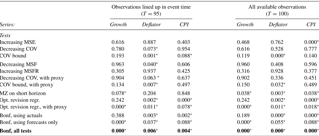
The results of our tests of forecast rationality are reported inTable 3. Panel A shows the results for the common sample (1981Q2–2004Q4) that uses 95 observations, and represents our main empirical results. For GDP growth, we observe a strong rejection of internal consistency via the univariate optimal revi-sion regresrevi-sion using the short-run forecast as the target variable, Equation (20), while none of the bound tests reject. For the GDP deflator, several tests reject forecast optimality. In particular, the tests for decreasing covariance between the forecast and the ac-tual, the covariance bound on forecast revisions, a decreasing mean squared forecast, and the univariate optimal revision re-gression all lead to rejections. Finally, for the CPI inflation rate we find a violation of the covariance bound, Equation (12), and a rejection through the univariate optimal revision regression. For all three variables, the Bonferroni combination test rejects multi-horizon forecast optimality at the 5% level.
Table 3. Forecast rationality tests for Greenbook forecasts
Observations lined up in event time All available observations
(T=95) (T=100)
Series: Growth Deflator CPI Growth Deflator CPI
Tests
Increasing MSE 0.616 0.887 0.403 0.468 0.762 0.000∗
Decreasing COV 0.780 0.073∗ 0.954 0.616 0.528 0.777
COV bound 0.193 0.001∗ 0.088∗ 0.119 0.000∗ 0.140
Decreasing MSF 0.963 0.040∗ 0.606 0.960 0.408 0.596
Increasing MSFR 0.305 0.937 0.425 0.316 0.928 0.377
Decreasing COV, with proxy 0.904 0.063∗ 0.637 0.902 0.336 0.451
COV bound, with proxy 0.134 0.007∗ 0.497 0.150 0.032∗ 0.489
MZ on short horizon 0.078∗ 0.204 0.848 0.038∗ 0.003∗ 0.038∗
Opt. revision regr. 0.242 0.002∗ 0.000∗ 0.242 0.002∗ 0.000∗
Opt. revision regr., with proxy 0.000∗ 0.011∗ 0.078∗ 0.000∗ 0.011∗ 0.018∗
Bonf, using actuals 0.388 0.003∗ 0.002∗ 0.189 0.000∗ 0.000∗
Bonf, using forecasts only 0.000∗ 0.037∗ 0.088∗ 0.000∗ 0.055∗ 0.088∗
Bonf, all tests 0.000∗ 0.006∗ 0.004∗ 0.000∗ 0.000∗ 0.000∗
NOTES: This table presentsp-values from inequality and regression tests of forecast rationality applied to quarterly Greenbook forecasts of GDP growth, the GDP deflator and CPI Inflation. The sample covers the period 1980Q1–2004Q4. Six forecast horizons are considered, (h=0, 1, 2, 3, 4, 5 quarters) and the forecasts are aligned in event time. The inequality tests are based on the Wolak (1989) test and use critical values based on a mixture of chi-squared variables. Tests labeled “with proxy” refer to cases where the shortest-horizon forecast forecast is used in place of the target variable in the test.P-values less than 0.10 are marked with an asterisk. In order, the tests listed in the rows correspond to Corollary 1(a), 3(a), 4(a), 2, 1(b), 3(b), 4(b), 6, 7, 8(c).
5 4 3 2 1 0 0
2 4 6
8 Growth
Forecast horizon
V
ariance
5 4 3 2 1 0
0 1 2 3
4 Deflator
Forecast horizon
V
ariance
5 4 3 2 1 0
0 1 2 3 4
5 CPI
Forecast horizon
V
ariance
MSE V[forecast] V[actual]
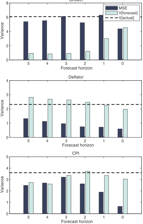
Figure 1. Mean squared errors and forecast variances, for U.S. GDP deflator, CPI inflation and GDP growth. (Color figure available online.)
Faust and Wright (2008) pointed out that forecasts from cen-tral banks are often based on an assumed path for the policy interest rate, and forecasts constructed using this assumption may differ from the central bank’s best forecast of the target variable. Ignoring this conditioning can lead standard tests to over- or under-reject the null of forecast rationality. We leave the extension of our bound-based tests to conditional forecasts for future work.
Figures1and 2 illustrate the sources of some of the rejections of forecast optimality. For each of the series, Figure 1 plots the mean squared errors and variance of the forecasts. Under the null of forecast optimality, the forecast and forecast error should be orthogonal and the sum of these two components should be constant across horizons. Clearly, this does not hold here, particularly for the GDP deflator and CPI inflation series. In fact, the variance of the forecast increases in the horizon for the GDP deflator, and it follows an inverseU-shaped pattern for CPI inflation, both in apparent contradiction of the decreasing forecast variance property established earlier.
Figure 2plots mean squared forecast revisions and the co-variance between the forecast and the actual against the forecast horizon. Whereas the mean squared forecast revisions are mostly increasing as a function of the forecast horizon for the two in-flation series, for GDP growth we observe the opposite pattern, namely a very high mean squared forecast revision at the one-quarter horizon, followed by lower values at longer horizons. In the right panel, we see that while the covariance between the forecast and the actual is decreasing in the horizon for GDP growth and CPI, for the GDP deflator it is mildly increasing, a contradiction of forecast rationality.
The Monte Carlo simulations are closely in line with our em-pirical findings. Rejections of forecast optimality come mostly from the covariance bound in Equation (12) and the univariate optimal revision regressions in Equations (17) and (20). More-over, for GDP growth, a series with greater measurement errors
5 4 3 2 1 0
0 1 2 3 4 5 6 7
forecast horizon Mean squared forecast revisions
Growth CPI Deflator
5 4 3 2 1 0
0 0.5 1 1.5 2 2.5 3 3.5 4
forecast horizon
Covariance between forecast and actual
Growth CPI Deflator
Figure 2. Mean squared forecast revisions (left panel) and the covariance between forecasts and actuals, for U.S. GDP deflator, CPI inflation and GDP growth. (Color figure available online.)