Full Terms & Conditions of access and use can be found at
http://www.tandfonline.com/action/journalInformation?journalCode=ubes20
Download by: [Universitas Maritim Raja Ali Haji] Date: 11 January 2016, At: 22:36
Journal of Business & Economic Statistics
ISSN: 0735-0015 (Print) 1537-2707 (Online) Journal homepage: http://www.tandfonline.com/loi/ubes20
A Balanced System of U.S. Industry Accounts
and Distribution of the Aggregate Statistical
Discrepancy by Industry
Baoline Chen
To cite this article: Baoline Chen (2012) A Balanced System of U.S. Industry Accounts and Distribution of the Aggregate Statistical Discrepancy by Industry, Journal of Business & Economic Statistics, 30:2, 202-211, DOI: 10.1080/07350015.2012.669667
To link to this article: http://dx.doi.org/10.1080/07350015.2012.669667
Accepted author version posted online: 03 Apr 2012.
Submit your article to this journal
Article views: 144
A Balanced System of U.S. Industry Accounts
and Distribution of the Aggregate Statistical
Discrepancy by Industry
Baoline C
HENBureau of Economic Analysis, Washington, DC 20230 ([email protected])
This article describes and illustrates a generalized least squares (GLS) method that systematically incorpo-rates all available information on the reliability of initial data in the reconciliation of a large disaggregated system of national accounts. The GLS method is applied to reconciling the 1997 U.S. Input-Output and Gross Domestic Product (GDP)-by-industry accounts with benchmarked GDP estimated from expendi-tures. The GLS procedure produced a balanced system of industry accounts and distributed the aggregate statistical discrepancy by industry according to the estimated relative reliabilities of initial estimates. The study demonstrates the empirical feasibility and computational efficiency of the GLS method for large accounts reconciliation.
KEY WORDS: Accounts reconciliation; Data reliability; GLS estimation.
1. INTRODUCTION
Systems of national accounts are constructed using data from a variety of sources, and, thus, typically contain various types of measurement errors. Initial estimates of national accounts items rarely satisfy all the identities and restrictions of the counting system. The usual reconciliation procedure uses ac-counting identities from different parts of the system to reduce accounting discrepancies as much as possible and to record the residuals between the major aggregates. For example, the Bu-reau of Economic Analysis (BEA) publishes estimates of U.S. Gross Domestic Product (GDP) and Gross Domestic Income (GDI), which are conceptually equivalent, but in fact, are incon-sistent. The difference between GDP and GDI is the estimated aggregate statistical discrepancy. Currently statistical discrep-ancy is estimated only at the aggregate level, not by industry or by expenditure category. Lack of information on sub-aggregate discrepancies hinders a good understanding of the sources of aggregate inconsistency and makes it difficult to identify im-provements in the source data and estimation methods, which might reduce statistical discrepancies.
Reconciliation in the system of national accounts is often conducted through updating or balancing input-output and other economic accounts matrices. Traditional balancing procedures are purely numerical and often conducted manually. Automatic balancing using numerical procedures, such as the Iterative
Proportional Fitting or Raking (Deming and Stephan 1940),
is sometimes conducted in final stages of balancing. Traditional procedures are often considered arbitrary and unjustified either by economic or statistical reasoning. Instead, Stone, Meade, and
Champernowne (1942) proposed a generalized least squares
(GLS) method for reconciling national accounts according to data reliability determined by measurement errors. GLS rec-onciliation has two empirical advantages. First, it has a firm Bayesian foundation which allows information on the relative reliability of initial data to be used formally in the reconciliation process. Using the GLS method, reconciliation is achieved by trading off relative data uncertainty in the system in order to
adjust initial estimates so that they satisfy the accounting con-straints. Second, it is flexible in that it may be applied
hierarchi-cally (Dagum and Cholette2006) and can easily accommodate
additional constraints (Barker, van der Ploeg, and Weale1984).
However, in the past, it was impractical to use the GLS method in large accounting systems because of its large computational
requirements. Thus, the RAS method (Bacharach 1965)
be-came very popular for balancing input-output matrices. The RAS method, however, does not allow varying degrees of un-certainty in initial estimates and constraints, provides dubious economic interpretation of the balancing results, and requires a large number of iterations for convergence. As an alternative to the GLS procedure proposed by Stone, Meade, and
Champer-nowne (1942), Byron (1978) introduced a more efficient
pro-cedure based on the conjugate gradient algorithm and, thus, made it empirically feasible to implement the GLS method in large accounting systems. The GLS reconciliation method has
since been developed further (Stone1984; van der Ploeg1982a,
1982b; Bartholdy1991; Weale1992), and its empirical
feasibil-ity has been demonstrated by van der Ploeg (1982a,1988) and
Barker, van der Ploeg, and Weale (1984).
Despite these developments, the GLS reconciliation method has not been adopted widely by national accounting systems,
since its first inception by Byron (1978), for two reasons. The
first previous problem, the need for large computer memory, is no longer a constraint. The second problem was, and still is, insufficient objective information on the reliability of initial data. In previous applications, reliability of initial data was set
subjectively (van der Ploeg1982a; Barker, van der Ploeg, and
Weale1984; Beaulieu and Bartelsman2004). Of course,
recon-ciliation based on subjectively set reliabilities will be subjective, not objective. The difficulty in obtaining sufficient objective in-formation on the reliability of initial data had greatly prevented
In the Public Domain Journal of Business & Economic Statistics
April 2012, Vol. 30, No. 2 DOI:10.1080/07350015.2012.669667
202
implementation of GLS reconciliation in national accounting systems more than six decades after it was first introduced. The few countries (e.g., Australia, Canada, and UK) that pub-lish reconciled annual estimates of GDP derive it as an average of GDP estimated using production, expenditures, and income approaches.
The objective of this study is to illustrate, using U.S. data, the empirical feasibility of incorporating all available objective information on the reliability of initial data in order to reconcile a large system of national accounts using the GLS method and to distribute the aggregate statistical discrepancy by industry.
The GLS method is applied to reconciling the 1997 U.S. Input-Output (IO) and GDP-by-industry accounts with the expenditure-based GDP at the level of detail of 65 industries (see the Appendix), 69 commodity groups, 3 value-added (VA) components, and 13 final demand categories, including exports and imports. Before reconciliation, initial estimates in the IO accounts were imbalanced; initial estimates of VA from the IO accounts and from the GDP-by-industry accounts were incon-sistent; and initial estimates of VA from neither set of accounts were consistent with the expenditure-based GDP.
The GLS procedure reconciled the accounts and distributed the aggregate statistical discrepancy by industry according to the estimated reliabilities of initial estimates. Compared with results from traditional methods that often obtain economi-cally unconvincing results, the GLS estimates reveal relative uncertainties of the initial source data. Less reliable initial data resulted in larger % adjustments through reconciliation than more reliable initial data. In a previous study (Beaulieu and
Bartelsman 2004), the aggregate discrepancy was distributed
to industries according to the industry shares of total GDP, implying that larger industries account for larger shares of the aggregate discrepancy. In contrast, the GLS estimates of the in-dustry statistical discrepancies trace the aggregate discrepancy to its sources based on the reliability of initial data. This study demonstrates that it is empirically feasible and computationally efficient to implement the GLS method in a large system of national accounts according to estimated relative reliabilities of initial data. A major merit of the GLS method, compared with traditional methods, is that it is transparent and, hence, straightforwardly replicable for given data.
The plan for the article is as follows. Section 2 discusses major reliability problems in the 1997 U.S. industry accounts data. Section 3 describes the GLS method and construction of a covariance matrix for the U.S. data. Section 4 discusses reliability of initial data. Section 5 presents reconciled results and discusses them from the prospective of a sensitivity test. Section 6 concludes the article.
2. MAJOR PROBLEMS OF 1997 U.S. INDUSTRY ACCOUNTS DATA
U.S. industry accounts measure GDP-by-industry using pro-duction and income data. In the IO accounts, GDP of an industry is the VA of the industry measured as the difference between values of gross output and values of intermediate inputs. VA of all industries must sum to GDP measured by expenditures. In the GDP-by-industry accounts, VA of an industry measures the industry’s total income and VA of all industries sum to GDI.
In theory, GDP estimated from production and income data should equal expenditure-based GDP but this does not happen in practice. For the 1997 accounts, inconsistencies in estima-tion of GDP using producestima-tion, income, and expenditure data were due to four major sources of error in the initial IO and GDP-by-industry data.
The first major source of error was due to differences in def-initions and classifications of variables, and in data collection and estimation methods used by different statistical agencies. For the 1997 benchmark IO accounts, initial data on gross out-put and on intermediate inout-puts were compiled mostly using data from the 1997 Economic Census and surveys conducted by the U.S. Bureau of the Census. The GDP-by-industry accounts contain industry VA estimates based on data on compensation, taxes, and subsidies, and gross operating surplus (GOS) which measures industry profits. The primary source data on com-pensation, taxes and subsidies were from the Bureau of Labor Statistics (BLS) and BEA. A major portion of GOS data came from Statistics of Income (SOI) data of the Internal Revenue Ser-vices (IRS). Other data, from the Federal Reserve Board, from other government agencies, and from private trade companies, were also used in both accounts.
The second major source of error was sampling and nonsam-pling errors in the source data. The Census Bureau and SOI provide information on sampling errors, for their published es-timates, in terms of coefficients of variation (CV), defined as a standard deviation divided by a mean. Nonsampling errors were either due to inconsistencies in definition and classifi-cation of variables between data collection agencies and the national accounts or due to problems in data collection and processing methods. For example, source data in both sets of the accounts suffered from nonsampling errors such as double counting, misreporting, omissions, misallocations, and
misspec-ifications (ASR Analytics2005).
The third major source of error came from adjustments aimed to correct nonsampling errors in source data. However, adjust-ments themselves introduced additional uncertainty, because some were based on out-of-date methods and some were made judgmentally.
The fourth major source of error was the aggregate statistical discrepancy, which, recorded as a separate item in the GDP-by-industry accounts, was a major inconsistency to be removed.
3. GENERALIZED LEAST SQUARES METHOD FOR RECONCILING NATIONAL ACCOUNTS
Following Byron (1996), this section describes a GLS method
for reconciling a set of national accounts. Subsection 3.1 de-scribes the GLS method in general. The three inputs to the method are initial estimates of variables to be adjusted, covari-ances which measure their accuracy, and variables to be held fixed at the initial estimates and not to be adjusted. Subsec-tion 3.2 discusses available sample informaSubsec-tion for setting the measurement-accuracy covariance matrix to be used in the ap-plication with U.S. data in Section 5.
3.1 The General GLS Problem
Letαdenote the n × 1 vector of true, nonstochastic, and
unknown values of variables in a linear system of national
204 Journal of Business & Economic Statistics, April 2012
accounts. The system consists ofm+ 1 accounts, andαis said
to be reconciled when it satisfies the linear accounting system
Hα=β. (1)
System (1) imposesm(<n) independent linear constraints
on thenvariables inα, for a givenm ×nmatrixHand a given
m × 1 vectorβ. Independence of the constraints means thatH
has full row rankm, the elements ofHare either 0 or ±1, and
in the overall accounting, there is usually one more constraint
not included in (1) so as to preserveH’s full row rank. Them +
1th account is redundant because it follows from adding up the first m accounts.
Let α0 denote an initial, unreconciled, estimate of α,
pro-duced by a statistical agency, so that errore0 =Hα0 −β =
0. Following Byron (1996), suppose thatα0is considered as a
stochastic and unbiased estimate of trueα, with positive definite
covariance matrix. The GLS method computes an adjusted
and reconciled estimate denoted by α∗ which is as close as
possible toα0. Letr=α∗ −α0denote the adjustment from
rank andis positive definite, then the problem has the unique
solution:
α∗=α0−H′(HH′)−1(Hα0−β). (3)
If trueαis reconciled and initialα0is unbiased, then revised
α∗is also an unbiased estimate of trueα(Byron 1996). The idea
of weighting by−1in objective function (2) is to induce small
adjustments of accurate initial estimates with small variances in an adjusted and reconciled accounting system and vice versa for inaccurate initial estimates. Optimal adjustment rule (3) has the Bayesian interpretation of being drawn from a posterior
distribution ofα(van der Ploeg 1982b).
Because (3) is based onα0being unbiased, one would like
to test this assumption statistically. Supposing α0 is normally
distributed, Byron (1996) proposed testing this assumption with
the quadratic formg=(α∗−α0
)′H′(H−1H′)−1H
(α∗−α0
),
distributed chi-squared withmdegrees of freedom. As usual, a
large and significant value of grejects the null hypothesis that
α0is unbiased. Normality is a reasonable assumption for initial
estimates in national accounts (Bryon 1996). In the application
in Section 5,g=159.9 and m=134 imply thatghas apvalue
of 0.937, which does not reject unbiasedness of α0at the 5%
significance level.
3.2 Settingfor U.S. National Accounts Data
In the application in Section 5 with U.S. data, there are 134
independent accounting constraints (rows ofH) and 9165
vari-ables (columns ofH and elements of α). The variables to be
adjusted inαare gross output, intermediate inputs, and VA. In
addition, not to be adjusted final expenditures, including exports
and imports, are inβ. The GLS method is applied to the 1997 IO
and GDP-by-industry data, conditional on the 2003 benchmark revision of final expenditures, with 134 independent accounting
constraints in Equation (1) reflecting 65 industry and 69 com-modity constraints. As usual, there is one more overall constraint equating total industry VA with total expenditure-based GDP,
which is excluded from (1) in order to preserveH’s full row rank.
Ideally, we would like all variables, including final expendi-tures, to be part of the reconciliation. However, in the application
in Section 5, final expenditures were held fixed inβand were not
in adjustedα∗, because BEA required final expenditures to be
unadjusted and because a main purpose of the application is to demonstrate the GLS method in the closest proximity to actual practice. BEA required final expenditures to be unadjusted in or-der to conform to its policy of keeping benchmark input-output accounts, constructed after a comprehensive GDP revision, con-sistent with already released benchmark-revised GDP. BEA did this also because some BEA studies found expenditure-based GDP to be quite reliable in the sense that historical revisions
were small (Fixler and Grimm2005). If in the application, final
expenditures were included inα, thenβwould be zero and final
expenditures would be explicitly considered at least somewhat
inaccurate in the sense of having positive variances in.
In the application in Section 5,is restricted to be
diago-nal, with positive diagonal elements,ωii >0, set to estimated
variances of elements inα0. Ideally, survey data would provide
enough information to estimate all elements in. However, U.S.
survey data underlying the data used in Section 5 provided only
information to estimate variances in. In particular, only CV for
IO data from the Census Bureau and for VA data from SOI were available and were converted to estimated variances by multi-plying them by sample means and squaring. Accordingly, in the application, data were considered inaccurate according to their
estimated variances. Restrictingto be a diagonal matrix of
estimated variances is standard practice in least-squares-based reconciliation using data from surveys (Dagum and Cholette
2006), because only relative variances play a role in
determin-ing the adjustments.
It is possible to establish an upper bound of the norm of
ad-justmentr=α∗−α0in terms of the norm of errore
0=Hα0−
βand the norm of the covariance matrix. In particular, ifis
diagonal, then the upper bound of the norm ofrdepends on the
ratio of the largest to the smallest diagonal elements of, which
implies that adjustments have a smaller upper bound if the vari-ables to be adjusted have equal uncertainties and have a larger upper bound if the variables have different relative uncertainties.
See Chen (2006) for details of this upper bound analysis.
4. RELIABILITY OF INITIAL DATA
This section discusses how reliability of initial estimates was determined. Because initial data come from various sources, an initial estimate consists of two parts, source data and ad-justments, where source data are from official data collection agencies and adjustments aim to correct nonsampling errors in source data. Adjustments vary between variables and across industries. In the 1997 data, adjustments in gross output, inter-mediate inputs, and VA were, respectively, 14%, 9.3%, and 7.5% of the total initial estimates. Adjustments in VA were mostly in the GOS component of VA, amounting to about 36% of total initial GOS estimates.
Reliability of source data is usually measured by estimated variances based on published estimates and CVs provided by statistical agencies. Data from the Economic Census have no assigned sampling errors, and, thus, have zero assigned CVs. Administrative data, such as salaries, wages, taxes, and subsi-dies, are provided by regulatory agencies and, thus, are treated like data from the Economic Census.
Estimating reliability of adjustments is less straightforward, because there is inadequate information about the uncertainty
in adjustments. Stone, Meade, and Champernowne (1942)
ad-dressed this issue and suggested that in the absence of standard errors, margins of error may be set judgmentally by experienced analysts. Depending on how they were compiled, adjustments fell into three categories in decreasing order of reliability,
de-noted byθ=(1, 2, 3). Letα0i,A
θdenote an adjustment item of the
ith element inα0of categoryθ, and letcdenote the minimum
CV of the three categories of adjustments. The subjective CV
ofαi,A0
θ is, then, computed as
CV
αi,A0
θ
=c·θ . (4)
The subjective standard error of an adjustment is, thus, the product of the subjective CV and the estimate of adjustment. Based on the knowledge of experienced analysts, Equation (4) is used to differentiate among varying degrees of uncertainty in adjustments. Here, CVs of adjustments in the three categories are 0.1, 0.2, and 0.3. The minimum subjective CV of 0.1 is the average CV of detailed data items from surveys from the Economic Census.
Thus, reliability of an initial estimate inα0, in the sense of its
diagonal element of, is measured by the sum of variances of
the source data and the adjustments,
ωii =var
i,A refer to the source data and adjustment
components of theith item inα0, andα0i,A=3
1α 0
i,Aθ.
The CVs from statistical agencies should be acceptable, be-cause they are estimated using survey data. Subjective CVs, not based on survey data, are more questionable. In Section 5, we check the sensitivity of the results with respect to different values of subjective CVs, holding fixed the objective data-determined CVs. We consider five different sets of subjective CVs based
onc=(0.05, 0.1, 0.15, 0.2, 0.25), which, using Equation (4),
imply five sets of subjective CVs of the three categories for the sensitivity test (0.5, 0.1, 0.15), (0.1, 0.2, 0.3), (0.15, 0.3, 0.45), (0.2, 0.4, 0.6), and (0.25, 0.5, 0.75). We consider (0.1, .2, .3) to be the baseline case, because these values reflect the knowledge of experienced analysts.
In Section 5, we contrast this uncertainty measure with a so-called neutral variant, defined as the square of an initial
es-timate, ωii =(αi0)
2(Barker, van der Ploeg, and Weale1984).
The neutral variant measure is motivated by the idea that large initial estimates imply large discrepancies in the accounts. Rec-onciling different accounts using neutral variants is equivalent to assuming that all initial estimates have the same degree of uncertainty.
5. A BALANCED SYSTEM OF ACCOUNTS
This section discusses the GLS reconciliation using the 1997 U.S. IO accounts, GDP-by-industry accounts, and final expenditures from the 2003 GDP benchmark revision. In the reconciled system of accounts, the IO accounts are balanced, the IO and GDP-by-industry accounts are reconciled with expenditure-based GDP. Subsection 5.1 compares two sets of reconciled accounts based on estimated relative reliabilities and neutral variants of initial estimates. Subsection 5.2 com-pares adjustments in initial estimates from reconciliation and estimated statistical discrepancies by industry. Subsection 5.3 reports the results of the sensitivity test of balanced estimates. Subsection 5.4 discusses implications of the reconciliation.
5.1 Balanced Estimates of the Input-Output Accounts
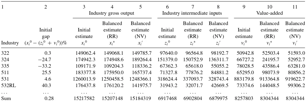
Tables 1 and 2 contain initial estimates and two sets of balanced estimates in the IO accounts for a subset of the
Table 1. Initial and balanced estimates by industry (millions of dollars)
1 2 3 4 5 6 7 8 9 10 11
Industry gross output Industry intermediate inputs Value-added
Balanced Balanced Balanced Balanced Balanced Balanced Initial Initial estimate estimate Initial estimate estimate Initial estimate estimate
gap estimate (RR) (NV) estimate (RR) (NV) estimate (RR) (NV) Industry (xi0−(zi0 + vi0))% xi0 xi∗ xi′ zi0 zi∗ zi′ vi0 vi∗ vi′
322 0.3 149062.4 149068.1 149785.7 97640.0 96564.8 98192.7 50942.8 52503.4 51593.0 324 −24.7 174942.3 174948.6 189264.4 151379.0 150752.9 136311.7 66727.2 24195.7 52952.7 335 −33.2 109171.9 109204.3 118336.2 67362.3 65618.0 55055.2 78028.5 43586.4 63281.0 511 25.5 183377.8 175950.0 165737.4 71327.8 77876.2 84881.2 65295.0 98073.9 80856.2 531 4.6 1260013.9 1250458.5 1248366.1 318624.4 337093.7 328743.4 883179.8 913364.8 919622.7 532RL 40.3 176437.8 176120.2 141975.7 31943.2 32071.7 42669.5 73374.6 144048.5 99306.2
. . . .
Sum 0.28 15217582 15207148 15184319 6917468 6902804 6879975 8257803 8304344 8304344
NOTE: Col. 2 shows % initial gaps between gross output (xi) and total inputs (zi+vi); col. 3–5, 6–8, and 9–11 are initial and balanced estimates of gross output, intermediate inputs, and value-added based, respectively, on relative reliabilities (RR) and neutral variants (NV). Industries are listed using North American Industry Classification System (NAICS) codes (see the Appendix).
206 Journal of Business & Economic Statistics, April 2012
Table 2. Initial and balanced estimates by commodity (millions of dollars)
1 2 3 4 5 6 7 8 9
Commodity gross output Commodity intermediate inputs Final uses
Balanced Balanced Balanced Balanced Initial and Initial Initial estimate estimate Initial estimate estimate balanced % gap estimate (RR) (NV) estimate (RR) (NV) estimate Commodity (xk−(zk + yk))% xk0 xk∗ xk′ zk0 zk∗ zk′ yk0
324 −0.37 173625.9 173644.9 185042.6 118089.5 117467.6 128865.3 56177.3 335 −0.13 107525.7 107558.1 115068.9 75599.5 75492.6 83003.4 32065.5 481 8.65 124418.0 114880.1 120991.8 53652.3 54878.2 60989.9 60001.9 483 −2.30 24633.5 24633.5 25004.7 7165.0 6599.2 6970.4 18034.3 487OS −6.65 83861.2 83865.7 88136.1 73249.8 67680.1 71950.5 16185.6 532RL −0.02 246249.3 245658.6 221341.9 154894.8 154259.2 129942.5 91399.4
. . . .
Sum −0.03 15217582 15207148 15184319 6917468 6902804 6879975 8304344
NOTE: Col. 2 shows initial % gaps between gross output (xk) and total inputs (zk+yk) by commodity; col. 3–5 and 6–8 contain initial and balanced estimates of commodity gross output and intermediate inputs based, respectively, on relative reliabilities (RR) and neutral variants (NV); and col. 9 shows initial (not adjusted) final uses. Commodities are listed by NAICS codes.
65 industries and 69 commodities based on estimated relative reliabilities and neutral variants of initial estimates. Initial and balanced estimates for all 65 industries and 69 commodities can
be found inTables 1and2in Chen (2006). Column 2 in both
tables shows inconsistencies or gaps in percentages between initial estimates of gross outputs and total inputs. Initial gaps reflect varying degrees of violation of accounting constraints across industries and commodities. Because initial estimates of final uses from the IO accounts were very close to final expendi-tures from the 2003 benchmark GDP, initial gaps by commodity are in general much smaller than initial gaps by industry.
Initial estimates of each variable are compared with balanced estimates based on relative reliabilities and neutral variants. Sums of balanced estimates of gross output and intermediate
inputs of all industries shown in the last row ofTable 1match
those of balanced estimates of gross output and intermediate
inputs of all commodities shown in the last row ofTable 2, and
sums of balanced estimates of VA shown inTable 1match the
sum of unadjusted final uses shown inTable 2, indicating that the
IO accounts are balanced, and that the IO and GDP-by-industry accounts are reconciled with expenditure-based GDP.
We observe two significant features of the balanced estimates. First, if an industry or a commodity has a large initial gap, ad-justments will be large at least for some variables (e.g., industry 324 and 335). Second, the sizes of adjustments can be dispropor-tional in gross output, intermediate inputs, and VA for reconcili-ation based on relative reliabilities, whereas adjustments tend to be more proportional for reconciliation based on neutral variants (e.g., industry 511 and 532RL; commodity 335 and 481).
5.2 Adjustments by Variable and Statistical Discrepancy by Industry
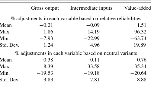
The second feature of the balanced estimates is depicted in
Figure 1andTable 3. In accounts reconciled by relative relia-bilities of initial estimates, the absolute means and standard de-viations of % adjustments of the 65 industries are much smaller for gross output and intermediate inputs than for VA, because
their initial estimates, compiled mostly from surveys from the Economic Census and a smaller portion of category 3 adjust-ments to correct nonsampling errors, are more reliable, whereas initial estimates of GOS in VA, compiled using SOI estimates, which have larger sampling errors and a larger portion of cat-egory 3 adjustments, are less reliable. By contrast, in accounts reconciled by neutral variants, relative sizes of initial estimates affect sizes of adjustments. Despite large varying degrees of relative reliabilities, differences in absolute means and standard deviations of % adjustments are much smaller.
Table 4shows statistical discrepancies distributed to a subset of the 65 industries, computed as adjustments in VA estimates in the GDP-by-industry accounts. Distribution of the aggregate
statistical discrepancy to all 65 industries can be found in
Ta-ble 4in Chen (2006). Columns 2 and 3 show initial gaps, in levels and percentages, between estimates of VA from IO and GDP-by-industry accounts. Estimated industry statistical dis-crepancies based on relative reliabilities and neutral variants are in the middle and right panels. Two notable features echo those
observed fromTables 1and2. First, sizes of initial gaps in VA
estimates between the two accounts affect sizes of discrepancies by industry (e.g., industry 213 and 514). Second, if accounts are reconciled according to relative reliabilities, relative variances of
Table 3. Summary statistics of % adjustments of 65 industries based on relative reliabilities and neutral variants
Gross output Intermediate inputs Value-added
% adjustments in each variable based on relative reliabilities
Mean −0.21 −0.09 1.51
Max. 1.86 14.19 96.32
Min. −7.93 −22.99 −63.74 Std. Dev. 1.24 4.96 19.89
% adjustments in each variable based on neutral variants
Mean −0.38 −0.11 0.76
Max. 8.39 33.58 35.34
Min. −19.53 −19.18 −20.64 Std. Dev. 3.83 7.81 8.88
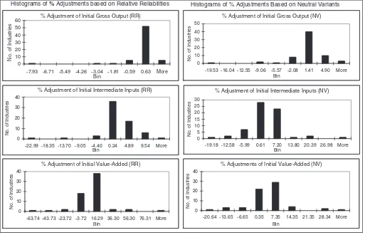
Histograms of % Adjustments based on Relative Reliabilities Histograms of % Adjustments Based on Neutral Variants
-7.93 -6.71 -5.49 -4.26 -3.04 -1.81 -0.59 0.63 More Bin
% Adjustment of Initial Intermediate Inputs (RR)
0 10 20 30 40
-22.99 -18.35 -13.70 -9.05 -4.40 0.24 4.89 9.54 More Bin
-63.74 -43.73 -23.72 -3.72 16.29 36.30 56.30 76.31 More Bin
% Adjustment of Initial Intermediate Inputs (NV)
0
-19.18 -12.58 -5.99 0.61 7.20 13.80 20.39 26.98 More Bin
-19.53 -16.04 -12.55 -9.06 -5.57 -2.08 1.41 4.90 More Bin
-20.64 -13.65 -6.65 0.35 7.35 14.35 21.35 28.34 More Bin
Figure 1. Distribution of % adjustments by industry in gross output, intermediate inputs, and value-added. NOTE: An adjustment measures the difference between balanced and initial estimate. Evenly distributed bin intervals, computed as the difference between the maximum and minimum values divided by the number of bins, are used. The numbers in the horizontal axis represent the highest values of the intervals. In comparison with adjustments based on neutral variants, adjustments based on relative reliabilities show smaller means and dispersions in the % adjustments in initial estimates of gross output and intermediate inputs, but show larger mean and dispersion in the % adjustments in initial VA estimates, reflecting lower reliability in initial VA estimates.
initial estimates primarily determine discrepancies by industry (e.g., industry 324 and 532RL). To the contrary, if reconciliation is based on neutral variants, relative shares of industry VA of total GDP determine the distributions (e.g., industry 485 and 531).
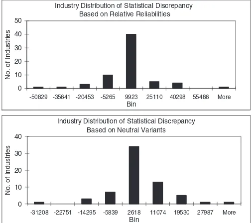
In contrast to the distribution based on neutral variants,
Fig-ure 2andTable 5depict a more dispersed distribution of the aggregate discrepancy with larger estimated industry discrepan-cies in the accounts reconciled according to relative reliabilities of initial data.
Table 4. Estimated statistical discrepancy distributed by industry (millions of dollars and %)
1 2 3 4 5 6 7 8 9
Initial estimates Estimates based on relative reliability Estimates based on neutral variants
Industry SD Industry SD VA share Initial Initial VA Industry as % of Relative Industry as % of of GDP VA gap gap (%) SD initial VA variance SD initial VA (%) Industry (xi0−zi0)−vi0 [(xi0−zi0)−vi0]% vi∗−vi0 (vi∗−vi0)/vi0 var(vi0)/ var(xi0−zi0) vi′−vi0 (vi′−vi0)/v0 (vi′/GDP)%
213 −6268.0 −34.3 −4409.5 −31.9 1.4 −3485.6 −19.1 0.2 324 −43163.9 −64.7 −42531.5 −175.8 71.5 −13774.5 −20.6 0.6
485 4080.3 33.7 2861.2 19.1 0.6 1567.8 13.0 0.2
514 11680.9 62.8 9275.9 33.3 13.2 4283.9 23.0 0.3
531 58209.6 6.6 30185.0 3.3 0.3 36442.9 4.1 11.1
532RL 71120.0 96.9 70673.9 49.1 95.4 25931.6 35.3 1.2
. . . .
Sum 42310.9 0.05 46541 100 46541 100
NOTE: Initial VA gap equals the difference between VA estimated by IO accounts computed as the residual of gross output minus intermediate inputs, (xi−zi), and VA estimated by GDP-by-industry accounts (vi), wherexiandziare industry gross output and intermediate inputs. The middle and right panels display results based on relative reliabilities and neutral variants. Cols. 4 and 7 show statistical discrepancy (SD) distributed by industry in millions of dollars; cols. 5 and 8 show industry SD as a % of initial VA; col. 6 shows ratios of variances of VA from GDP-by-industry accounts to those from IO accounts; and col. 9 shows industry VA as a % of GDP. Industries are listed by NACIS codes (see the Appendix).
208 Journal of Business & Economic Statistics, April 2012
Table 5. Summary statistics of statistical discrepancy distributed by industry (millions of dollars)
Min. −50828.77 −31207.65 Std. Dev. 17103.95 9724.23
5.3 Results From the Sensitivity Test
As described in Section 4, we now test the sensitivity of the balanced results with respect to the five sets of subjective CV, holding fixed objective data-determined CV. The results show mild sensitivity of balanced estimates at the aggregate level and stronger sensitivity at the industry level.
In Table 6, the average CV of the 65 industries is largest for initial VA estimates and smallest for gross output in all five cases, consistent with their relative reliabilities. Hence, the mean and standard deviation of % adjustments in VA are the largest. However, as subjective CV increases, the average absolute % adjustments decrease in VA, but increase in gross output and intermediate inputs.
Table 7 reports minor changes at the aggregate level from increases in subjective CV. When subjective CV for adjustments in the three categories increase to (0.25, 0.5, 0.75) from the base values of (0.1, 0.2, 0.3), estimated total gross output declines by at most .17% and total intermediate inputs decline by at most 0.38%. Total VA remains unchanged, because final uses were held fixed and total VA must equal total final uses.
5.4 Consequences of GLS Balanced Accounts
The GLS approach can produce substantially different bal-anced estimates than alternative approaches that either are
purely numerical (Deming and Stephan1940; Bacharach1965)
or are based on subjectively assigned rules for distributing
sta-tistical discrepancies (Beaulieu and Bartelsman2004). To
illus-trate, we compare two distributions of the aggregate statistical discrepancy arising from two reconciliation approaches. The
Industry Distribution of Statistical Discrepancy Based on Relative Reliabilities
-50829 -35641 -20453 -5265 9923 25110 40298 55486 More
Bin
Industry Distribution of Statistical Discrepancy Based on Neutral Variants
-31208 -22751 -14295 -5839 2618 11074 19530 27987 More
Bin
Figure 2. Statistical discrepancy distributed by industry (in millions of dollars). NOTE: Evenly distributed bin intervals are used. Industry distribution of the statistical discrepancy is measured by the adjust-ments in initial industry VA estimates. In comparison with distribution based on neutral variants, distribution based on relative reliability of initial estimates shows a larger mean with larger dispersion due to varying degree of uncertainty in initial VA estimates.
first distribution, which is the direct result of the GLS estima-tion, is based on relative reliability of initial data. Consequently, the aggregate discrepancy is distributed to both IO accounts, which are on the production side of the system, and GDP-by-industry accounts, which are on the income side of the system. The second distribution, motivated by the study by Beaulieu
and Bartelsman (2004), is based on relative shares of
indus-try profits measured by GOS in the GDP-by-indusindus-try accounts. Distributing the aggregate discrepancy according to industry shares of total profits is equivalent to assuming that an indus-try with the largest share of total profits should be responsible for the largest share of the aggregate discrepancy, regardless of the reliability of its initial data. Moreover, because GOS is a
Table 6. Summary statistics of CVs and % adjustments of 65 industries from sensitivity test
Case 1 Case 2 Case 3 Case 4 Case 5
Mean CV of each variable of 65 industries
Gross output 1.50 2.00 2.90 3.60 4.30
Intermediate inputs 3.30 3.68 4.30 4.86 5.45
Value-added 6.40 7.88 9.89 12.01 14.20
Mean and standard deviation of % adjustments in each variable of 65 industries
Gross output −0.21 (1.35) −0.21 (1.24) −0.22 (1.68) −0.26 (1.75) −0.30 (1.85) Intermediate inputs 0.25 (4.90) −0.09 (1.24) −0.14 (6.04) −0.17 (6.20) −0.23 (6.34) Value-added 1.52 (19.56) 1.51 (19.89) 1.25 (18.22) 1.13 (17.50) 1.08 (16.78)
NOTE: Cases 1–5 refer to reconciliation based on covariance matrices derived using five sets of subjective CV computed asc·θand objective CV from survey data, wherec=(0.05, 0.1, 0.15, 0.2, 0.25) andθ=(1, 2, 3). The numbers in the entries in the upper panel are the mean CV of 65 industries of each variable, and the numbers in entries in the lower panel are the mean % adjustment with standard deviation of the % adjustments in the parentheses.
Table 7. Sensitivity of aggregates to changes in reliability estimates (millions of dollars and %)
Variable Case 1 Case 2 Case 3 Case 4 Case 5
Aggregate of each variable in the accounts
Gross output 15209176 15207148 15198424 15189267 15180799 Intermediate inputs 6904832 6902804 6894080 6884923 6876455 Value-added 8304344 8304344 8304344 8304344 8304344 Final uses 8304344 8304344 8304344 8304344 8304344
% change in the aggregate of each variable from base case
Gross output 0.01 - −0.06 −0.12 −0.17
Intermediate inputs 0.03 - −0.13 −0.26 −0.38
Value-added 0.00 - 0.00 0.00 0.00
Final uses 0.00 - 0.00 0.00 0.00
NOTE: Cases 1–5 refer to reconciliation based on covariance matrices derived using five sets of subjective CV computed asc·θ, wherec=(0.05, 0.1, 0.15, 0.2, 0.25) andθ=(1, 2, 3). Case 2, wherec·θ=(0.1, 0.2, 0.3), is considered the base case, and results of case 2 are discussed extensively in Section 5.
component of VA in the income side of the accounts, such a distribution implies that aggregate discrepancy is caused solely by uncertainties in the income data and, thus, should be dis-tributed only to the income side of the accounts. This approach was considered by BEA for the 1997 accounts but was not adopted.
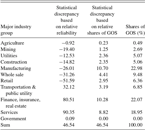
Table 8illustrates these two distributions by major industry sectors using 1997 data. The aggregate discrepancy for 1997 was 46.5 billion dollars, that is, GDI was 46.5 billion dollars below GDP. Under the approach based on industry profit shares, the discrepancy was distributed to each sector as an increase in its initial VA estimates in the GDP-by-industry accounts in column 3, proportional to its share of total GOS in column 4. By contrast, GLS estimation, based on relative reliability of initial estimates in both IO and GDP-by-industry accounts, resulted in
Table 8. Comparison of distributions of the aggregate statistical discrepancy by major sector (in billions of dollars)
Statistical Statistical discrepancy discrepancy
based based
Major industry on relative on relative Shares of group reliability shares of GOS GOS (%)
Agriculture −0.92 0.23 0.49 Mining −19.40 1.25 2.69 Utilities −12.53 2.36 5.07 Construction −14.82 2.35 5.06 Manufacturing −26.01 10.70 22.98 Whole sale −31.26 4.41 9.48 Retail −51.59 2.95 6.36 Transportation &
NOTE: GOS, gross operating surplus measuring industry profits, is one of the three com-ponents of VA estimates compiled by the GDP-by-industry accounts. Estimate of statistical discrepancy distributed to each sector is measured as the change, as a result of reconciliation, in that sector’s initial VA estimates in the GDP-by-industry accounts.
either positive or negative adjustments to the sectors’ initial VA estimates in column 2.
Balanced results from the GLS approach should improve the credibility of further data derived from the balanced estimates. For example, estimates of intermediate input data are used by BEA to compile annual industry KLEMS (capital, labor, energy, materials, and services) data and by the Federal Reserve Board to produce industry productivity indexes. Balanced estimates of intermediate inputs represent more accurate allocations of intermediate inputs across industries, and, hence, should help improve the accuracy of industry KLEMS data and productivity data compiled from them.
The degree of impact on data derived from balanced esti-mates may vary. For example, BLS produces industry output and employment projections using estimates of gross output from annual IO accounts at BEA. Because initial estimates of gross output are considered reliable, using balanced estimates of gross output should not substantially affect industry output projections. However, because initial VA estimates are less re-liable, the impact should be greater on statistics compiled using balanced estimates of VA.
6. CONCLUSION
The study demonstrates the empirical feasibility and compu-tational efficiency of using a GLS method to reconcile a large disaggregated system of accounts according to estimated rela-tive reliabilities of initial data. GLS reconciled estimates offer convincing economic interpretations and enhance the accuracy and credibility of estimates in national accounts. The GLS es-timates of industry statistical discrepancies trace the aggregate discrepancy to its sources.
This article makes a first attempt to systematically collect available objective information on the reliability of initial data and to use this information to reconcile the U.S. system of industry accounts. In this study, however, initial estimates of final expenditures were considered final and were not adjusted. This is an assumption not supported by statistical evidence. Thus, a future extension of this study will relax this restriction and will allow all initial data to be adjusted.
210 Journal of Business & Economic Statistics, April 2012
APPENDIX: NAICS INDUSTRY CODES AND INDUSTRY DESCRIPTION
Industry Industry description Industry Industry description
111CA Farms 486 Pipeline transportation
113FF Forestry, fishing, and related activities 487OS Other transportation and support activities 211 Oil and gas extraction 493 Warehousing and storage
212 Mining, except oil and gas 511 Publishing industries (includes software) 213 Support activities for mining 512 Motion picture and sound recording industries 22 Utilities 513 Broadcasting and telecommunications 23 Construction 514 Information and data processing services
311FT Food and beverage and tobacco products 521CI Federal Reserve banks, credit intermediation, and related activities 313TT Textile mills and textile product mills 523 Securities, commodity contracts, and investments
315AL Apparel and leather and allied products 524 Insurance carriers and related activities 321 Wood products 525 Funds, trusts, and other financial vehicles 322 Paper products 531 Real estate
323 Printing and related support activities 532RL Rental and leasing services and lessors of intangible assets 324 Petroleum and coal products 5411 Legal services
325 Chemical products 5412OP Miscellaneous professional, scientific and technical services 326 Plastics and rubber products 5415 Computer systems design and related services
327 Nonmetallic mineral products 55 Management of companies and enterprises 331 Primary metals 561 Administrative and support services 332 Fabricated metal products 562 Waste management and remediation services 333 Machinery 61 Educational services
334 Computer and electronic products 621 Ambulatory health care services
335 Electrical equipment, appliances, and components 622HO Hospitals and nursing and residential care facilities 3361MV Motor vehicles, bodies and trailers, and parts 624 Social assistance
3364OT Other transportation equipment 711AS Performing arts, spectator sports, museums, and related activities 337 Furniture and related products 713 Amusements, gambling, and recreation industries
339 Miscellaneous manufacturing 721 Accommodation
42 Wholesale trade 722 Food services and drinking places 44RT Retail trade 81 Other services, except government 481 Air transportation GFE Federal government enterprises 482 Rail transportation GFG Federal general government
483 Water transportation GSLE State and local government enterprises 484 Truck transportation GSLG State and local general government 485 Transit and ground passenger transportation
ACKNOWLEDGMENTS
The author thanks three anonymous referees, Dale Jorgen-son, Williams Nordhaus, Peter Zadrozny, Tarek M. Harchaoui, and participants at the 2006 NBER-CIRW (National Bureau of Economic Research/Conference on Research in Income and Wealth) summer workshop and at the 2007 International Con-ference on Measurement Errors for their helpful comments and suggestions. The author thanks Zhi Wang for his input in the early stage of the project. This article represents the author’s views and does not necessarily represent official positions of the Bureau of Economic Analysis.
[Received April 2008. Revised February 2012.]
REFERENCES
ASR Analytics. (2005), “Study and Evaluation of Bureau of Economic Analysis National Income and Product Accounts Income Measures,” unpublished
report, Potomac, MD: ASR Analysis LLC. [203]
Bacharach, M. (1965), “Estimating Nonnegative Matrices From Marginal Data,” International Economic Review, 6, 294–310. [202,208]
Barker, T., van der Ploeg, F., and Weale, M. (1984), “A Balanced System of
National Accounts for the United Kingdom,”Review of Income and Wealth,
30(4), 461–485. [202,205]
Bartholdy, K. (1991), “A Generalization of the Friedlander Algorithm for
Bal-ancing of National Accounts Matrices,”Computer Science in Economics
and Management, 4, 165–174. [202]
Beaulieu, J. J., and Bartelsman, E. J. (2004), “Integrating Expenditure and Income Data: What to Do With the Statistical Discrepancy?” unpublished paper, Board of Governors of the Federal Reserve System. [202,203,208] Byron, R. P. (1978), “The Estimation of Large Social Account Matrices,”
Jour-nal of Royal Statistics,Series A, 141(3), 359–367. [202]
——— (1996), “Diagnostic Testing and Sensitivity Analysis in the Construc-tion of Social Accounting Matrices,”Journal of the Royal Statistical Society, Series A, 159(1), 133–148. [203]
Chen, B. (2006), “A Balanced System of Industry Accounts and Structural Distribution of Aggregate Statistical Discrepancy,” Working paper WP2006-8, Bureau of Economic Analysis, Washington, DC. [204,206,206]
Dagum, E. B., and Cholette, A. P. (2006),Benchmark, Temporal Distribution,
and Reconciliation Methods for Time Series, Lecture Notes in Statistics (Vol. 186), Berlin, Germany: Springer. [202,204]
Deming, W. E., and Stephan, D. F. (1940), “On the Least Squares Adjustment of a Sampled Frequency Table When the Expected Marginal Totals are Known,”Annuals of Mathematical Statistics, 11, 427–444. [202,208] Fixler, J. D., and Grimm, T. B. (2005), “Reliability of the NIPA
Esti-mates of U.S. Economic Activity,”Survey of Current Business, 85(2),
8–18. [204]
Stone, J. R. N. (1984), “Balancing the National Accounts: The Adjustment
of Initial Estimates—A Neglected Stage in Measurement,” in Demand
Equilibrium and Trade (Essays in Honor of Ivor F. Pearce), eds. A.
Ingham and A. M. Ulph, London: Macmillan. [202]
Stone, R., Meade, J. E., and Champernowne, D. G. (1942), “The Precision of
National Income Estimates,”Review of Economic Studies, 9(2), 111–125.
[202,205]
van der Ploeg, F. (1982a), “Reliability and the Adjustment of Sequences of
Large Systems and Tables of National Accounting Matrices,”Journal of
Royal Statistical Society,Series A, 145(2), 169–194. [202]
——— (1982b), “Generalized Least Square Methods for Balancing Large Sys-tems and Tables of National Accounts,”Review of Public Data Use, 12(1), 17–33. [202]
——— (1988), “Balancing Large Systems of National Accounts,”Computer
Science in Economics and Management, 1, 31–39. [202]
Weale, M. (1992), “Estimation of Data Measured With Error and Subject
to Linear Restrictions,” Journal of Applied Econometrics, 7(2), 167–
174. [202]