ISO/IEC JTC 1/SC 29/WG 1
N 2412
Date: 2005-12-03
ISO/IEC JTC 1/SC 29/WG 1 (ITU-T SG 16)
Coding of Still Pictures
JBIG
JPEG
Joint Bi-level Image Joint Photographic
Experts Group Experts Group
TITLE:
The JPEG-2000 Still Image Compression Standard
(Last Revised: 2005-12-03)
SOURCE:
Michael D. Adams
Assistant Professor
Dept. of Electrical and Computer Engineering
University of Victoria
P. O. Box 3055 STN CSC, Victoria, BC, V8W 3P6, CANADA
E-mail:
[email protected]
Web:
www.ece.uvic.ca/˜mdadams
PROJECT:
JPEG 2000
STATUS:
REQUESTED ACTION:
None
DISTRIBUTION:
Public
Contact:
ISO/IEC JTC 1/SC 29/WG 1 Convener—Dr. Daniel T. Lee
Yahoo! Asia, Sunning Plaza, Rm 2802, 10 Hysan Avenue, Causeway Bay, Hong Kong Yahoo! Inc, 701 First Avenue, Sunnyvale, California 94089, USA
The JPEG-2000 Still Image Compression Standard
∗
(Last Revised: 2005-12-03)
Michael D. Adams
Dept. of Electrical and Computer Engineering, University of Victoria
P. O. Box 3055 STN CSC, Victoria, BC, V8W 3P6, CANADA
E-mail:
[email protected]
Web:
www.ece.uvic.ca/˜mdadams
Abstract—JPEG 2000, a new international standard for still image com-pression, is discussed at length. A high-level introduction to the JPEG-2000 standard is given, followed by a detailed technical description of the JPEG-2000 Part-1 codec.
Keywords—JPEG 2000, still image compression/coding, standards.
I. INTRODUCTION
D
IGITAL IMAGERY is pervasive in our world today. Con-sequently, standards for the efficient representation and interchange of digital images are essential. To date, some of the most successful still image compression standards have re-sulted from the ongoing work of the Joint Photographic Experts Group (JPEG). This group operates under the auspices of Joint Technical Committee 1, Subcommittee 29, Working Group 1 (JTC 1/SC 29/WG 1), a collaborative effort between the In-ternational Organization for Standardization (ISO) and Interna-tional Telecommunication Union Standardization Sector (ITU-T). Both the JPEG [1–3] and JPEG-LS [4–6] standards were born from the work of the JPEG committee. For the last few years, the JPEG committee has been working towards the estab-lishment of a new standard known as JPEG 2000 (i.e., ISO/IEC 15444). The fruits of these labors are now coming to bear, as several parts of this multipart standard have recently been rati-fied including JPEG-2000 Part 1 (i.e., ISO/IEC 15444-1 [7]).In this paper, we provide a detailed technical description of the JPEG-2000 Part-1 codec, in addition to a brief overview of the JPEG-2000 standard. This exposition is intended to serve as a reader-friendly starting point for those interested in learning about JPEG 2000. Although many details are included in our presentation, some details are necessarily omitted. The reader should, therefore, refer to the standard [7] before attempting an implementation. The JPEG-2000 codec realization in the JasPer software [8–10] (developed by the author of this paper) may also serve as a practical guide for implementors. (See Ap-pendix A for more information about JasPer.) The reader may also find [11–13] to be useful sources of information on the JPEG-2000 standard.
The remainder of this paper is structured as follows. Sec-tion II begins with a overview of the JPEG-2000 standard. This is followed, in Section III, by a detailed description of the JPEG-2000 Part-1 codec. Finally, we conclude with some closing
re-∗This document is a revised version of the JPEG-2000 tutorial that I wrote
which appeared in the JPEG working group document WG1N1734. The original tutorial contained numerous inaccuracies, some of which were introduced by changes in the evolving draft standard while others were due to typographical errors. Hopefully, most of these inaccuracies have been corrected in this revised document. In any case, this document will probably continue to evolve over time. Subsequent versions of this document will be made available from my home page (the URL for which is provided with my contact information).
marks in Section IV. Throughout our presentation, a basic un-derstanding of image coding is assumed.
II. JPEG 2000
The JPEG-2000 standard supports lossy and lossless com-pression of single-component (e.g., grayscale) and multi-component (e.g., color) imagery. In addition to this basic com-pression functionality, however, numerous other features are provided, including: 1) progressive recovery of an image by fi-delity or resolution; 2) region of interest coding, whereby differ-ent parts of an image can be coded with differing fidelity; 3) ran-dom access to particular regions of an image without needing to decode the entire code stream; 4) a flexible file format with pro-visions for specifying opacity information and image sequences; and 5) good error resilience. Due to its excellent coding per-formance and many attractive features, JPEG 2000 has a very large potential application base. Some possible application ar-eas include: image archiving, Internet, web browsing, document imaging, digital photography, medical imaging, remote sensing, and desktop publishing.
A. Why JPEG 2000?
Work on the JPEG-2000 standard commenced with an initial call for contributions [14] in March 1997. The purpose of having a new standard was twofold. First, it would address a number of weaknesses in the existing JPEG standard. Second, it would provide a number of new features not available in the JPEG stan-dard. The preceding points led to several key objectives for the new standard, namely that it should: 1) allow efficient lossy and lossless compression within a single unified coding framework, 2) provide superior image quality, both objectively and subjec-tively, at low bit rates, 3) support additional features such as rate and resolution scalability, region of interest coding, and a more flexible file format, 4) avoid excessive computational and mem-ory complexity. Undoubtedly, much of the success of the orig-inal JPEG standard can be attributed to its royalty-free nature. Consequently, considerable effort has been made to ensure that a minimally-compliant JPEG-2000 codec can be implemented free of royalties1.
B. Structure of the Standard
The JPEG-2000 standard is comprised of numerous parts, with the parts listed in Table I being defined at the time of this writing. For convenience, we will refer to the codec defined in
1Whether these efforts ultimately prove successful remains to be seen,
Part 1 (i.e., [7]) of the standard as the baseline codec. The base-line codec is simply the core (or minimal functionality) JPEG-2000 coding system. Part 2 (i.e., [15]) describes extensions to the baseline codec that are useful for certain “niche” applica-tions, while Part 3 (i.e., [16]) defines extensions for intraframe-style video compression. Part 5 (i.e., [17]) provides two refer-ence software implementations of the Part-1 codec, and Part 4 (i.e., [18]) provides a methodology for testing implementations for compliance with the standard. In this paper, we will, for the most part, limit our discussion to the baseline codec. Some of the extensions included in Part 2 will also be discussed briefly. Unless otherwise indicated, our exposition considers only the baseline system.
For the most part, the JPEG-2000 standard is written from the point of view of the decoder. That is, the decoder is defined quite precisely with many details being normative in nature (i.e., re-quired for compliance), while many parts of the encoder are less rigidly specified. Obviously, implementors must make a very clear distinction between normative and informative clauses in the standard. For the purposes of our discussion, however, we will only make such distinctions when absolutely necessary.
III. JPEG-2000 CODEC
Having briefly introduced the JPEG-2000 standard, we are now in a position to begin examining the JPEG-2000 codec in detail. The codec is based on wavelet/subband coding tech-niques [21, 22]. It handles both lossy and lossless compres-sion using the same transform-based framework, and borrows heavily on ideas from the embedded block coding with opti-mized truncation (EBCOT) scheme [23–25]. In order to fa-cilitate both lossy and lossless coding in an efficient manner, reversible integer-to-integer [26–28] and nonreversible real-to-real transforms are employed. To code transform data, the codec makes use of bit-plane coding techniques. For entropy coding, a context-based adaptive binary arithmetic coder [29] is used— more specifically, the MQ coder from the JBIG2 standard [30]. Two levels of syntax are employed to represent the coded image: a code stream and file format syntax. The code stream syntax is similar in spirit to that used in the JPEG standard.
The remainder of Section III is structured as follows. First, Sections III-A to III-C, discuss the source image model and how an image is internally represented by the codec. Next, Sec-tion III-D examines the basic structure of the codec. This is followed, in Sections III-E to III-M by a detailed explanation of the coding engine itself. Next, Sections III-N and III-O explain the syntax used to represent a coded image. Finally, Section III-P briefly describes some of the extensions included in III-Part 2 of the standard.
A. Source Image Model
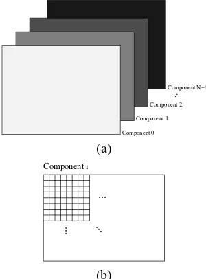
Before examining the internals of the codec, it is important to understand the image model that it employs. From the codec’s point of view, an image is comprised of one or more compo-nents (up to a limit of 214), as shown in Fig. 1(a). As illustrated
in Fig. 1(b), each component consists of a rectangular array of samples. The sample values for each component are integer val-ued, and can be either signed or unsigned with a precision from
Component 1 Component 2
...
Component 0
Component N−1
(a) Component i
...
...
...
(b)
Fig. 1. Source image model. (a) An image withNcomponents. (b) Individual component.
1 to 38 bits/sample. The signedness and precision of the sample data are specified on a per-component basis.
All of the components are associated with the same spatial ex-tent in the source image, but represent different spectral or aux-iliary information. For example, a RGB color image has three components with one component representing each of the red, green, and blue color planes. In the simple case of a grayscale image, there is only one component, corresponding to the lu-minance plane. The various components of an image need not be sampled at the same resolution. Consequently, the compo-nents themselves can have different sizes. For example, when color images are represented in a luminance-chrominance color space, the luminance information is often more finely sampled than the chrominance data.
B. Reference Grid
Given an image, the codec describes the geometry of the var-ious components in terms of a rectangular grid called the ref-erence grid. The refref-erence grid has the general form shown in Fig. 2. The grid is of size Xsiz×Ysiz with the origin lo-cated at its top-left corner. The region with its top-left corner at
(XOsiz,YOsiz)and bottom-right corner at(Xsiz−1,Ysiz−1)
is called the image area, and corresponds to the picture data to be represented. The width and height of the reference grid can-not exceed 232−1 units, imposing an upper bound on the size of an image that can be handled by the codec.
con-TABLE I PARTS OF THE STANDARD
Part Title Purpose Document
1 Core coding system Specifi es the core (or minimal functionality) JPEG-2000 codec. [7]
2 Extensions Specifi es additional functionalities that are useful in some applications but need not be supported by all codecs.
[15]
3 Motion JPEG 2000 Specifi es extensions to JPEG-2000 for intraframe-style video compression. [16] 4 Conformance testing Specifi es the procedure to be employed for compliance testing. [18] 5 Reference software Provides sample software implementations of the standard to serve as a guide for implementors. [17]
6 Compound image fi le format Defi nes a fi le format for compound documents. [19]
8 Secure JPEG 2000 Defi nes mechanisms for conditional access, integrity/authentication, and intellectual property rights protection.
∗
9 Interactivity tools, APIs and pro-tocols
Specifi es a client-server protocol for effi ciently communicating JPEG-2000 image data over net-works.
∗
10 3D and floating-point data Provides extensions for handling 3D (e.g., volumetric) and floating-point data. ∗
11 Wireless Provides channel coding and error protection tools for wireless applications. ∗
12 ISO base media fi le format Defi nes a common media fi le format used by Motion JPEG 2000 and MPEG 4. [20]
13 Entry-level JPEG 2000 encoder Specifi es an entry-level JPEG-2000 encoder. ∗
∗This part of the standard is still under development at the time of this writing.
(Xsiz−1,Ysiz−1) (XOsiz,YOsiz)
Xsiz−XOsiz Image Area (0,0)
Xsiz
Ysiz−YOsiz Ysiz
XOsiz
YOsiz
Fig. 2. Reference grid.
stitute samples of the component in question. Thus, in terms of its own coordinate system, a component will have the size
Xsiz XRsiz
−XOsiz XRsiz
× Ysiz
YRsiz
−YOsiz YRsiz
and its top-left sam-ple will correspond to the point XOsiz
XRsiz
,YOsiz YRsiz
.Note that the reference grid also imposes a particular alignment of sam-ples from the various components relative to one another.
From the diagram, the size of the image area is (Xsiz−
XOsiz)×(Ysiz−YOsiz). For a given image, many combina-tions of the Xsiz, Ysiz, XOsiz, and YOsiz parameters can be chosen to obtain an image area with the same size. Thus, one might wonder why the XOsiz and YOsiz parameters are not fixed at zero while the Xsiz and Ysiz parameters are set to the size of the image. As it turns out, there are subtle implications to changing the XOsiz and YOsiz parameters (while keeping the size of the image area constant). Such changes affect codec be-havior in several important ways, as will be described later. This behavior allows a number of basic operations to be performed more efficiently on coded images, such as cropping, horizon-tal/vertical flipping, and rotation by an integer multiple of 90 degrees.
C. Tiling
In some situations, an image may be quite large in compar-ison to the amount of memory available to the codec. Conse-quently, it is not always feasible to code the entire image as a
T7
T0 T1 T2
T3 T4 T5
T6 T8
(XOsiz,YOsiz) (0,0)
(XTOsiz,YTOsiz)
XTOsiz XTsiz XTsiz XTsiz
YTsiz YTsiz YTsiz YTOsiz
Ysiz
Xsiz
Fig. 3. Tiling on the reference grid.
single atomic unit. To solve this problem, the codec allows an image to be broken into smaller pieces, each of which is inde-pendently coded. More specifically, an image is partitioned into one or more disjoint rectangular regions called tiles. As shown in Fig. 3, this partitioning is performed with respect to the ref-erence grid by overlaying the refref-erence grid with a rectangu-lar tiling grid having horizontal and vertical spacings of XTsiz and YTsiz, respectively. The origin of the tiling grid is aligned with the point(XTOsiz,YTOsiz). Tiles have a nominal size of XTsiz×YTsiz, but those bordering on the edges of the image area may have a size which differs from the nominal size. The tiles are numbered in raster scan order (starting at zero).
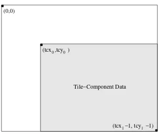
By mapping the position of each tile from the reference grid to the coordinate systems of the individual components, a par-titioning of the components themselves is obtained. For exam-ple, suppose that a tile has an upper left corner and lower right corner with coordinates(tx0,ty0)and(tx1−1,ty1−1),
respec-tcx0tcy0
Fig. 4. Tile-component coordinate system.
tively, where
(tcx0,tcy0) = (⌈tx0/XRsiz⌉,⌈ty0/YRsiz⌉) (1a)
(tcx1,tcy1) = (⌈tx1/XRsiz⌉,⌈ty1/YRsiz⌉). (1b)
These equations correspond to the illustration in Fig. 4. The por-tion of a component that corresponds to a single tile is referred to as a tile-component. Although the tiling grid is regular with respect to the reference grid, it is important to note that the grid may not necessarily be regular with respect to the coordinate systems of the components.
D. Codec Structure
The general structure of the codec is shown in Fig. 5 with the form of the encoder given by Fig. 5(a) and the decoder given by Fig. 5(b). From these diagrams, the key processes associated with the codec can be identified: 1) preprocess-ing/postprocessing, 2) intercomponent transform, 3) intracom-ponent transform, 4) quantization/dequantization, 5) tier-1 cod-ing, 6) tier-2 codcod-ing, and 7) rate control. The decoder structure essentially mirrors that of the encoder. That is, with the excep-tion of rate control, there is a one-to-one correspondence be-tween functional blocks in the encoder and decoder. Each func-tional block in the decoder either exactly or approximately in-verts the effects of its corresponding block in the encoder. Since tiles are coded independently of one another, the input image is (conceptually, at least) processed one tile at a time. In the sections that follow, each of the above processes is examined in more detail.
E. Preprocessing/Postprocessing
The codec expects its input sample data to have a nominal dynamic range that is approximately centered about zero. The preprocessing stage of the encoder simply ensures that this ex-pectation is met. Suppose that a particular component has P
bits/sample. The samples may be either signed or unsigned, leading to a nominal dynamic range of [−2P−1,2P−1−1] or
[0,2P−1], respectively. If the sample values are unsigned, the nominal dynamic range is clearly not centered about zero. Thus, the nominal dynamic range of the samples is adjusted by sub-tracting a bias of 2P−1from each of the sample values. If the
sample values for a component are signed, the nominal dynamic range is already centered about zero, and no processing is re-quired. By ensuring that the nominal dynamic range is centered
about zero, a number of simplifying assumptions could be made in the design of the codec (e.g., with respect to context model-ing, numerical overflow, etc.).
The postprocessing stage of the decoder essentially undoes the effects of preprocessing in the encoder. If the sample val-ues for a component are unsigned, the original nominal dynamic range is restored. Lastly, in the case of lossy coding, clipping is performed to ensure that the sample values do not exceed the allowable range.
F. Intercomponent Transform
In the encoder, the preprocessing stage is followed by the for-ward intercomponent transform stage. Here, an intercomponent transform can be applied to the tile-component data. Such a transform operates on all of the components together, and serves to reduce the correlation between components, leading to im-proved coding efficiency.
Only two intercomponent transforms are defined in the base-line JPEG-2000 codec: the irreversible color transform (ICT) and reversible color transform (RCT). The ICT is nonreversible and real-to-real in nature, while the RCT is reversible and integer-to-integer. Both of these transforms essentially map im-age data from the RGB to YCrCb color space. The transforms are defined to operate on the first three components of an image, with the assumption that components 0, 1, and 2 correspond to the red, green, and blue color planes. Due to the nature of these transforms, the components on which they operate must be sampled at the same resolution (i.e., have the same size). As a consequence of the above facts, the ICT and RCT can only be employed when the image being coded has at least three com-ponents, and the first three components are sampled at the same resolution. The ICT may only be used in the case of lossy cod-ing, while the RCT can be used in either the lossy or lossless case. Even if a transform can be legally employed, it is not necessary to do so. That is, the decision to use a multicompo-nent transform is left at the discretion of the encoder. After the intercomponent transform stage in the encoder, data from each component is treated independently.
The ICT is nothing more than the classic RGB to YCrCb color space transform. The forward transform is defined as
corresponding to the red, green, and blue color planes, respec-tively, andV0(x,y),V1(x,y), andV2(x,y)are the output
compo-nents corresponding to the Y, Cr, and Cb planes, respectively. The inverse transform can be shown to be
Preprocessing
Quantization Tier−1Encoder Tier−2Encoder
Coded
Fig. 5. Codec structure. The structure of the (a) encoder and (b) decoder.
transform is given by
are defined as above. The inverse transform can be shown to be
U1(x,y) =V0(x,y)−41(V1(x,y) +V2(x,y)) (5a)
U0(x,y) =V2(x,y) +U1(x,y) (5b)
U2(x,y) =V1(x,y) +U1(x,y) (5c)
The inverse intercomponent transform stage in the decoder essentially undoes the effects of the forward intercomponent transform stage in the encoder. If a multicomponent transform was applied during encoding, its inverse is applied here. Unless the transform is reversible, however, the inversion may only be approximate due to the effects of finite-precision arithmetic.
G. Intracomponent Transform
Following the intercomponent transform stage in the encoder is the intracomponent transform stage. In this stage, transforms that operate on individual components can be applied. The par-ticular type of operator employed for this purpose is the wavelet transform. Through the application of the wavelet transform, a component is split into numerous frequency bands (i.e., sub-bands). Due to the statistical properties of these subband signals, the transformed data can usually be coded more efficiently than the original untransformed data.
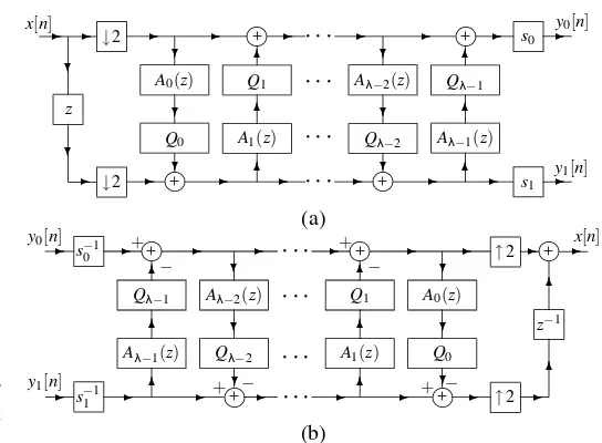
Both reversible integer-to-integer [26, 27, 31–33] and non-reversible real-to-real wavelet transforms are employed by the baseline codec. The basic building block for such transforms is the 1-D 2-channel perfect-reconstruction (PR) uniformly-maximally-decimated (UMD) filter bank (FB) which has the general form shown in Fig. 6. Here, we focus on the lifting realization of the UMDFB [34, 35], as it can be used to imple-ment the reversible integer-to-integer and nonreversible real-to-real wavelet transforms employed by the baseline codec. In fact,
❤
Fig. 6. Lifting realization of a 1-D 2-channel PR UMDFB. (a) Analysis side. (b) Synthesis side.
for this reason, it is likely that this realization strategy will be employed by many codec implementations. The analysis side of the UMDFB, depicted in Fig. 6(a), is associated with the for-ward transform, while the synthesis side, depicted in Fig. 6(b), is associated with the inverse transform. In the diagram, the
{Ai(z)}iλ=−01,{Qi(x)} λ−1
i=0, and{si} 1
i=0denote filter transfer
func-tions, quantization operators, and (scalar) gains, respectively. To obtain integer-to-integer mappings, the{Qi(x)}λi=−01are selected
such that they always yield integer values, and the{si}1i=0are
chosen as integers. For real-to-real mappings, the{Qi(x)}λi=−01
are simply chosen as the identity, and the{si}1i=0 are selected
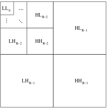
LL0 ployed. To compute the forward transform, we apply the anal-ysis side of the 2-D UMDFB to the tile-component data in an iterative manner, resulting in a number of subband signals be-ing produced. Each application of the analysis side of the 2-D UMDFB yields four subbands: 1) horizontally and vertically lowpass (LL), 2) horizontally lowpass and vertically highpass (LH), 3) horizontally highpass and vertically lowpass (HL), and 4) horizontally and vertically highpass (HH). A (R−1)-level wavelet decomposition is associated with R resolution levels, numbered from 0 to R−1, with 0 and R−1 corresponding to the coarsest and finest resolutions, respectively. Each sub-band of the decomposition is identified by its orientation (e.g., LL, LH, HL, HH) and its corresponding resolution level (e.g., 0,1, . . . ,R−1). The input tile-component signal is considered to be the LLR−1band. At each resolution level (except the lowest)
the LL band is further decomposed. For example, the LLR−1
band is decomposed to yield the LLR−2, LHR−2, HLR−2, and
HHR−2 bands. Then, at the next level, the LLR−2band is
de-composed, and so on. This process repeats until the LL0band
is obtained, and results in the subband structure illustrated in Fig. 7. In the degenerate case where no transform is applied,
R=1, and we effectively have only one subband (i.e., theLL0
band).
As described above, the wavelet decomposition can be as-sociated with data atRdifferent resolutions. Suppose that the top-left and bottom-right samples of a tile-component have co-ordinates(tcx0,tcy0)and(tcx1−1,tcy1−1), respectively. This
being the case, the top-left and bottom-right samples of the tile-component at resolutionrhave coordinates(trx0,try0)and
(trx1−1,try1−1), respectively, given by
where ris the particular resolution of interest. Thus, the tile-component signal at a particular resolution has the size(trx1−
trx0)×(try1−try0).
Not only are the coordinate systems of the resolution levels important, but so too are the coordinate systems for the various
subbands. Suppose that we denote the coordinates of the upper left and lower right samples in a subband as (tbx0,tby0) and
whereris the resolution level to which the band belongs,Ris the number of resolution levels, and tcx0, tcy0, tcx1, and tcy1are
as defined in (1). Thus, a particular band has the size(tbx1−
tbx0)×(tby1−tby0). From the above equations, we can also
see that(tbx0,tby0) = (trx0,try0)and(tbx1,tby1) = (trx1,try1)
for theLLrband, as one would expect. (This should be the case
since theLLrband is equivalent to a reduced resolution version
of the original data.) As will be seen, the coordinate systems for the various resolutions and subbands of a tile-component play an important role in codec behavior.
By examining (1), (6), and (7), we observe that the coordi-nates of the top-left sample for a particular subband, denoted
(tbx0,tby0), are partially determined by the XOsiz and YOsiz
parameters of the reference grid. At each level of the decompo-sition, the parity (i.e., oddness/evenness) of tbx0and tby0affects
the outcome of the downsampling process (since downsampling is shift variant). In this way, the XOsiz and YOsiz parameters have a subtle, yet important, effect on the transform calculation. Having described the general transform framework, we now describe the two specific wavelet transforms supported by the baseline codec: the 5/3 and 9/7 transforms. The 5/3 transform is reversible, integer-to-integer, and nonlinear. This transform was proposed in [26], and is simply an approximation to a linear wavelet transform proposed in [39]. The 5/3 transform has an underlying 1-D UMDFB with the parameters:
λ=2, A0(z) =−12(z+1), A1(z) =14(1+z−1), (8)
Q0(x) =− ⌊−x⌋, Q1(x) =
x+12
, s0=s1=1.
pa-rameters:
λ=4, A0(z) =α0(z+1), A1(z) =α1(1+z−1), (9)
A2(z) =α2(z+1), A3(z) =α3(1+z−1),
Qi(x) =x fori=0,1,2,3,
α0≈ −1.586134, α1≈ −0.052980, α2≈0.882911,
α3≈0.443506, s0≈1/1.230174, s1=−1/s0.
Since the 5/3 transform is reversible, it can be employed for either lossy or lossless coding. The 9/7 transform, lacking the reversible property, can only be used for lossy coding. The num-ber of resolution levels is a parameter of each transform. A typi-cal value for this parameter is six (for a sufficiently large image). The encoder may transform all, none, or a subset of the compo-nents. This choice is at the encoder’s discretion.
The inverse intracomponent transform stage in the decoder essentially undoes the effects of the forward intracomponent transform stage in the encoder. If a transform was applied to a particular component during encoding, the corresponding in-verse transform is applied here. Due to the effects of finite-precision arithmetic, the inversion process is not guaranteed to be exact unless reversible transforms are employed.
H. Quantization/Dequantization
In the encoder, after the tile-component data has been trans-formed (by intercomponent and/or intracomponent transforms), the resulting coefficients are quantized. Quantization allows greater compression to be achieved, by representing transform coefficients with only the minimal precision required to obtain the desired level of image quality. Quantization of transform co-efficients is one of the two primary sources of information loss in the coding path (the other source being the discarding of cod-ing pass data as will be described later).
Transform coefficients are quantized using scalar quantiza-tion with a deadzone. A different quantizer is employed for the coefficients of each subband, and each quantizer has only one parameter, its step size. Mathematically, the quantization pro-cess is defined as
V(x,y) =⌊|U(x,y)|/∆⌋sgnU(x,y) (10) where ∆ is the quantizer step size, U(x,y) is the input sub-band signal, andV(x,y)denotes the output quantizer indices for the subband. Since this equation is specified in an informative clause of the standard, encoders need not use this precise for-mula. This said, however, it is likely that many encoders will, in fact, use the above equation.
The baseline codec has two distinct modes of operation, re-ferred to herein as integer mode and real mode. In integer mode, all transforms employed are integer-to-integer in nature (e.g., RCT, 5/3 WT). In real mode, real-to-real transforms are em-ployed (e.g., ICT, 9/7 WT). In integer mode, the quantizer step sizes are always fixed at one, effectively bypassing quantization and forcing the quantizer indices and transform coefficients to be one and the same. In this case, lossy coding is still possible, but rate control is achieved by another mechanism (to be dis-cussed later). In the case of real mode (which implies lossy cod-ing), the quantizer step sizes are chosen in conjunction with rate
control. Numerous strategies are possible for the selection of the quantizer step sizes, as will be discussed later in Section III-L.
As one might expect, the quantizer step sizes used by the en-coder are conveyed to the deen-coder via the code stream. In pass-ing, we note that the step sizes specified in the code stream are relative and not absolute quantities. That is, the quantizer step size for each band is specified relative to the nominal dynamic range of the subband signal.
In the decoder, the dequantization stage tries to undo the ef-fects of quantization. This process, however, is not usually in-vertible, and therefore results in some information loss. The quantized transform coefficient values are obtained from the quantizer indices. Mathematically, the dequantization process is defined as
U(x,y) = (V(x,y) +rsgnV(x,y))∆ (11) where∆is the quantizer step size,ris a bias parameter,V(x,y)
are the input quantizer indices for the subband, andU(x,y)is the reconstructed subband signal. Although the value of r is not normatively specified in the standard, it is likely that many decoders will use the value of one half.
I. Tier-1 Coding
After quantization is performed in the encoder, tier-1 coding takes place. This is the first of two coding stages. The quantizer indices for each subband are partitioned into code blocks. Code blocks are rectangular in shape, and their nominal size is a free parameter of the coding process, subject to certain constraints, most notably: 1) the nominal width and height of a code block must be an integer power of two, and 2) the product of the nom-inal width and height cannot exceed 4096.
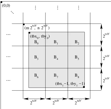
Suppose that the nominal code block size is tentatively cho-sen to be 2xcb×2ycb. In tier-2 coding, yet to be discussed, code blocks are grouped into what are called precincts. Since code blocks are not permitted to cross precinct boundaries, a re-duction in the nominal code block size may be required if the precinct size is sufficiently small. Suppose that the nominal code block size after any such adjustment is 2xcb’×2ycb’where
xcb’≤xcb and ycb’≤ycb. The subband is partitioned into code blocks by overlaying the subband with a rectangular grid having horizontal and vertical spacings of 2xcb’and 2ycb’, respectively, as shown in Fig. 8. The origin of this grid is anchored at(0,0)in the coordinate system of the subband. A typical choice for the nominal code block size is 64×64 (i.e., xcb=6 and ycb=6).
Let us, again, denote the coordinates of the top-left sample in a subband as(tbx0,tby0). As explained in Section III-G, the quantity(tbx0,tby0)is partially determined by the reference grid parameters XOsiz and YOsiz. In turn, the quantity(tbx0,tby0)
affects the position of code block boundaries within a subband. In this way, the XOsiz and YOsiz parameters have an impor-tant effect on the behavior of the tier-1 coding process (i.e., they affect the location of code block boundaries).
tbx0 tby0 ( , )
tbx1 tby1
( −1, −1)
B0 B2
B5
B4
B3
B1
B6 B7 B8
2xcb’
2xcb’ 2xcb’
2ycb’
2ycb’
2ycb’
2xcb’ 2ycb’
(m , n ) (0,0)
...
...
...
...
...
...
...
Fig. 8. Partitioning of a subband into code blocks.
process is, therefore, a collection of coding passes for the vari-ous code blocks.
On the decoder side, the bit-plane coding passes for the var-ious code blocks are input to the tier-1 decoder, these passes are decoded, and the resulting data is assembled into subbands. In this way, we obtain the reconstructed quantizer indices for each subband. In the case of lossy coding, the reconstructed quantizer indices may only be approximations to the quantizer indices originally available at the encoder. This is attributable to the fact that the code stream may only include a subset of the coding passes generated by the tier-1 encoding process. In the lossless case, the reconstructed quantizer indices must be same as the original indices on the encoder side, since all cod-ing passes must be included for lossless codcod-ing.
J. Bit-Plane Coding
The tier-1 coding process is essentially one of bit-plane cod-ing. After all of the subbands have been partitioned into code blocks, each of the resulting code blocks is independently coded using a bit-plane coder. Although the bit-plane coding tech-nique employed is similar to those used in the embedded ze-rotree wavelet (EZW) [41] and set partitioning in hierarchical trees (SPIHT) [42] codecs, there are two notable differences: 1) no interband dependencies are exploited, and 2) there are three coding passes per bit plane instead of two. The first dif-ference follows from the fact that each code block is completely contained within a single subband, and code blocks are coded in-dependently of one another. By not exploiting interband depen-dencies, improved error resilience can be achieved. The second difference is arguably less fundamental. Using three passes per bit plane instead of two reduces the amount of data associated with each coding pass, facilitating finer control over rate. Also, using an additional pass per bit plane allows better prioritization of important data, leading to improved coding efficiency.
As noted above, there are three coding passes per bit plane. In
order, these passes are as follows: 1) significance, 2) refinement, and 3) cleanup. All three types of coding passes scan the sam-ples of a code block in the same fixed order shown in Fig. 10. The code block is partitioned into horizontal stripes, each hav-ing a nominal height of four samples. If the code block height is not a multiple of four, the height of the bottom stripe will be less than this nominal value. As shown in the diagram, the stripes are scanned from top to bottom. Within a stripe, columns are scanned from left to right. Within a column, samples are scanned from top to bottom.
The bit-plane encoding process generates a sequence of sym-bols for each coding pass. Some or all of these symsym-bols may be entropy coded. For the purposes of entropy coding, a context-based adaptive binary arithmetic coder is used—more specifi-cally, the MQ coder from the JBIG2 standard [30]. For each pass, all of the symbols are either arithmetically coded or raw coded (i.e., the binary symbols are emitted as raw bits with sim-ple bit stuffing). The arithmetic and raw coding processes both ensure that certain bit patterns never occur in the output, allow-ing such patterns to be used for error resilience purposes.
Cleanup passes always employ arithmetic coding. In the case of the significance and refinement passes, two possibilities ex-ist, depending on whether the so called arithmetic-coding bypass mode (also known as lazy mode) is enabled. If lazy mode is en-abled, only the significance and refinement passes for the four most significant bit planes use arithmetic coding, while the re-maining such passes are raw coded. Otherwise, all significance and refinement passes are arithmetically coded. The lazy mode allows the computational complexity of bit-plane coding to be significantly reduced, by decreasing the number of symbols that must be arithmetically coded. This comes, of course, at the cost of reduced coding efficiency.
As indicated above, coding pass data can be encoded using one of two schemes (i.e., arithmetic or raw coding). Consecu-tive coding passes that employ the same encoding scheme con-stitute what is known as a segment. All of the coding passes in a segment can collectively form a single codeword or each coding pass can form a separate codeword. Which of these is the case is determined by the termination mode in effect. Two termina-tion modes are supported: per-pass terminatermina-tion and per-segment termination. In the first case, only the last coding pass of a seg-ment is terminated. In the second case, all coding passes are terminated. Terminating all coding passes facilitates improved error resilience at the expense of decreased coding efficiency.
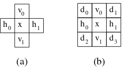
Since context-based arithmetic coding is employed, a means for context selection is necessary. Generally speaking, context selection is performed by examining state information for the 4-connected or 8-connected neighbors of a sample as shown in Fig. 9.
In our explanation of the coding passes that follows, we focus on the encoder side as this facilitates easier understanding. The decoder algorithms follow directly from those employed on the encoder side.
J.1 Significance Pass
h0
v0
h1
v1
x
(a)
h0
v0
d0
h1
d3
d1
d2 v1
x
(b)
Fig. 9. Templates for context selection. The (a) 4-connected and (b) 8-connected neighbors.
to be significant and are predicted to become significant during the processing of the current bit plane. The samples in the code block are scanned in the order shown previously in Fig. 10. If a sample has not yet been found to be significant, and is pre-dicted to become significant, the significance of the sample is coded with a single binary symbol. If the sample also happens to be significant, its sign is coded using a single binary sym-bol. In pseudocode form, the significance pass is described by Algorithm 1.
Algorithm 1Significance pass algorithm.
1: foreach sample in code blockdo
2: ifsample previously insignifi cantandpredicted to become signifi cant dur-ing current bit planethen
3: code signifi cance of sample /* 1 binary symbol */ 4: ifsample signifi cantthen
5: code sign of sample /* 1 binary symbol */ 6: endif
7: endif
8: endfor
If the most significant bit plane is being processed, all samples are predicted to remain insignificant. Otherwise, a sample is predicted to become significant if any 8-connected neighbor has already been found to be significant. As a consequence of this prediction policy, the significance and refinement passes for the most significant bit plane are always empty and not explicitly coded.
The symbols generated during the significance pass may or may not be arithmetically coded. If arithmetic coding is em-ployed, the binary symbol conveying significance information is coded using one of nine contexts. The particular context used is selected based on the significance of the sample’s 8-connected neighbors and the orientation of the subband with which the sample is associated (e.g., LL, LH, HL, HH). In the case that arithmetic coding is used, the sign of a sample is coded as the difference between the actual and predicted sign. Otherwise, the sign is coded directly. Sign prediction is performed using the significance and sign information for 4-connected neighbors.
J.2 Refinement Pass
The second coding pass for each bit plane is the refinement pass. This pass signals subsequent bits after the most significant bit for each sample. The samples of the code block are scanned using the order shown earlier in Fig. 10. If a sample was found to be significant in a previous bit plane, the next most significant bit of that sample is conveyed using a single binary symbol. This process is described in pseudocode form by Algorithm 2.
Like the significance pass, the symbols of the refinement pass may or may not be arithmetically coded. If arithmetic coding is
Algorithm 2Refinement pass algorithm.
1: foreach sample in code blockdo
2: ifsample found signifi cant in previous bit planethen
3: code next most signifi cant bit in sample /* 1 binary symbol */ 4: endif
5: endfor
...
...
...
...
...
Fig. 10. Sample scan order within a code block.
employed, each refinement symbol is coded using one of three contexts. The particular context employed is selected based on if the second MSB position is being refined and the significance of 8-connected neighbors.
J.3 Cleanup Pass
The third (and final) coding pass for each bit plane is the cleanup pass. This pass is used to convey significance and (as necessary) sign information for those samples that have not yet been found to be significant and are predicted to remain insignif-icant during the processing of the current bit plane.
Conceptually, the cleanup pass is not much different from the significance pass. The key difference is that the cleanup pass conveys information about samples that are predicted to remain insignificant, rather than those that are predicted to become sig-nificant. Algorithmically, however, there is one important differ-ence between the cleanup and significance passes. In the case of the cleanup pass, samples are sometimes processed in groups, rather than individually as with the significance pass.
Recall the scan pattern for samples in a code block, shown earlier in Fig. 10. A code block is partitioned into stripes with a nominal height of four samples. Then, stripes are scanned from top to bottom, and the columns within a stripe are scanned from left to right. For convenience, we will refer to each column within a stripe as a vertical scan. That is, each vertical arrow in the diagram corresponds to a so called vertical scan. As will soon become evident, the cleanup pass is best explained as op-erating on vertical scans (and not simply individual samples).
Algorithm 3Cleanup pass algorithm.
1: foreach vertical scan in code blockdo
2: iffour samples in vertical scanandall previously insignifi cant and unvisited
andnone have signifi cant 8-connected neighborthen
3: code number of leading insignifi cant samples via aggregation 4: skip over any samples indicated as insignifi cant by aggregation 5: endif
6: whilemore samples to process in vertical scando
7: ifsample previously insignifi cant and unvisitedthen
8: code signifi cance of sample if not already implied by run /* 1 binary symbol */
9: ifsample signifi cantthen
10: code sign of sample /* 1 binary symbol */ 11: endif
12: endif
13: endwhile
14: endfor
When aggregation mode is entered, the four samples of the vertical scan are examined. If all four samples are insignificant, an all-insignificant aggregation symbol is coded, and processing of the vertical scan is complete. Otherwise, a some-significant aggregation symbol is coded, and two binary symbols are then used to code the number of leading insignificant samples in the vertical scan.
The symbols generated during the cleanup pass are always arithmetically coded. In the aggregation mode, the aggregation symbol is coded using a single context, and the two symbol run length is coded using a single context with a fixed uniform prob-ability distribution. When aggregation mode is not employed, significance and sign coding function just as in the case of the significance pass.
K. Tier-2 Coding
In the encoder, tier-1 encoding is followed by tier-2 encoding. The input to the tier-2 encoding process is the set of bit-plane coding passes generated during tier-1 encoding. In tier-2 en-coding, the coding pass information is packaged into data units called packets, in a process referred to as packetization. The resulting packets are then output to the final code stream. The packetization process imposes a particular organization on cod-ing pass data in the output code stream. This organization facil-itates many of the desired codec features including rate scalabil-ity and progressive recovery by fidelscalabil-ity or resolution.
A packet is nothing more than a collection of coding pass data. Each packet is comprised of two parts: a header and body. The header indicates which coding passes are included in the packet, while the body contains the actual coding pass data it-self. In the code stream, the header and body may appear to-gether or separately, depending on the coding options in effect.
Rate scalability is achieved through (quality) layers. The coded data for each tile is organized into L layers, numbered from 0 toL−1, whereL≥1. Each coding pass is either assigned to one of theLlayers or discarded. The coding passes containing the most important data are included in the lower layers, while the coding passes associated with finer details are included in higher layers. During decoding, the reconstructed image quality improves incrementally with each successive layer processed. In the case of lossy compression, some coding passes may be dis-carded (i.e., not included in any layer) in which case rate control
must decide which passes to include in the final code stream. In the lossless case, all coding passes must be included. If multi-ple layers are employed (i.e.,L>1), rate control must decide in which layer each coding pass is to be included. Since some cod-ing passes may be discarded, tier-2 codcod-ing is the second primary source of information loss in the coding path.
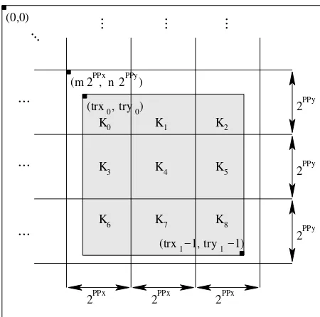
Recall, from Section III-I, that each coding pass is associated with a particular component, resolution level, subband, and code block. In tier-2 coding, one packet is generated for each com-ponent, resolution level, layer, and precinct 4-tuple. A packet need not contain any coding pass data at all. That is, a packet can be empty. Empty packets are sometimes necessary since a packet must be generated for every component-resolution-layer-precinct combination even if the resulting packet conveys no new information.
As mentioned briefly in Section III-G, a precinct is essen-tially a grouping of code blocks within a subband. The precinct partitioning for a particular subband is derived from a partition-ing of its parent LL band (i.e., the LL band at the next higher resolution level). Each resolution level has a nominal precinct size. The nominal width and height of a precinct must be a power of two, subject to certain constraints (e.g., the maximum width and height are both 215). The LL band associated with each resolution level is divided into precincts. This is accom-plished by overlaying the LL band with a regular grid having horizontal and vertical spacings of 2PPx and 2PPy, respectively, as shown in Fig. 11, where the grid is aligned with the origin of the LL band’s coordinate system. The precincts bordering on the edge of the subband may have dimensions smaller than the nominal size. Each of the resulting precinct regions is then mapped into its child subbands (if any) at the next lower resolu-tion level. This is accomplished by using the coordinate trans-formation(u,v) = (⌈x/2⌉,⌈y/2⌉)where(x,y)and(u,v)are the coordinates of a point in the LL band and child subband, re-spectively. Due to the manner in which the precinct partitioning is performed, precinct boundaries always align with code block boundaries. Some precincts may also be empty. Suppose the nominal code block size is 2xcb’×2ycb’. This results nominally
in 2PPx’−xcb’×2PPy’−ycb’ groups of code blocks in a precinct,
where
PPx’=
(
PPx forr=0
PPx−1 forr>0 (12)
PPy’=
(
PPy forr=0
PPy−1 forr>0 (13)
andris the resolution level.
Since coding pass data from different precincts are coded in separate packets, using smaller precincts reduces the amount of data contained in each packet. If less data is contained in a packet, a bit error is likely to result in less information loss (since, to some extent, bit errors in one packet do not affect the decoding of other packets). Thus, using a smaller precinct size leads to improved error resilience, while coding efficiency is de-graded due to the increased overhead of having a larger number of packets.
trx0 try0 ( , )
trx1 try1
( −1, −1)
K0 K2
K5
K4
K3
K1
K6 K7 K8
2PPx
2PPx 2PPx
2PPy
2PPy
2PPy
2PPx 2PPy
(m , n ) (0,0)
...
...
...
...
...
...
...
Fig. 11. Partitioning of a resolution into precincts.
are five builtin progressions defined: 1) layer-resolution-component-position ordering, 2) resolution-layer-component-position ordering, 3) resolution-resolution-layer-component-position-component-layer or-dering, 4) position-component-resolution-layer oror-dering, and 5) component-position-resolution-layer ordering. The sort order for the packets is given by the name of the ordering, where po-sition refers to precinct number, and the sorting keys are listed from most significant to least significant. For example, in the case of the first ordering given above, packets are ordered first by layer, second by resolution, third by component, and last by precinct. This corresponds to a progressive recovery by fi-delity scenario. The second ordering above is associated with progressive recovery by resolution. The three remaining order-ings are somewhat more esoteric. It is also possible to specify additional user-defined progressions at the expense of increased coding overhead.
In the simplest scenario, all of the packets from a particular tile appear together in the code stream. Provisions exist, how-ever, for interleaving packets from different tiles, allowing fur-ther flexibility on the ordering of data. If, for example, progres-sive recovery of a tiled image was desired, one would probably include all of the packets associated with the first layer of the various tiles, followed by those packets associated with the sec-ond layer, and so on.
In the decoder, the tier-2 decoding process extracts the various coding passes from the code stream (i.e., depacketization) and associates each coding pass with its corresponding code block. In the lossy case, not all of the coding passes are guaranteed to be present since some may have been discarded by the encoder. In the lossless case, all of the coding passes must be present in the code stream.
In the sections that follow, we describe the packet coding pro-cess in more detail. For ease of understanding, we choose to ex-plain this process from the point of view of the encoder. The de-coder algorithms, however, can be trivially deduced from those
...
Fig. 12. Code block scan order within a precinct.
of the encoder.
K.1 Packet Header Coding
The packet header corresponding to a particular component, resolution level, layer, and precinct, is encoded as follows. First, a single binary symbol is encoded to indicate if any coding pass data is included in the packet (i.e., if the packet is non-empty). If the packet is empty, no further processing is required and the algorithm terminates. Otherwise, we proceed to examine each subband in the resolution level in a fixed order. For each sub-band, we visit the code blocks belonging to the precinct of inter-est in raster scan order as shown in Fig. 12. To process a single code block, we begin by determining if any new coding pass data is to be included. If no coding pass data has yet been in-cluded for this code block, the inclusion information is conveyed via a quadtree-based coding procedure. Otherwise, a binary symbol is emitted indicating the presence or absence of new coding pass data for the code block. If no new coding passes are included, we proceed to the processing of the next code block in the precinct. Assuming that new coding pass data are to be included, we continue with our processing of the current code block. If this is the first time coding pass data have been cluded for the code block, we encode the number of leading in-significant bit planes for the code block using a quadtree-based coding algorithm. Then, the number of new coding passes, and the length of the data associated with these passes is encoded. A bit stuffing algorithm is applied to all packet header data to en-sure that certain bit patterns never occur in the output, allowing such patterns to be used for error resilience purposes. The entire packet header coding process is summarized by Algorithm 4.
Algorithm 4Packet header coding algorithm.
1: ifpacket not emptythen
2: code non-empty packet indicator /* 1 binary symbol */ 3: foreach subband in resolution leveldo
4: foreach code block in subband precinctdo
5: code inclusion information /* 1 binary symbol or tag tree */ 6: ifno new coding passes includedthen
7: skip to next code block 8: endif
9: iffi rst inclusion of code blockthen
10: code number of leading insignifi cant bit planes /* tag tree */ 11: endif
12: code number of new coding passes 13: code length increment indicator 14: code length of coding pass data 15: endfor
16: endfor
17: else
18: code empty packet indicator /* 1 binary symbol */ 19: endif
K.2 Packet Body Coding
The algorithm used to encode the packet body is relatively simple. The code blocks are examined in the same order as in the case of the packet header. If any new passes were specified in the corresponding packet header, the data for these coding passes are concatenated to the packet body. This process is summarized by Algorithm 5.
Algorithm 5Packet body coding algorithm.
1: foreach subband in resolution leveldo
2: foreach code block in subband precinctdo
3: if(new coding passes included for code block)then
4: output coding pass data 5: endif
6: endfor
7: endfor
L. Rate Control
In the encoder, rate control can be achieved through two dis-tinct mechanisms: 1) the choice of quantizer step sizes, and 2) the selection of the subset of coding passes to include in the code stream. When the integer coding mode is used (i.e., when only integer-to-integer transforms are employed) only the first mechanism may be used, since the quantizer step sizes must be fixed at one. When the real coding mode is used, then either or both of these rate control mechanisms may be employed.
When the first mechanism is employed, quantizer step sizes are adjusted in order to control rate. As the step sizes are in-creased, the rate decreases, at the cost of greater distortion. Al-though this rate control mechanism is conceptually simple, it does have one potential drawback. Every time the quantizer step sizes are changed, the quantizer indices change, and tier-1 encoding must be performed again. Since tier-tier-1 coding re-quires a considerable amount of computation, this approach to rate control may not be practical in computationally-constrained encoders.
When the second mechanism is used, the encoder can elect to discard coding passes in order to control the rate. The en-coder knows the contribution that each coding pass makes to rate, and can also calculate the distortion reduction associated with each coding pass. Using this information, the encoder can then include the coding passes in order of decreasing distortion reduction per unit rate until the bit budget has been exhausted. This approach is very flexible in that different distortion metrics can be easily accommodated (e.g., mean squared error, visually weighted mean squared error, etc.).
For a more detailed treatment of rate control, the reader is referred to [7] and [23].
M. Region of Interest Coding
The codec allows different regions of an image to be coded with differing fidelity. This feature is known as region-of-interest (ROI) coding. In order to support ROI coding, a very simple yet flexible technique is employed as described below.
When an image is synthesized from its transform coefficients, each coefficient contributes only to a specific region in the re-construction. Thus, one way to code a ROI with greater fidelity than the rest of the image would be to identify the coefficients
contributing to the ROI, and then to encode some or all of these coefficients with greater precision than the others. This is, in fact, the basic premise behind the ROI coding technique em-ployed in the JPEG-2000 codec.
When an image is to be coded with a ROI, some of the trans-form coefficients are identified as being more important than the others. The coefficients of greater importance are referred to as ROI coefficients, while the remaining coefficients are known as background coefficients. Noting that there is a one-to-one cor-respondence between transform coefficients and quantizer in-dices, we further define the quantizer indices for the ROI and background coefficients as the ROI and background quantizer indices, respectively. With this terminology introduced, we are now in a position to describe how ROI coding fits into the rest of the coding framework.
The ROI coding functionality affects the tier-1 coding pro-cess. In the encoder, before the quantizer indices for the vari-ous subbands are bit-plane coded, the ROI quantizer indices are scaled upwards by a power of two (i.e., by a left bit shift). This scaling is performed in such a way as to ensure that all bits of the ROI quantizer indices lie in more significant bit planes than the potentially nonzero bits of the background quantizer indices. As a consequence, all information about ROI quantizer indices will be signalled before information about background ROI indices. In this way, the ROI can be reconstructed at a higher fidelity than the background.
Before the quantizer indices are bit-plane coded, the encoder examines the background quantizer indices for all of the sub-bands looking for the index with the largest magnitude. Suppose that this index has its most significant bit in bit positionN−1. All of the ROI indices are then shiftedN bits to the left, and bit-plane coding proceeds as in the non-ROI case. The ROI shift valueNis included in the code stream.
During decoding, any quantizer index with nonzero bits lying in bit planeNor above can be deduced to belong to the ROI set. After the reconstructed quantizer indices are obtained from the bit-plane decoding process, all indices in the ROI set are then scaled down by a right shift ofNbits. This undoes the effect of the scaling on the encoder side.
The ROI set can be chosen to correspond to transform coeffi-cients affecting a particular region in an image or subset of those affecting the region. This ROI coding technique has a number of desirable properties. First, the ROI can have any arbitrary shape and can consist of multiple disjoint regions. Second, there is no need to explicitly signal the ROI set, since it can be deduced by the decoder from the ROI shift value and the magnitude of the quantizer indices.
For more information on ROI coding, the reader is referred to [43, 44].
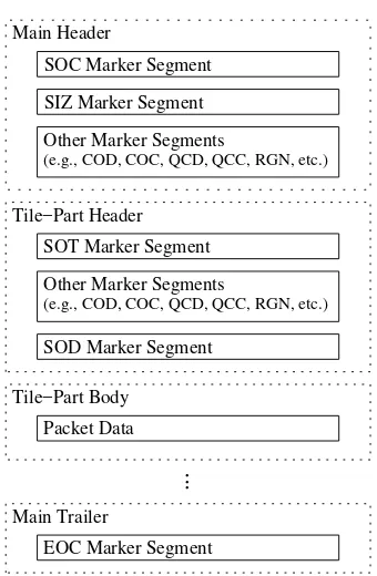
N. Code Stream
In order to specify the coded representation of an image, two different levels of syntax are employed by the codec. The lowest level syntax is associated with what is referred to as the code stream. The code stream is essentially a sequence of tagged records and their accompanying data.
Type Length (if required)
Parameters (if required)
16 bits 16 bits variable length
Fig. 13. Marker segment structure.
Main Header
Other Marker Segments Other Marker Segments
(e.g., COD, COC, QCD, QCC, RGN, etc.)
Tile−Part Header
(e.g., COD, COC, QCD, QCC, RGN, etc.)
SOC Marker Segment
SIZ Marker Segment
SOT Marker Segment
SOD Marker Segment
Tile−Part Body Packet Data
...
Main Trailer
EOC Marker Segment
Fig. 14. Code stream structure.
three fields: the type, length, and parameters fields. The type (or marker) field identifies the particular kind of marker segment. The length field specifies the number of bytes in the marker seg-ment. The parameters field provides additional information spe-cific to the marker type. Not all types of marker segments have length and parameters fields. The presence (or absence) of these fields is determined by the marker segment type. Each type of marker segment signals its own particular class of information.
A code stream is simply a sequence of marker segments and auxiliary data (i.e., packet data) organized as shown in Fig. 14. The code stream consists of a main header, followed by tile-part header and body pairs, followed by a main trailer. A list of some of the more important marker segments is given in Table II. Pa-rameters specified in marker segments in the main header serve as defaults for the entire code stream. These default settings, however, may be overridden for a particular tile by specifying new values in a marker segment in the tile’s header.
All marker segments, packet headers, and packet bodies are a multiple of 8 bits in length. As a consequence, all markers are byte-aligned, and the code stream itself is always an integral number of bytes.
O. File Format
A code stream provides only the most basic information re-quired to decode an image (i.e., sufficient information to deduce the sample values of the decoded image). While in some simple applications this information is sufficient, in other applications
LBox TBox XLBox (if required)
DBox
32 bits 32 bits 64 bits variable
Fig. 15. Box structure.
additional data is required. To display a decoded image, for ex-ample, it is often necessary to know additional characteristics of an image, such as the color space of the image data and opacity attributes. Also, in some situations, it is beneficial to know other information about an image (e.g., ownership, origin, etc.) In or-der to allow the above types of data to be specified, an additional level of syntax is employed by the codec. This level of syntax is referred to as the file format. The file format is used to convey both coded image data and auxiliary information about the im-age. Although this file format is optional, it undoubtedly will be used extensively by many applications, particularly computer-based software applications.
The basic building block of the file format is referred to as a box. As shown in Fig. 15, a box is nominally comprised of four fields: the LBox, TBox, XLBox, and DBox fields. The LBox field specifies the length of the box in bytes. The TBox field indicates the type of box (i.e., the nature of the information contained in the box). The XLBox field is an extended length indicator which provides a mechanism for specifying the length of a box whose size is too large to be encoded in the length field alone. If the LBox field is 1, then the XLBox field is present and contains the true length of the box. Otherwise, the XLBox field is not present. The DBox field contains data specific to the particular box type. Some types of boxes may contain other boxes as data. As a matter of terminology, a box that contains other boxes in its DBox field is referred to as a superbox. Several of the more important types of boxes are listed in Table III.
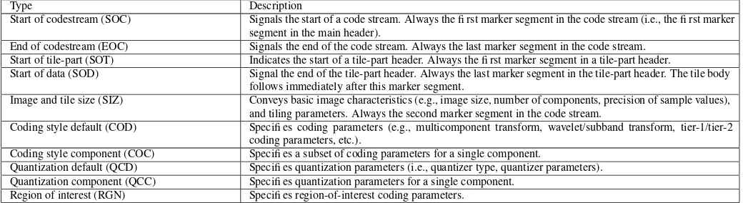
TABLE II
TYPES OF MARKER SEGMENTS
Type Description
Start of codestream (SOC) Signals the start of a code stream. Always the fi rst marker segment in the code stream (i.e., the fi rst marker segment in the main header).
End of codestream (EOC) Signals the end of the code stream. Always the last marker segment in the code stream. Start of tile-part (SOT) Indicates the start of a tile-part header. Always the fi rst marker segment in a tile-part header.
Start of data (SOD) Signal the end of the tile-part header. Always the last marker segment in the tile-part header. The tile body follows immediately after this marker segment.
Image and tile size (SIZ) Conveys basic image characteristics (e.g., image size, number of components, precision of sample values), and tiling parameters. Always the second marker segment in the code stream.
Coding style default (COD) Specifi es coding parameters (e.g., multicomponent transform, wavelet/subband transform, tier-1/tier-2 coding parameters, etc.).
Coding style component (COC) Specifi es a subset of coding parameters for a single component.
Quantization default (QCD) Specifi es quantization parameters (i.e., quantizer type, quantizer parameters). Quantization component (QCC) Specifi es quantization parameters for a single component.
Region of interest (RGN) Specifi es region-of-interest coding parameters.
File Type Box
Image Header Box
Color Specification Box JP2 Header Box
...
Contiguous Code Stream Box JPEG−2000 Signature Box
...
Fig. 16. File format structure.
and vendor/application-specific data.
Although some of the information stored at the file format level is redundant (i.e., it is also specified at the code stream level), this redundancy allows trivial manipulation of files with-out any knowledge of the code stream syntax. The file name extension “jp2” is to be used to identify files containing data in the JP2 file format. For more information on the file format, the reader is referred to [45].
P. Extensions
Although the baseline codec is quite versatile, there may be some applications that could benefit from additional fea-tures not present in the baseline system. To this end, Part 2 of the standard [15] defines numerous extensions to the base-line codec. Some of these extensions include the follow-ing: 1) additional intercomponent transforms (e.g., multidimen-sional wavelet/subband transforms); 2) additional intracompo-nent transforms (e.g., subband transforms based on arbitrary filters and decomposition trees, different filters in the horizon-tal and vertical directions); 3) overlapped wavelet transforms; 4) additional quantization methods such as trellis coded quanti-zation [46, 47]; 5) enhanced ROI support (e.g., a mechanism for explicitly signalling the shape of the ROI and an arbitrary shift value); and 6) extensions to the file format including support for additional color spaces and compound documents.
IV. CONCLUSIONS
In this paper, we commenced with a high-level introduction to the 2000 standard, and proceeded to study the JPEG-2000 codec in detail. With its excellent coding performance and many attractive features, JPEG-2000 will no doubt become a widely used standard in the years to come.
APPENDIX
I. JASPER
JasPer is a collection of software (i.e., a library and applica-tion programs) for the coding and manipulaapplica-tion of images. This software is written in the C programming language. Of particu-lar interest here, the JasPer software provides an implementation of the JPEG-2000 Part-1 codec. The JasPer software was devel-oped with the objective of providing a free JPEG-2000 codec implementation for anyone wishing to use the JPEG-2000 stan-dard. This software has also been published in the JPEG-2000 Part-5 standard, as an official reference implementation of the JPEG-2000 Part-1 codec.
The JasPer software is available for download from the JasPer Project home page (i.e., http://www.ece.uvic.ca/ ˜mdadams/jasper) and the JPEG web site (i.e.,http://www. jpeg.org/software). For more information about JasPer, the reader is referred to [8–10].
ACKNOWLEDGMENT
The author would like to thank Image Power, Inc. for their past support in the development of the JasPer software. Also, the author would like to express his gratitude to Dr. Faouzi Kossen-tini for past collaborations that led to the author’s involvement with JPEG-2000 standardization activities (hence, making a pa-per like this possible).
REFERENCES
[1] ISO/IEC 10918-1: Information technology—Digital compression and cod-ing of continuous-tone still images: Requirements and guidelines, 1994. [2] G. K. Wallace, “The JPEG still picture compression standard,”
Communi-cations of the ACM, vol. 34, no. 4, pp. 30–44, Apr. 1991.
[3] W. B. Pennebaker and J. L. Mitchell,JPEG: Still Image Data Compression Standard, Kluwer Academic, New York, NY, USA, 1992.