VARIOUS APPLICATIONS OF LINEAR ALGEBRA
H.A. Parhusip
Satya Wacana Christian University Jl. Diponegoro 55 -60 Salatiga 50711
ABSTRACT
Various applications of linear algebra are presented here. Undergraduate students in mathematics are mainly have no enough background in integrating linear algebra from different subjects and have difficulties to deal with data for applying linear algebra. On the other hand, students have learnt many properties in linear algebra but students are lacking to work with in practical sense. Therefore this paper shows some guidelines to handle this problem through some examples taken from some researchs on linear algebra by using data from surrounding.
Multivariate regression is introduced which is used to fit closing stock prices as an example. QR decomposition is recalled in order to solve a linear system with no solution in the classical linear algebra lectures.
Modelling on stevioside with a two dimensional quadratic function, logistic model of crown diameter of Kailan, discriminant analysis of foods, protein content of beans, Belousov-Zhabotinsky (BZ) reaction as a model on differential equations are some examples shown on this paper. These applications are mainly dealt with parameters determination that lead to linear system and nonlinear system. Least square and Newton method are the basic used methods in this paper which are solved by fmincon and lsqnonlin and provided by MATLAB. One needs to know a particular software language (such as MATLAB, R) to reinvent the results in this paper.
Keywords: least square, positive definite, convex-nonconvex functions,discriminant analysis, matrix covariance, eigenvalues-eigenvectors.
I. INTRODUCTION
One of big branches in mathematics is linear algebra which must be taken by each student in undergraduate mathematics. It may also be an obligation in computer science and other sciences where a numerical computation is necessary. In multivariate analysis, one will meet lots of linear algebra that we will also present in this paper.
The used data are taken from Middle Java and its surroundings such that undergaduate students may also apply to their practical problems which may be tasked by their lecturers. The other problem can also be obtained as an analysis of given models by other researchers in applied sciences.
This paper will focus on linear systems and nonlinear systems that obtained from parameters determination. Compared to some existed journals in applied of linear algebra, this paper is very narrow. There are some collections of informations (collected by Axelsson and Chen, 2011) that dealing with matrix computations and nonlinear equations require lots of numerical methods (hence many linear algebra involve). However, using data typically from Salatiga and its surroundings for implementing linear algebra is still lacking). This paper provides some examples of using linear algebra in this sense.
II. DETERMINATION OF PARAMETER ON LINEAR REGRESSION
2.1 Introduction
This part is mostly taken from (Peressini,et.all, 1988, Chapter 4). Assume we have a set of data presented on
(
t
1,
s
1),...,
(
t
n,
s
n)
and we assume that there exists a continuous function f such that s=f(t) in the form of polynomial on orderk kt x t
x x t p
In this case the independent variable is t. The variables
x
0,...,
x
k are the polynomial coefficients based on the given data. We need to findx
0,...,
x
k such that the deviation of) ( i
i p t
s as small as possible. The function must fit to all points i=1,...,n and hence the problem becomes a minimization problem in the sense of least square. This means that we have to minimize
n i k j j i j i n i i ik
s
p
t
s
x
t
x
x
x
R
1 2 0 1 2 10
,
,...,
(
)
. (2a)To proceed further, one writes the residual function (2a) in the matrix-vector notation. We may write the Eq.( 2a) using norm vector by introducing
k n n n k k t t t t t t t t t A 2 2 2 2 2 1 2 1 1 1 1 1 , n s s s b 2 1 , k x x x x 1 0 . We have
n i k j j i j i n i i ik s p t s x t
x x x R 1 2 0 1 2 1
0, ,..., ( ) = b Ax
b Ax
b Ax
2
=
b
b
2
b
A
x
A
x
A
x
=b
b
2
A
Tb
x
x
A
TA
x
.Minimizing R means that we need to solve Rwhich denotes the derivative of R with respect to each variable. Note that the unknown in this case is x0,x1,...,xk. Thus
k k
x
R
x
R
R
,...,
0=
bb2ATbxxATAx
=A
Tb
A
TA
x
2
2
. (2b)Analogously in Calculus, the minimizer of R is the value of
x
x
* whichsatisfies
0
R
. From Eq. (2b) and usingx
x
*, we get0
2
2
*
A
Tb
A
TA
x
orA
TA
x
*=A
Tb
. (2c).Thus the determination of parameter (in this case the coefficients of polynomial in Eq.
1) is deduced into a problem of solving linear system (2c). The solution
x
x
*
becomes
a minimizer if only if
A
TA
is positive definite. Additionally, the matrixA
TA
is invertible if only ifA
TA
is positive definite. Therefore we get*
x
=(
A
TA
)
1A
Tb
. (2d)2.2 Furthermore in Regression
Assume we have a dependent variable
y
=[ y1,...,yn]T and p independent variables. We put our data as a matrix random variable X with p variables X1, . . . , Xpwhere each of its coloums contains n observations.
X
X
pX
py
0 1 1 2 2...
. (1)
Each observation satisfies
i pi p i i i
i x x x x
y
0
1 1
2 1
3 1 ...
, i=1,...,n . (2) In matrix-vector notation, Eq. (2) becomes) 1 ( ) 1 ) 1 (( )) 1 ( (
1 nx p p x nx
nx Z
Consider thatZ(nx(p1)) contains 1 on the first column and the second column up to (p+1)-th column are the vector-vector X1, . . . , Xp. Regression vector
((p1)x1)
=
Tp
0 1
is obtained by employing the least square, i.e we have to minimize
21 1
0
n i
p
j
ij j
i x
y
R
. (4a)In lecture of linear algebra , we have norm notation, and hence the Eq.(4a) can be presented as
R
=
Z y Z y Z
y 2 =yy2yZ
Z
Z
. (4b) Minimizing (5b) means that we have to derive the first derivatives of (5b) with respect to each variable (in this case, the variables are
0,
1,...
p). We haveT
p R R
R
0 ,..., =
Z Z Z y y
y
2 = 2ZTy2ZTZ
0.Thus, the estimated
is obtained by solving
Z Z y
ZT T , or
Z
TZ
1Z
Ty
. (5)
Note that the invers matrix does not always exist as shown in linear algebra lecture.
Therefore we need to add the condition that
can be obtained if only if
Z
TZ
1exists which means that the minimizer R exists as long as the matrixZ
TZ
is positive definite. Additionally, theZ
TZ
is obtained from
(
R
)
R
=Z
TZ
which is the Hessian matrixof R and Z has full rank p+1n in order
Z
TZ
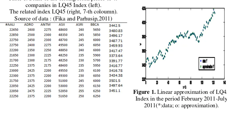
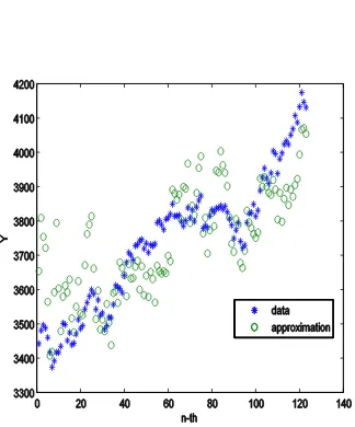
1exists (John and Wichern, 2007,page 290 for this proof).Example 1. Suppose we have the closing stock prices of 45 companies in LQ45 Index in the period of February-July 2011 (Pratama,et.all. 2011) which partly shown in Table 1. In this study, we have p= 49 variables and each variable contains n = 246 samples. Assume that LQ45 index is the respond variable Y, and we assume the LQ45 index depends linearly the closing stock prices. Thank to MATLAB that it provides us to solve Eq.(5) and hence we get the linear regression which is shown in Figure 1.
The least square approximation shows a good approximation. Which company is allowed to join LQ45 Index to the next period ?(a practical purpose). Therefore, one needs information which company contributes significantly basing on linear regression.
If the number of variables is too large, one may employ the principal component analysis to select dominant variables. This method is based on working with the largest eigenvalue of the covariance matrix and linear combination of original variables where its weights are obtained by each component of eigen vector of the largest eigenvalue. One example of using this method is stock prices analysis from 8 sectors (Parhusip, et.all. 2010).
How do we solve Eq.(5) if we do not have a positive definite matrix Z ?(In the case that we have no solution, but we have to find its approximation). One way to deal with this problem is called QR decomposition (Peressini,et.all, 1988). This method basicly decomposes Z=A = QR and denote
x
andb
Z
Ty
A
T
y
such thatAx
b
or
Z
Z
y
Z
T
T . We use Ax
b
to have a familiar notation. This method relies onRemember :
2 1
2
.x x x
x x x n
i
T
i
orthogonalization Gram-Schmidt to construct of matrix A where
A
TA
is not positive definite.Table 1. Some of the closing stock prices of 49 companies in LQ45 Index (left). The related index LQ45 (right, 7-th coloumn).
Source of data : (Fika and Parhusip,2011)
Figure 1. Linear approximation of LQ45 Index in the period February 2011-July
2011(*:data; o: approximation).
Let Q be the matrix with its column-column vectors are
) ( ) 1
( ,...,u m
u obtained by
orthogonalization Gram-Schmidt. Since Q is an orthonormal matrix m x n , hence
I
Q
Q
T
. Additionally, Q can be considered a reduced matrix A becomes Q using arelation Q=AL with L is a triangular matrix n x n. The matrix L has an invers since Q
contains independent linear coloumn-coloum vectors and denote R=
L
1 to be an upper triangular matrix n x n orR Q AT
(since QTQI
). We will use these explanations to solve
(5) , i.e
x
*= (ATA)1 ATb , with AZ , bZTy and
x
.We employ Z=QR such that we obtain
*
x
= 1)
(ZTZ ZTb=
QR QR
QR b TT 1
=
RTQTQR
RTQTb 1
= R I IQTb
1
=R QTb
1
(sinceQTQI) (6)
Note that Eq.(6) can be solved by back substitution since R is an upper triangular matrix . The last problem in the linear system is that the system contains infinitely many solutions (underdetermined system). Old fashion of linear algebra ends up to this statement. The norm minimum shows a possible solution which is considerable good enough but this topic is not shown on this paper (see Peressini, et.all, 1988, page 145-149 for detail). Note that the norm minimum relies on the invers of Gramm-matrix (
AA
T). IfA contains big numbers or rows let A have its dimension n x p, hence
A
Thas dimensionp x n. Suppose n=246 and p=2 , then the dimension of G is n x n = 246 x 246.
Example 2. Let us assume we have the closing stock prices from 2 companies given from Example 1. The dependent variable is also the LQ45 Index. Thus in this case, n = 246 with 2 independent variables. We have a linear system with Z has dimension n x (1 + 2) and the right hand side vector has dimension n x 1. We employ least square and QR
Figure 2a. The linear regression of closing stock prices from 2 companies given from Example 1 with the dependent variable is the LQ45 Index using least square.
Figure 2b. The linear regression of closing stock prices from 2 companies given from Example 1 with the dependent variable is also the LQ45 Index using QR decompotition .
III.PARAMETERS DETERMINATION ON NONLINEAR LEAST SQUARE
Modellings based on the given data mostly deal with parameters determination. Some examples are using data taken from small industries and public offices in Salatiga and its surroundings. Modelling of Total Investment and Its Efficiency in the District of Sidomukti (Parhusip, 2009a) is one example on economics. The issue of ‘sapi glonggongan’ (adding much drinking water to cows) in the year 2009 inspired us to measure an optimal weight of a cow (Parhusip and Ayunani, 2009). To achieve optimal parameters, one needs to find ‘nice’ data for optimization purposes. Hessian matrix is used to select data such that one may proceed an optimization procedure which fit to the used theories (Parhusip H. A. 2009b).
3.1 Stevioside is a promising sweetener (Parhusip and Martono, 2011)
Leaves of Stevia rebaudiana Bertoni have been extracted in Chemisty Department of Science and Mathematics Faculty, SWCU in January – March 2011 Using a quadratic function, percentage of stevioside is modelled (Parhusip and Martono, 2011) as a function of mass and time. Standard procedure of minimization problem is employed to find parameters in the objective function. We assume that the percentage of stevioside follows
2 2
) ( ) ( ) ,
(t m t m
S := S model (1)
where t and m denote time and mass respectively and the parameters
,
.
are determined due to the given data. Standard least square leads to minimize the residual function, i.e
21
mod , ,
,
,
n
i
el i data
i S
S
R =
2
1
2 2
, ( )
n
i
i i
data
i t m
S . (2)
The critical conditions require
R
0
. Solving this nonlinear system, one yields
,
,
T= (0.4201. 0.8696.- 0.0688)T. The illustration of this function is depicted on Figure 1. To get the maximum percentage stevioside from the given minimum mass will be the interest of this research. This leads to a minimax problem in optimization,i.e)
(
max
min
S
x
S x
[image:5.595.120.282.88.283.2] [image:5.595.317.492.119.264.2]As one kind of sweeteners, stevioside is promising. One good news of using stevioside is that it is not disturbing a fertility and reproduction of a user which was investigated for mice (Yodyingyuad and Bunyawong, 1991).
Figure1.
0688 . 0 ) 8696 . 0 ( ) 4201 . 0 ( ) ,
(t m t 2 m 2
S .
Since positive impact of using stevioside, study of stevioside is becoming attractive and one needs to produce stevioside into easily and savely consumed.
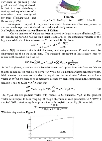
3.2 Logistic model for crown diameter of Kailan
Crown diameter of Kailan has been modeled by logistic model (Parhusip,2010). By introducing variable t as the time variable and D(t) as the dependent variable of the logistic model (which is also known as Velhust model) . We have
) 0 (
) 0 ( ,
) (
D D K A Ae K
K t
D kt
(1a)
where D(0) represents the initial diameter, and the parameters K and k must be determined based on the given data. The standard procedure of least square leads to minimize the residual function. i.e
21 data , 2
1
model , data , )
,
(
n
i
t k i
n
i
i
i K Ae i
K D
D D k
K
R . (1b)
At the first glance, it is not obvious how the system will appear from this function. Notice
that the minimization requires to solve
R
0
.This is a nonlinear homogeneous system. Matrix-vector notations will shorten the equations. Let us denote X denotes a coloum vector in
nwhere each of its components defined by each component in the summation (Eq.1b). ThusR
(
K
,
k
)
X
TX
such that
0 2
X X K R
K ; 2 0
X X k R
k . (2)
The
KX
denotes gradient vector with respect to K. Similarly,
kX
is the gradient vector with respect to k. Solving Eq.(2), we get the value of each parameter, i.e K=0.9844 and k=3.6688. Substituting these parameters in the logistic model Eq.(1), we obtain. 1.0119
9844 . 0
9844 . 0 )
( 3.6688t
e t
D
[image:6.595.108.515.125.686.2]Which is depicted on Figure 1.
Figure 1. Logistic model of Kailan’s growth with K=0.9844 dan k=3.6688 (Parhusip, 2010)
3.3 Penalty Method with a noncoercive objective function
f
(
x
)
Percentages of protein are assumed to follow a perturbed continuous function
) (x
f and its optimization follows the Lagrangian
L
(
x
,
)
forP
,i.e)
(
~
)
(
)
,
(
1x
g
x
f
x
L
m i i i
. m = the number of constraints.
Applied this construction to the studied problem, one yields
t B Y x t B Y x
L 1 2
2 ) , (
. 2 1 2 2 2 t B Y t B Y t B Y Since L(x,
)0, we obtaint
*
0
;Y
*
0
;B
*
0
.;
2* 0. SinceB
*
0
0
*
Y
, to2
B
*
1Y
*
B
* 2 = 0. One deduces2
B
*= 0 which is absolutely wrong sinceB
*
0
and
0. Thus we have shown there exists no practical true optimizer tosatisfyL(x,
)0. Therefore numerical methods in fmincon.m and fminunc.m fail. Up to now, we are dealing with optimizations that require solving of linear and nonlinear systems. There are several modern optimization algorithms avoiding these: such as anneling simulation, ant colony algorithms and genetic algorithm,particle swarm algorithm where their algorithms are inspired by nature behaviours. One may refer to (Rao.S.S.2009),(Brownlee, J. 2011)
for beginners on engineering optimization. The ant colony algorithm has been developed by some authors by renewing the steps of evaporation in this algorithm. Additionally, there exists no requirement of convexity of the objective function for using these algorithms and one should not solve of gradient function to find its optimizers. In the next section, one also requires linear algebra in statistics when we are working with data analysis.IV.LINEAR ALGEBRA ON MULTIVARIATE ANALYSIS
4.1 Discriminant Analysis (Parhusip and Natangku, 2011)
One of problems in multivariate analysis is to discriminate data into some groups. We will discuss only 2 groups. We have a set of data that contains various Indonesian foods. Protein, fat, carbohydrates , and calcium in each food have been observed. Each item of foods will be classified into 2 groups. The classification rule says that a sample
0
x is selected in a group
1 if the inequality (1) is satisfied. i.e
02 1 2 1 1 2 1 0 1 2
1
x x S x x x S x
x pooled pooled (1)
with
2
) 1 ( 1 2 1 2 2 1 1 n n S n S n Spooled
is the covariance matrix as a linear combination
between the covariance matrix from the first group denoted by
S
1and the covariancematrix from the second group denoted by
S
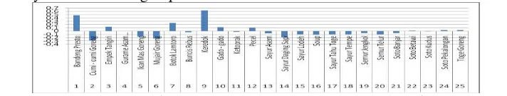
2. The formula (1) is obtained as a study of expectation cost misclassification which is omitted the discussion here for simplicity (see Johnson and Wichern, 2007 for detail).group. If the histogram too small (closes to zero) then the food can not be discriminated significantly into one of the groups.
Figure 6. Clasification of 50 foods into 2 groups (shown only the first 25th). The values on the vertical axis are the values obtained from the left hand side on Equation (1).
We expect that Figure 6 is now usable to a user. For instance, the first food (called ‘Bandeng Presto’) contains protein and fat more rather than carbohydrate and calcium.
Due to limitation of papers, other applications of linear algebra in multivariate analysis can not be shown. Joint density of multivariate variables, the maximum likelihood estimation for mean and matrix convariance, factor analysis require the invers of covariance matrix to exist. Dealing with linear combination of random multivariables require lots of knowledge in linear algebra in its general theories to a formal analysis (see John and Wichern,1997).
V. LINEAR ALGEBRA ON A SYSTEM OF DIFFERENTIAL EQUATIONS
Searching an equilibrium from a system of differential equations and eigenvalue problem lead to solve a homogeneous linear (nonlinear system). One of the studied models as a system differential equations is the Belousov-Zhabotinsky (BZ) reaction (Parhusip,2010) which its model is available in the web.
5.1 Introduction
The Belousov-Zhabotinsky (BZ) reaction is a family of oscillating chemical reactions. The non dimensional model as a system of ordinary differential equations with boundary layer, i.e
x zd dz fzx xy qy d
dy x
x xy qy d
dx
' , ;
1 ,
) 1 ( 1
. (2)
The problem (2) presents an ordinary differential equations that contains small parameters. One way is using perturbation method (Holmes,1995) which is not applied here. The way to solve this model is using Runge Kutta solver as one of standard algorithms though this algorithm may fail for a problem containing small parameters. The solutions are oscillating and periodic. These describe the nature of BZ reaction. Our interest in this research is the stability of its equilibrium point (a point that
satisfies
d
(.)
/
d
0
) .5.2 Linearization about the Equilibrium Point (Golubitsky and Dellnitz,1999)
In the linear case, an equilibrium is asymptotically stable if and only if all real eigenvalues of the matrix
A
F
'
(
X
*)
are negative. If at least one eigenvalue is real positive then the equilibrium is unstable. In the nonlinear system of differential equations, the stability is defined by the following theorem.Theorem 1. Suppose that
X
*
is an equilibrium of the system of nonlinear differential equationsX
F
X
,
. If all eigenvalues of the Jacobian matrix F'(X*)are real negative then theX
*
is an asymptotically stable. If F'(X*) has at least one real positive eigenvalue then the equilibrium is unstable.It is obvious that
T
Tz y
x*, *, * 0,0,0 is its equilibrium point. We realize that this
point has no practical meaning (since
T
T zy
x*, *, * 0,0,0 means that no used substances)
our study in this equilibrium point. Since the system is nonlinear, we need to linearize the model (3) . Using Taylor series, we expand the problem (3) near the equilibrium , the first term of right hand side is 0 by definition of equilibrium. Equation (4) becomes
d dz d dy d dx
z y x f q q
1 0
1 '
1 ' 1 0
0 1 1
. (4)
By substituting the given values of . q ,f in (4), we have a linear system and hence various values of eigenvalues. The complex eigenvalues present an existence of oscillation in the system. Therefore the study the stability near the equilibrium point will be the interest on this research. One type of stabilities is according to Lyapunov which is not shown on this paper.
VI.CONCLUSION AND REMARK
This paper has shown some examples in applications of linear algebra which particularly on linear and nonlinear regression that led to solving of linear and nonlinear systems. Some topics are discussed here : regression of stock prices-LQ45 Index as an application in economic, optimization on percentage stevioside and BZ reaction as applications in chemistry, crown diameter of Kailan as logistic model and percentage of protein in beans, foods discimination as applications in biology and food industries.
There are many more applications that one may obtain in literatures. Some topics in images proccesing and application of partial differential equations create big matrices. Working with a big matrix requires memory costly. Therefore some techniques appear in numerical methods such as factorize a full matrix into a sparse band matrix (LU decomposition, factorization QR, and Incomplete factorizations). Other possibility is by segmentation data that one can analyze separately,g.e a matrix obtained by an anisotropic images (Yunjie et.all, 2012).Thus it leads us to study of solving linear systems with big matrices and one needs knowledge on using a software to do an analysis as well as its formal theory.
REFERENCES
1. Axelsson, O. and Chen, X. 2011. Matrix computations and nonlinear equations,
Numer. Linear Algebra Appl. 2011; 18:175–176, Published online in Wiley Online Library (wileyonlinelibrary.com). DOI: 10.1002/nla.773.
2. Brownlee, J. 2011. Clever Algorithms: Nature-Inspired Programming Recipes, First Edition, Lulu Enterprises, January 2011. ISBN: 978-1-4467-8506-5.
3. Golubitsky, M and Dellnitz, M. 1999. Linear Algebra and Differential Equations Using Matlab, Brooks/Cole Pub Co.
4. Grosan,C and Abraham, A. 2008. A New Approach for Solving Nonlinear Equations Systems, IEEE Transactions on Systems, Man, and Cybernetics—part a: Systems and Humans, vol. 38, no. 3.
5. Holmes, M. H. 1995. Introduction to Perturbation Methods, Springer Verlag, New-York.
6. Johnson, R. A. and Wichern, D. 2007. Applied Multivariate Statistical Analysis, Pearson College Div.
7. Parhusip H. A. 2009a. Modelling of Total Investment and Its Efficiency in the District of Sidomukti, Proceeding of IndoMS International Conference on Mathematics and Its Applications (IICMA), ISBN:978-602-96426-0-5, 0353-0352.
Sapi, Prosiding Seminar Nasional Matematika, Vol 4, hal.AA 42-51, ISSN 1907-3909.
9. Parhusip H. A. 2009b. Data Selection with Hessian Matrix, Proceeding of IndoMS International Conference on Mathematics and Its Applications (IICMA), ISBN:978-602-96426-0-5, 0341-0352.
10. Parhusip, H. A dan Y. Martono. 2011. Kadar Steviosida Maksimum pada Waktu dan Massa yang Minimum, prosiding Sem. Nas FSM UKSW, ISSN:2087-0922, Vo.2 No.1, hal.645-650
11. Parhusip, H. A. dan Jantini Natangku. 2011. Pengelompokan Zat gisi Makanan Menggunakan Analisis Diskriminan, prosiding Sem. Nas Statistika UNDIP , ISBN 978-979-097-142-4, hal 151-161.
12. Parhusip, H.A. 2010. Stability of Beulosov-Zhabotinsky Reaction, presented
proceeding The 2nd International Conference on Chemical Science (ICCS) 2010 Universitas Gadjah Mada.
13. Parhusip, H.A. 2010. Crown Diameter of Phythoremidiation Agent by Logistic Model, proceeding on International Conference on Biotechnology and Climate Change by Logistic Model, UNS-23-24 July 2010.
14. Parhusip, H. A. Deva K. dan Bernadeta D K. 2010. Property dan Perdagangan sebagai Sektor Dominan pada Data Bursa Saham, Prosiding Seminar Nasional dan Pendidikan Sains FSM ISSN: 2087-0922, Vol.1 No.1,hal. 666-677.
15. Peressini, A.L, Sullivan, F.E., Uhl,J. 1988. The Mathematics of Nonlinear Programming, Springer Verlag, New York, Inc.
16. Pratama, F.W., Parhusip, H.A., and Sasongko, L.R. 2011. Prediksi Saham-saham Penghitung Indeks LQ45 Berdasarkan Koefisien Regresi Linear Berganda yang Signifikan dengan menggunakan Metode Stepwise Selection, Prosiding, SemNas Mat dan Pend Mt UNY, ISBN 978.979-16353-6-3, MT84-MT96.
17. Rao, S.S. 2009. Engineering Optimization, Theory and Practice, Published by John Wiley & Sons, Inc., Hoboken, New Jersey.
18. Sidi,A.1999. Linear Algebra and its Applications 298 ,99–113,
www.elsevier.com/locate/laa.
19. Yodyingyuad, V and Bunyawong, S. 1991. Effect of stevioside on growth and reproduction , Hum. Reprod. 6 : 158-165.