Are stock exchanges integrated in the world? - A critical Analysis

Munich Personal RePEc Archive

Are stock exchanges integrated in the

world? - A critical Analysis

Vijay Kumar Varadi and Nagarjuna Boppana

University of Hyderabad

May 2009

Online at

http://mpra.ub.uni-muenchen.de/15902/

UNIVERSITY OF HYDERABAD

Are stock exchanges integrated in the world?

A critical analysis

Vijay & Dr. Boppana Nagarjuna

In the recent rapid reforms made the global into a global village in nature and in terms of efficiency, transparency. The information flow in one market may affect the other markets in the world, because of its integration. In this regard, this paper explores the objective whether there is any integration of markets taken place or not. For reaching the objective, we have used rigorous time series techniques for the equal

period of data (1st January, 2001 to 30th April, 2009) of 17 stock exchanges in the world, which includes

Is Stock Exchanges are integrated in the world – Critical Analysis

V.Vijay Kumar1 and Dr. Boppana Nagarjuna2

Introduction:

Economic reforms in the process of globalization positively changes in its nature of world stock

exchanges. Many research scholars would pose a question, is stock exchanges are become integrated in

the reform period. In the recent years, the world economies are moving its own dimension, is

experiencing a new kind of financial crisis with its integrity and efficiency. Recent years are evident to

stock exchanges, stock prices are falling drastically and majority of investment in stock market and its

allied services is evaporating and no idea how it makes people miserable.

The integration of stock exchanges produces a number of significant efficiency gains, some of which are

passed on by the exchanges to their users (intermediaries, investors and issuers) in the form of lower fees,

and some of which accrue directly to users. The integration of exchanges eliminates the duplication of

costly infrastructure, thus reducing the average cost of processing a trade. The competitive constraints

imposed by other trading mechanisms and the bargaining power of users induce the integrated exchange

to pass on those cost savings to its members by reducing trading fees. Final investors can then benefit

from this reduction in the explicit costs of trading in the form of lower brokerage fees.

Many researchers are found that co-integration among national stock markets may be implied by one or

more of the following factors: less cross-country restrictions on stock investment and foreign ownership.

A question then arises here: what kind of co-integration, linear or nonlinear, are these factors supposed to

result in? So far, all of the studies on international stock market integration that adopt cointegration

1

Research Scholar, Department of Economics, University of Hyderabad. varadivk@gmail.com

2

analysis have taken the former for granted if cointegration is indeed present, while completely ignoring

the latter. Therefore, it is of importance to detect the possible existence of linear and nonlinear

cointegration among national stock markets.

However, the former studies specifies and estimates a nonlinear regression model without paying

attention to the possible non-stationarity of the regressand and the regressors that are the transformations

of the original time series. Thus the study is unable to cut loose from the problem of spurious regression

which cointegration techniques have been developed to overcome. In the latter study, the authors use the

original series and their cross-products and squares in the cointegration regression model after unit root

tests are applied to ensure that all the complex elements in the vector are integrated of the same order

(order one). Furthermore, the normality condition for employing the Johansen method is violated. Even

though the authors argue that no autocorrelation in the residuals is more important than the normality

condition, this does not mean that the latter is unimportant as finitesample critical values are computed

using normally distributed data.

In the theoretical literature, financial market integration derives from various postulates such as the law of

one price (Cournot (1927). Despite distinguishing features, these postulates share a common perspective:

if risks command the same price, then the correlation of financial asset prices and the linkage among

markets comes from the movement in the price of risks due to investors’ risk aversion. Based on these

theoretical postulates, financial integration at the empirical level is studied using several factors. Among

several others in the applied finance literature, have used the cointegration hypothesis to assess the

international integration of financial markets. Taylor and Tonks (1989) found that the cointegration

technique is useful from the perspective of the international capital asset price model. Kasa (1992)

suggested that the short-term return correlation between stock markets is not appropriate from the

The cointegration model is useful since it not only distinguishes between the nature of long-run and of

short-run linkages among financial markets, but captures the interaction between them as well. What is

striking about the empirical literature is that studies on the subject have brought to the fore various useful

perspectives relating to price equalisation, market equilibrium, market efficiency and portfolio

diversification (Chowdhry et al (2007)).

Harvey (1995) suggested that the improvement in market efficiency is consistent with increasing

integration with world markets. If markets are predictable and foreign investors are sophisticated, then

investors are likely to profit from the predictability of returns. Hassan and Naka (1996) suggest that in

cointegrated markets, price movements in one market immediately influence other markets, consistent

with efficient information sharing and free access to markets by domestic and foreign investors. Another

viewpoint is that national stock markets are different since they operate in the economic and social

environments of different countries. Accordingly, a country’s financial market is efficient when prices

reflect the fundamentals and risks of that country, rather than the fundamentals and risks of other

countries. Several studies have, however, argued that financial integration could occur due to real

economic interdependence or linkages among economic fundamentals across nations. For instance, the

profit and loss account and the balance sheet of a domestic company relying on a large volume of exports

and imports can be affected by the macroeconomic fundamentals of other countries.

Based on these considerations, the current paper attempts to detect non-linearity in the long-run

equilibrium relationship between several national stock markets. It is organized as follows.

Motivation of the study:

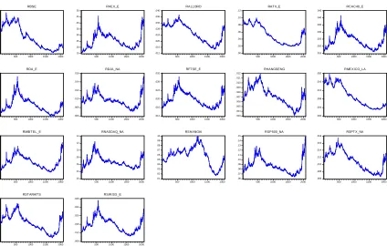
When we plot (Figure 1) the closing prices of different stock markets, we found the falling trend in all

markets at same point. It makes to go in deep, study about the reflection and affect of stock prices on

Objectives and Hypothesis:

This paper major objective is to understand the co-integration relationship between intra and inter stock

exchanges in the world and how they are integrated towards reaching the efficiency.

H0: Stock Markets are well co-integrated and leads to major fall or leads to financial crisis

H1: Otherwise

Data Sources:

World stock exchanges price series is collected and taken support from various data sources; such as

world stock exchanges, yahoo finance, BSE and its own stock exchanges for daily data of closing price

series for almost 25 major stock exchanges in the world. The data which includes ie., in Asia and Pacific

Markets we have Bombay Stock Exchange (BSE), All Ordinaries, Shangai, Hang Seng, Jakarta

Composite, KLSE, Nikkei 225, Staraits Times; in European Markets we have ATX (Vienna), CAC-40

(Paris), DAX, AEX –General (Amesterdom), MIBTEL (Milan), Swiss Market, FTSE 100; in Latin

American Markets we have MERVAL, Bovespa and IPC (Mexico) and in North American Markets

we have S&P TSX Composite, Dow Jones Index, S&P 500 index and Nasdaq-100.

Data:

The data we have considered in this paper is daily data for the period 1st January, 2001 to 30th April, 2009.

The data includes closing prices of the every stock market indices.

Methodology:

To study the above said objectives, I have followed the following methodology. First I have changed the

raw data into the return form for normalize the data. Then I have concentrated on descriptive statistics

i.e., Mean, standard deviation, minimum, maximum, skewness, kurtosis and J-B Statistic to know the

behavior of the data. After that, I just regress RBSE (return series of Bombay Stock Exchange) as a

taken place, but D-W statistics shows autocorrelation exists. I checked the correlation matrix for at what

stages all these variables correlated each other.

Although regression analysis deals with the dependence of the variable on other variables, it does not

necessarily imply causation. To find lag length of the variable, whether they have any unit root or

stationary, I have used ADF statistics with level form and ADF statistics with first difference, I found in

level form there is a unit root.

A Vector Error Correction Model:

The finding that many time series may contain a unit root has spurred the development of the theory of

non-stationary time series analysis. Engle and Granger (1987) pointed out that a linear combination of

two or more non-stationary series may be stationary. If such a stationary, linear combination exists, then

the non-stationary time series are said to be cointegrated. The stationary linear combination is called the

co-integrating equation and may be interpreted as a long-run equilibrium relationship between the

variables. Although the two series may be non stationary they may move closely together in the long run

so that the difference between them is stationary. The series RBSE and RAEX_E are said to be integrated

of the order one, denoted by I(1), if they become stationary after first difference. If there are two such

series which are I(1) integrated and their linear combination is stationary, then these two series are said to

be cointegrated. This relationship is the long run equilibrium relationship between RBSE and RAEX_E.

A principal feature of cointegrated variables is that their time paths are influenced by the extent of any

deviation from long-run equilibrium. If the system is to return to its long run equilibrium, the movement

of at least one variable must respond to the magnitude of the disequilibrium. If cointegration exists

between St and Ft, then Engle and Granger representation theorem suggests that there is a corresponding

Error Correction Model (ECM). In an ECM, the short term dynamics of the variables in the system are

The present research, seeks to determine whether there exists an equilibrium relationship between the

different indices. Engle and Granger suggest a four step procedure to determine if the two variables are

cointegrated. The first step in the analysis is to pre-test each variable to determine its order of integration,

as cointegration necessitates that the two variables be integrated of the same order. Augmented Dickey-

Fuller (ADF) test has been used to determine the order of integration. If the results in step one show that

both the series are I(1) integrated then the next step is to establish the long run equilibrium relationship in

the form

t t

t

RAEX

E

e

RBSE

=

β

₀

+

β

₁

_

+

Where RBSE is the log of Bombay stock exchange index; RAEX_E is the log of aex_E index prices at

time t and e_tis the residual term. In order to determine if the variables are cointegrated we need to

estimate the residual series from the above equation. The estimated residuals are denoted as (ê). Thus the

ê series are the estimated values of the deviations from the long run relationship. If these deviations are

found to be stationary, then the RBSE and RAEX_E series are cointegrated of the order (1,1). To test if

the estimated residual series is stationary Engle- Granger test for co-integration was performed.

The third step is to determine the ECM from the saved residuals in the previous step.

(

t t

)

RBSE t t

RBSE

e

lagged

RBSE

RAEX

E

RBSE

t

=

α

1

+

α

ˆ

1

+

∆

,

∆

_

+

ε

,,

∆

−

(

t t

)

RAEX Et

t E

RAEX

e

lagged

RBSE

RAEX

E

E

EX

_

t 1 _

ˆ

1

,

_

_ ,

A

=

α

+

α

+

∆

∆

+

ε

∆

−

In the above equations,

t

RBSE

∆

and

t E RAEX_

∆ denote, respectively, the first differences in the log of

spot and futures prices for one time period. eˆt−1is the lagged error correction term from the co-integrating

equation and

t RBSE,

ε

and

t E RAEX_ ,

The above equations describe the short-run as well as long-run dynamics of the equilibrium relationship

between spot index and futures index. They provide information about the feedback interaction between

the two variables.

In the equation

t RBSE

∆ has the interpretation that, change in

t

RBSE

is due to both, short-run effects.

From lagged futures and lagged spot variables and to the last period equilibrium error eˆt−1, which

represents adjustment to the long-run equilibrium. The coefficient attached to the error correction term

measures the single period response of changes in spot prices to departures from equilibrium. If this

coefficient is small then spot prices have little tendency to adjust to correct a disequilibrium situation.

Then most of the correction will happen in the other index prices.

The last step involves testing the adequacy of the models by performing diagnostic checks to determine

whether the residuals of the error correction equations approximate white noise. The reverse

representation of Engle and Granger’s Co-integration analysis along with the empirical findings has been

given in the appendix. A pair wise Granger Causality test was done to establish the cause and effect

relationship between the different series.

For causality, we have used Granger causality test which assumes that the information relevant to the

prediction of the respective variables. The test involves estimating the following regressions:

t j t m j j i t m i i t n i n

j t j t

i t i t

u

RBSE

E

AEX

E

AEX

u

RBSE

E

AEX

RBSE

2 1 1

1 1 1

_

_

_

+

∑

+

∑

=

∑

+

∑

+

=

− = − = = − = −

δ

λ

α

Where it is assumed that the disturbances

u

_1t and

u

_2t are uncorrelated.

Results Discussion:

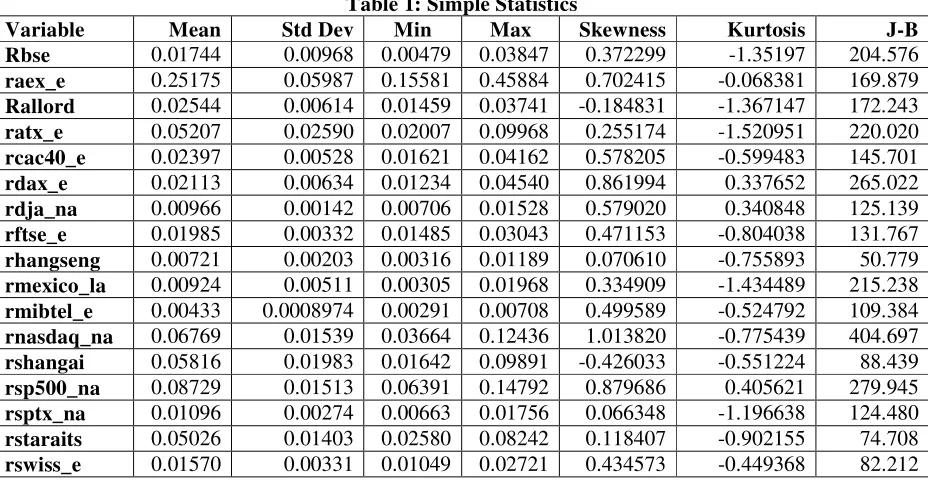
As we discussed earlier, the simple/ descriptive statistics reveals (Table 1) that all series of indices

measure of the center of the distribution of the series. Whereas, standard deviation is the measure of

degree of desperation of the data from the mean value, it indicates form the table spread exists in all

indices. Skewness is a measure of symmetry. In the given table, except rallord, rshagai (negative

skewness having left tail) all are having positive skewness, but rnasdaq_na is having positive skewness

i.e., (1.013) which indicates a long right tail exists. Kurtosis is a measure of whether the data are peaked

or flat relative to a normal distribution i.e, k=3. But in the given indices there is no such series are to be

seen. But, all the indices are negative excess kurtosis with having heavy peaked in its nature..

Table 1: Simple Statistics

Variable Mean Std Dev Min Max Skewness Kurtosis J-B

Rbse 0.01744 0.00968 0.00479 0.03847 0.372299 -1.35197 204.576

raex_e 0.25175 0.05987 0.15581 0.45884 0.702415 -0.068381 169.879

Rallord 0.02544 0.00614 0.01459 0.03741 -0.184831 -1.367147 172.243

ratx_e 0.05207 0.02590 0.02007 0.09968 0.255174 -1.520951 220.020

rcac40_e 0.02397 0.00528 0.01621 0.04162 0.578205 -0.599483 145.701

rdax_e 0.02113 0.00634 0.01234 0.04540 0.861994 0.337652 265.022

rdja_na 0.00966 0.00142 0.00706 0.01528 0.579020 0.340848 125.139

rftse_e 0.01985 0.00332 0.01485 0.03043 0.471153 -0.804038 131.767

rhangseng 0.00721 0.00203 0.00316 0.01189 0.070610 -0.755893 50.779

rmexico_la 0.00924 0.00511 0.00305 0.01968 0.334909 -1.434489 215.238

rmibtel_e 0.00433 0.0008974 0.00291 0.00708 0.499589 -0.524792 109.384

rnasdaq_na 0.06769 0.01539 0.03664 0.12436 1.013820 -0.775439 404.697

rshangai 0.05816 0.01983 0.01642 0.09891 -0.426033 -0.551224 88.439

rsp500_na 0.08729 0.01513 0.06391 0.14792 0.879686 0.405621 279.945

rsptx_na 0.01096 0.00274 0.00663 0.01756 0.066348 -1.196638 124.480

rstaraits 0.05026 0.01403 0.02580 0.08242 0.118407 -0.902155 74.708

rswiss_e 0.01570 0.00331 0.01049 0.02721 0.434573 -0.449368 82.212

The correlation matrix (table 2) reveals that, there is a positive correlation between Bombay

stock exchange index with other indices. Bombay stock index is having positive i.e., nearer to

one relationship is having allord, atx_e, sptx_na, stratits. And positive with greater than 0.5

indices are cac40_e, dax_e. dja_na, ftse_e, mibtel, nasdaq, sp500_na and swiss_e. But there is

Table 2: Cross correlations: For all Markets

RBSE RAEX_E RALLORD RATX_E RCAC40_E RDA_E RDJA_NA RFTSE_E RHANG RMEX RMIB RNASDAQ RSHANGAI RSP500_NA RSPTX_NA RSTARAITS RSWISS_E RBSE 1 0.216 0.914 0.936 0.536 0.648 0.673 0.593 0.904 0.980 0.559 0.631 0.295 0.608 0.926 0.898 0.641 RAEX_E 0.216 1 0.496 0.257 0.914 0.795 0.718 0.861 0.527 0.168 0.864 0.681 0.367 0.769 0.508 0.537 0.837 RALLORD 0.914 0.496 1 0.913 0.734 0.787 0.810 0.778 0.926 0.917 0.759 0.694 0.412 0.760 0.968 0.953 0.805 RATX_E 0.936 0.257 0.913 1 0.541 0.577 0.735 0.610 0.855 0.943 0.622 0.614 0.139 0.688 0.904 0.908 0.642 RCAC40_E 0.536 0.914 0.734 0.541 1 0.940 0.831 0.963 0.768 0.492 0.942 0.831 0.403 0.865 0.758 0.761 0.957 RDA_E 0.648 0.795 0.787 0.577 0.940 1 0.778 0.923 0.832 0.617 0.843 0.807 0.522 0.778 0.815 0.798 0.930 RDJA_NA 0.673 0.718 0.810 0.735 0.831 0.778 1 0.870 0.841 0.646 0.871 0.885 0.382 0.980 0.827 0.889 0.872 RFTSE_E 0.593 0.861 0.778 0.610 0.963 0.923 0.870 1 0.808 0.554 0.928 0.858 0.379 0.901 0.801 0.815 0.970 RHANG 0.904 0.527 0.926 0.855 0.768 0.832 0.841 0.808 1 0.864 0.774 0.807 0.485 0.797 0.946 0.952 0.827 RMEX 0.980 0.168 0.917 0.943 0.492 0.617 0.646 0.554 0.864 1 0.513 0.567 0.295 0.569 0.911 0.881 0.605 RMIB 0.559 0.864 0.759 0.622 0.942 0.843 0.871 0.928 0.774 0.513 1 0.802 0.318 0.902 0.779 0.799 0.928 RNASDAQ 0.631 0.681 0.694 0.614 0.831 0.807 0.885 0.858 0.807 0.567 0.802 1 0.342 0.915 0.760 0.784 0.829 RSHANGAI 0.295 0.367 0.412 0.139 0.403 0.522 0.382 0.379 0.485 0.295 0.318 0.342 1 0.286 0.410 0.374 0.382 RSP500_NA 0.608 0.769 0.760 0.688 0.865 0.778 0.980 0.901 0.797 0.569 0.902 0.915 0.286 1 0.788 0.844 0.887 RSPTX_NA 0.926 0.508 0.968 0.904 0.758 0.815 0.827 0.801 0.946 0.911 0.779 0.760 0.410 0.788 1 0.962 0.828 RSTARAITS 0.898 0.537 0.953 0.908 0.761 0.798 0.889 0.815 0.952 0.881 0.799 0.784 0.374 0.844 0.962 1 0.838 RSWISS_E 0.641 0.837 0.805 0.642 0.957 0.930 0.872 0.970 0.827 0.605 0.928 0.829 0.382 0.887 0.828 0.838 1

Table 3: Regression results

Dependent Variable: RBSE Method: Least Squares Sample: 1 2061

Included observations: 2061

Variable Coefficient Std. Error t-Statistic Prob.

C -0.001877 0.000511 -3.676565 0.0002

RAEX_E -0.009936 0.002503 -3.969651 0.0001

RALLORD 0.182827 0.027857 6.562946 0.0000

RATX_E -0.004735 0.007179 -0.659570 0.5096

RCAC40_E 0.083059 0.041364 2.007985 0.0448

RDA_E -0.143537 0.023610 -6.079523 0.0000

RDJA_NA 0.668038 0.187994 3.553507 0.0004

RFTSE_E -0.554943 0.044480 -12.47632 0.0000

RHANGSENG 1.773305 0.060411 29.35384 0.0000

RMEXICO_LA 0.770191 0.051565 14.93622 0.0000

RMIBTEL_E -0.398041 0.135576 -2.935923 0.0034

RNASDAQ_NA 0.132507 0.007591 17.45558 0.0000

RSHANGAI -0.052620 0.002936 -17.92480 0.0000

RSP500_NA -0.235353 0.022091 -10.65362 0.0000

RSPTX_NA 0.911251 0.058433 15.59482 0.0000

RSTARAITS 0.045955 0.011213 4.098336 0.0000

RSWISS_E 0.456324 0.043808 10.41651 0.0000

Adjusted R-squared 0.986067 S.D. dependent var 0.009678

S.E. of regression 0.001142 Akaike info criterion -10.70320

Sum squared resid 0.002667 Schwarz criterion -10.65676

Log likelihood 11046.65 F-statistic 9113.088

Durbin-Watson stat 0.166991 Prob(F-statistic) 0.000000

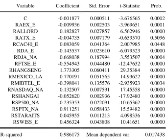
The regression results (table 3) reveal that, majority of the variables are significant at 1% level, even

though there is high t-statistic evidence this and also r-square, adjusted r-square is also evidence the same

picture about the results. But when we look at the D-W stat with 0.166991 indicates, the regression is

having a spurious regression i.e., having high t-values, high r-square and adjusted r-square and F-statistic .

It indicates that there is a non-stationary occurs among the series. However, that the long-term

information contained in levels time series will be lost after the differencing. To avoid loss of long-term

information, the majority of economists insisted on working with levels instead of differences.

Table 4: Augmented Dickey Fuller Test Statistic

Variable In level form

(with intercept and trend) ADF Statistic

First Difference (With intercept) ADF Statistic

Rbse -1.9567 -32.65831

raex_e -1.009637 -23.00168

rallord 0.101336 -47.44972

ratx_e 0.286237 -42.83707

rcac40_e -0.954035 -22.27270

rdax_e -2.136046 -47.39743

rdja_na -0.615159 -26.25541

rftse_e -1.125754 -21.69613

rhangseng -2.434619 -46.78170

rmexico_la -1.378196 -40.86398

rmibtel_e -0.544494 -15.95365

rnasdaq_na -2.360269 -35.94068

rshangai -1.462871 -45.11517

rsp500_na -0.459460 -26.70852

rsptx_na -0.673454 -48.53236

rstaraits -1.067458 -44.83061

rswiss_e -0.574758 -21.71180

Critical values in level form -3.9625 at 1%, -3.4119 at 5%, and -3.1279 at 10%

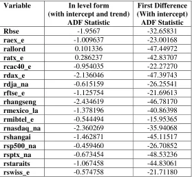
An augmented Dickey Fuller (ADF) test with 4 lags of the dependent variable in a regression equation on

the return data series with a intercept and trend, results indicate that the test statistic less than the crucial

values in the level form at least at 10% level. But, if I repeat the same process in the first difference with

intercept not with trend, all series are exceeds the test statistic critical values. So the null hypothesis of a

unit root in the all the series cannot be rejected. The test statistic is more negative than the critical value

and hence the null hypothesis of a unit root in the returns is convincingly rejected. Since the dependent

variable in this regression is non-stationary, it is not appropriate to examine the coefficient standard errors

or their ratios. Unit roots can be obtained by estimating the shift dates running a properly augmented

Dickey–Fuller (ADF) regression (Table 4); the critical values depend on the shift dates and the power of

the tests declines as the maximum number of allowed shifts (which is assumed to be known) increases.

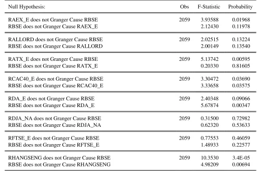
Table 5: Pair-wise Granger Causality Tests

Null Hypothesis: Obs F-Statistic Probability

RAEX_E does not Granger Cause RBSE 2059 3.93588 0.01968

RBSE does not Granger Cause RAEX_E 2.12430 0.11978

RALLORD does not Granger Cause RBSE 2059 2.02515 0.13224

RBSE does not Granger Cause RALLORD 2.00149 0.13540

RATX_E does not Granger Cause RBSE 2059 5.13742 0.00595

RBSE does not Granger Cause RATX_E 0.20330 0.81605

RCAC40_E does not Granger Cause RBSE 2059 3.30472 0.03690

RBSE does not Granger Cause RCAC40_E 3.33658 0.03575

RDA_E does not Granger Cause RBSE 2059 2.40348 0.09066

RBSE does not Granger Cause RDA_E 5.67874 0.00347

RDJA_NA does not Granger Cause RBSE 2059 0.31500 0.72982

RBSE does not Granger Cause RDJA_NA 0.62320 0.53633

RFTSE_E does not Granger Cause RBSE 2059 0.77553 0.46059

RBSE does not Granger Cause RFTSE_E 1.48933 0.22577

RHANGSENG does not Granger Cause RBSE 2059 10.3530 3.4E-05

RMEXICO_LA does not Granger Cause RBSE 2059 11.6726 9.1E-06

RBSE does not Granger Cause RMEXICO_LA 9.18103 0.00011

RMIBTEL_E does not Granger Cause RBSE 2059 2.13096 0.11899

RBSE does not Granger Cause RMIBTEL_E 3.49238 0.03061

RNASDAQ_NA does not Granger Cause RBSE 2059 1.88499 0.15209

RBSE does not Granger Cause RNASDAQ_NA 2.24799 0.10587

RSHANGAI does not Granger Cause RBSE 2059 2.07382 0.12597

RBSE does not Granger Cause RSHANGAI 2.68248 0.06863

RSP500_NA does not Granger Cause RBSE 2059 0.46386 0.62892

RBSE does not Granger Cause RSP500_NA 0.10915 0.89661

RSPTX_NA does not Granger Cause RBSE 2059 1.77191 0.17027

RBSE does not Granger Cause RSPTX_NA 9.27591 9.8E-05

RSTARAITS does not Granger Cause RBSE 2059 0.49231 0.61129

RBSE does not Granger Cause RSTARAITS 8.81523 0.00015

RSWISS_E does not Granger Cause RBSE 2059 1.34510 0.26074

RBSE does not Granger Cause RSWISS_E 1.75901 0.17247

Causality between any pair of variables there is a possibility of unidirectional causality or

bidirectional causality or none. The primary-condition for applying Granger Causality test is to

ascertain the stationarity of the variables in the pair. The second requirement for the Granger

Causality test is to find out the appropriate lag length for each pair of variables.

For this purpose, we used the vector auto regression (VAR) lag order selection. Finally, the result

of Granger causality test is reported in table 5. There is a unidirectional causal influence between

Indian stock indices and AEX, ATX_E, Hangseng, Mexico_LA, Mibtel, Shangai, Staraits. There

is no causal relationship between Indian stock indices and Allord, DJA_NA, FTSE_E,

SP500_NA. But there is bi-directional causal relationship between CAC40_E, DAX_E,

NASDAQ_NA, SPTX_NA and SWISS_E. The present study found that direction of causality is

Co-integration test results:

The valuable contribution of the concepts of unit root, co-integration, etc., is to force us to find

out if the regression residuals are stationary. In the language of co-integration theory, a

regression known as co-integration regression and the parameter is known as the co-integrating

parameter. As the unit root tests try to examine the presence of stochastic trend of time series, co

integration tests search for the presence of a common stochastic trend among the variables from

the unit root test results, the required condition for co integration test that given series are not I

(O) is satisfied. At levels all the variables are non-stationary, where as first differenced

stationary. Majority of the cases, if two variables that are I(1) are linearly combined, then the

combination will also be I(1). In general, if variables with difference orders of integration are

combined, the combination will have an order of integration equal to the largest.

A set of variables is defined as co-integrated if a linear combination of them is stationary. Many

time series are non-stationary but ‘move together’ over time – that is, there exist some influences

on the series, which imply that the series are bound by some relationship in the long run. A

co-integration relationship may also be seen as a long-term or equilibrium phenomenon, since it is

possible that co-integrating variables may deviate from their relationship in the short run, but

their association would return in the long run (Chris Brooks, 1995).

To analyze long run relationship between Indian stock Market and other stock markets, Johansen

co-integration model has adopted. For testing co-integration, there are two test statistics to use.

First, trace statistics and other is Maximum Eigen value statistics. The results are shown in table

5. An empirical result of trace statistic indicates that the rejection of null hypothesis at 0.05

long relationship with other markets. Trace test also indicates that four co-integration equations

at 1% level and one co-integration equation at 5 % level of significance, tells about long run

equilibrium between Bombay stock exchange and other markets.

Table 6: Multivariate co-integration Unrestricted Rank Test (Trace)

Hypothesized Trace 0.05

No. of CE(s) Eigenvalue Statistic Critical Value Prob.**

None 0.113150 1371.519 NA NA

At most 1 0.104365 1124.635 NA NA

At most 2 0.083718 898.0177 NA NA

At most 3 0.067779 718.2603 NA NA

At most 4 0.053064 573.9602 NA NA

At most 5 * 0.046007 461.8589 334.9837 0.0000

At most 6 * 0.041605 365.0233 285.1425 0.0000

At most 7 * 0.030684 277.6538 239.2354 0.0003

At most 8 * 0.026532 213.5790 197.3709 0.0060

At most 9 0.019171 158.2935 159.5297 0.0583

At most 10 0.017531 118.4960 125.6154 0.1251

At most 11 0.013125 82.13194 95.75366 0.2969

At most 12 0.012402 54.96791 69.81889 0.4204

At most 13 0.006529 29.30985 47.85613 0.7534

At most 14 0.004036 15.84192 29.79707 0.7234

At most 15 0.003645 7.526611 15.49471 0.5173

At most 16 9.04E-06 0.018596 3.841466 0.8914

**MacKinnon-Haug-Michelis (1999) p-values

Similarly, the empirical results of Maximum Eigen value are shown in the table 6. The empirical

result indicates that the rejection of null hypothesis at 0.05 critical value i.e. no-co integration

vector. It also tells that Bombay stock exchange have long run equilibrium with other markets.

Maximum Eigen value indicates that two co-integration equations at 1% and one co-integration

Table 7: Multivariate Unrestricted Cointegration Rank Test (Maximum Eigenvalue)

Hypothesized Max-Eigen 0.05

No. of CE(s) Eigenvalue Statistic Critical Value Prob.**

None 0.113150 246.8843 NA NA

At most 1 0.104365 226.6174 NA NA

At most 2 0.083718 179.7574 NA NA

At most 3 0.067779 144.3001 NA NA

At most 4 0.053064 112.1012 NA NA

At most 5 * 0.046007 96.83559 76.57843 0.0003

At most 6 * 0.041605 87.36951 70.53513 0.0007

At most 7 0.030684 64.07480 64.50472 0.0549

At most 8 0.026532 55.28551 58.43354 0.0991

At most 9 0.019171 39.79754 52.36261 0.5079

At most 10 0.017531 36.36404 46.23142 0.3765

At most 11 0.013125 27.16403 40.07757 0.6214

At most 12 0.012402 25.65806 33.87687 0.3420

At most 13 0.006529 13.46793 27.58434 0.8575

At most 14 0.004036 8.315304 21.13162 0.8834

At most 15 0.003645 7.508015 14.26460 0.4309

At most 16 9.04E-06 0.018596 3.841466 0.8914

Empirical analysis Error Correction Mechanism:

From the above analysis, it has explained that, Indian capital market has long run relationship

with other developing markets. But that does not mean they have short run equilibrium. There

may exists short run dynamics among capital markets. For taking care of short run equilibrium

Error Correction Mechanism (ECM) has been adopted. ECM empirical results have shown in the

table (6). Indian capital market and Australian capital market has taken into consideration.

Empirical result shows that coefficient of difference closing price ATX-100 is non-zero that

means difference closing price Sensex is out of equilibrium. Since co-efficient of lagged residual

is negative, the term θ_{ut-1is negative. Therefore, the dependent variable X is also negative to}

falling in the next period to correct the equilibrium error. Empirical result also finds that Indian

capital market adjusts to change in Australian capital market have a positive impact on short-run

changes. Similarly, in case of UK, Japan and France, short run changes in the capital market has

positive impact on short-run changes in Indian capital market except USA capital market which

has shown negative impact on short run changes in Indian capital market.

Vector Error Correction estimates

Cointegrating Eq: CointEq1

RBSE(-1) 1.000000

RAEX_E(-1) 0.055373

(0.02067)

[ 2.67931]

RALLORD(-1) -1.091942

(0.21132)

[-5.16732]

RATX_E(-1) -0.035879

(0.05483)

[-0.65437]

RCAC40_E(-1) 1.890385

(0.38265)

[ 4.94027]

RDA_E(-1) 0.121756

(0.19005)

[ 0.64063]

RDJA_NA(-1) 1.606171

(1.40853)

[ 1.14032]

RFTSE_E(-1) 0.842189

(0.35916)

[ 2.34490]

RHANGSENG(-1) -2.511124

(0.46817)

[-5.36375]

RMEXICO_LA(-1) 0.008306

(0.40725)

[ 0.02039]

RMIBTEL_E(-1) 2.219601

(1.07268)

[ 2.06921]

RNASDAQ_NA(-1) -0.297622

[-5.12900]

RSHANGAI(-1) 0.044028

(0.02170)

[ 2.02881]

RSP500_NA(-1) -0.192976

(0.16733)

[-1.15324]

RSPTX_NA(-1) 1.558806

(0.45090)

[ 3.45713]

RSTARAITS(-1) -0.010596

(0.08544)

[-0.12402]

RSWISS_E(-1) -4.050963

(0.35075)

[-11.5495]

C 0.008051

Figure 1: Return values of different stock indices

.004 .008 .012 .016 .020 .024 .028 .032 .036 .040

500 1000 1500 2000

RBSE .15 .20 .25 .30 .35 .40 .45 .50

500 1000 1500 2000

RAEX_E .012 .016 .020 .024 .028 .032 .036 .040

500 1000 1500 2000

RALLORD .00 .02 .04 .06 .08 .10 .12

500 1000 1500 2000

RATX_E .015 .020 .025 .030 .035 .040 .045

500 1000 1500 2000

RCAC40_E .012 .016 .020 .024 .028 .032 .036 .040 .044 .048

500 1000 1500 2000

RDA_E .006 .008 .010 .012 .014 .016

500 1000 1500 2000

RDJA_NA .012 .016 .020 .024 .028 .032

500 1000 1500 2000

RFTSE_E .003 .004 .005 .006 .007 .008 .009 .010 .011 .012

500 1000 1500 2000

RHANGSENG .000 .004 .008 .012 .016 .020

500 1000 1500 2000

RME XICO_LA .002 .003 .004 .005 .006 .007 .008

500 1000 1500 2000

RMIBT EL_E .02 .04 .06 .08 .10 .12 .14

500 1000 1500 2000

RNASDAQ_NA .01 .02 .03 .04 .05 .06 .07 .08 .09 .10

500 1000 1500 2000

RSHANGAI .06 .07 .08 .09 .10 .11 .12 .13 .14 .15

500 1000 1500 2000

RSP500_NA .006 .008 .010 .012 .014 .016 .018

500 1000 1500 2000

RSPTX_NA .02 .03 .04 .05 .06 .07 .08 .09

500 1000 1500 2000

RSTARAITS .008 .012 .016 .020 .024 .028

500 1000 1500 2000

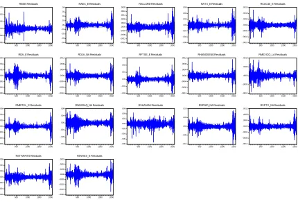
Figure 2: Residual series of stock indices -.002 -.001 .000 .001 .002 .003

500 1000 1500 2000

RBSE Residuals -.04 -.03 -.02 -.01 .00 .01 .02 .03 .04

500 1000 1500 2000

RAEX_E Residuals -.0016 -.0012 -.0008 -.0004 .0000 .0004 .0008 .0012 .0016 .0020

500 1000 1500 2000

RALLORD Residuals -.006 -.004 -.002 .000 .002 .004 .006

500 1000 1500 2000

RATX_E Residuals -.0015 -.0010 -.0005 .0000 .0005 .0010 .0015

500 1000 1500 2000

RCAC40_E Residuals -.003 -.002 -.001 .000 .001 .002 .003

500 1000 1500 2000

RDA_E Residuals -.0012 -.0008 -.0004 .0000 .0004 .0008 .0012

500 1000 1500 2000

RDJA_NA Residuals -.002 -.001 .000 .001 .002 .003

500 1000 1500 2000

RFTSE_E Residuals -.0012 -.0008 -.0004 .0000 .0004 .0008 .0012

500 1000 1500 2000

RHANGSENG Residuals -.0010 -.0005 .0000 .0005 .0010

500 1000 1500 2000

RMEXICO_LA Residuals -.0006 -.0004 -.0002 .0000 .0002 .0004 .0006

500 1000 1500 2000

RMIBTEL_E Residuals -.012 -.008 -.004 .000 .004 .008

500 1000 1500 2000

RNASDAQ_NA Residuals -.008 -.006 -.004 -.002 .000 .002 .004 .006

500 1000 1500 2000

RSHANGAI Residuals -.010 -.005 .000 .005 .010

500 1000 1500 2000

RSP500_NA Residuals -.0012 -.0008 -.0004 .0000 .0004 .0008 .0012

500 1000 1500 2000

RSPTX_NA Residuals -.006 -.004 -.002 .000 .002 .004 .006

500 1000 1500 2000

RSTARAITS Residuals -.0020 -.0015 -.0010 -.0005 .0000 .0005 .0010 .0015

500 1000 1500 2000

RSWISS_E Residuals

Figure 3: Co-integration analysis for the above said equation

-.03 -.02 -.01 .00 .01 .02

250 500 750 1000 1250 1500 1750 2000

Concluding Remarks:

This paper empirically investigates the long run equilibrium relationship between the Indian

stock market and the stock market indices of five developed countries as a using the multivariate

co integration. The multivariate co integration technique is used to investigate the long run

relationship. To assess the short run influence of one market on the other and to assess how many

days each market takes to factor out the influence Indian market, we have used the granger

causality test with two days.

The study concludes, that India and other countries markets highly co integrating during the

period of the study. Financial integration is key to delivering competitiveness, efficiency and

growth. But Is integration brings financial stability? Not necessarily. As it indicates that, the

integration of markets may also have positive impact of financial crisis which happened all over

References:

Bekaert G. and Harvey C.R. (1995): Time Varying World Market Integration: Journal of Finance. 50. pp 403-414.

Chowdhry, T, Lin Lu and Ke Peng (2007): “Common stochastic trends among Far astern stock prices: effects of Asian financial crisis”, International Review of Financial Analysis, vol 16.

Cournot, Augustin (1927): Researches into the Mathematical Principles of the Theory of Wealth, Nathaniel T Bacon (trans), Macmillan.

Hassan, M K and A Naka (1996): “Short-run and long-run dynamic linkages among international stock markets”, International Review of Economics and Finance, vol 5, no 1.

Kasa, K (1992): “Common stochastic trends in international stock markets”, Journal of Monetary Economics, vol 29, pp 95–124.

Kim, E Han and V Singhal (2000): “Stock market opening: experience of emerging economies”, Journal of Business, vol 73, pp 25–66.