Physics Page 213 THE MEASURENMENT OF ELECTRICITY AND DIELECTRIC
CHARACTERISTIC OF ONION (Allium cepa)
Abd. Wahidin Nuayi1*, Farly Reynol Tumimomor2
1Departement of Physics, Faculty of Mathematics and Natural Sciences, State University of Gorontalo,
Gorontalo, Indonesia
2Departement of Physics, Faculty of Mathematics and Natural Sciences, State University of Manado,
Minahasa, Indonesia
Abstract
This experiment aimed to measurenment of the electricity and dielectric characteristic of onion (Allium cepa). In this study, the onion have been done through the variation of frequency and temperature. The frequency was setup in 30 different values from 100 Hz -1 MHz with the temperature are from 26 0 C up to 40 0C with each increase of 2 0C. The measurement was performed
on AC current in 1 kHz and input voltage is one volt. The ions through to the membrane was measured as a conductance value by using LCRmeter that connected with two pieces of AgCl electrodes on both side of the membrane. Beside that, the conductance (G) was measured by the variation temperature of the solution. The results based on the electric characteristics variation of the frequency shows that the electricity of the onion membrane from the conductance itself is tend to increase and the capacitance is decrease due to increasing of the frequency. However, the conductance nad the capacitance of the soaked onion membrane is increase doe to increase of the temperature than the original onion membrane. In adddition, the increasing of conductance to temperature was plotted on ln G to 1/T curve. The slope or gradient of the curve is used to determine the chnage of the self-energy of the membrane and its pore radius. Self-energy of ion which obtained from non-washed and washed and soaked (with distilled water) membrane is respectively 7,66967 x 10⁻²¹ J or 0,04787 eV dan 1,2156 x
10-19 J or 0,7869 eV ( 1 joule = 6,2415 x 10¹⁸ eV) and the average of pore membrane radius is 2,00 x
10-9 meter (2,00 nm) and 1,26 10-10 meter (0,126 nm). Based on the results the onion membrane could
be a good membrane for established the electrisity anf the dielectricity.
Keyword : Electrical conductivity, Dielectric constant, Onions
1. Introduction
Membrane is a thin skin or a thin sheet of material that serves to separate the material based on the size and shape of the molecule. The membrane also hold the components of the material that has a larger size than the pores of the membrane and skip the parts on its smaller
size. The membrane has a thickness is abou 100μm to several millimeters (Pabby et al., 2009).
The membrane is also can be a separator that separates the two phases as a transport restraint the selectivity of various chemical compounds. The mixture might be homogeneous or heterogeneous, symmetric or asymmetric structure, solid or liquid, have a positive or negative charge, and also polar or neutral.
Physics Page 214
impact of the electric field pulse on the membrane tissue onions can caused by an increased of ion and its may affect to the changes of membrane permeability (Ersus et al.,2010).
The performance of a membrane is determined by the surface structure of the membrane sublayer. The electrical properties of the membrane can be seen by measuring the inductance, capacitance, impedance and the coefficient loss (Nuwaiir et al., 200). The Membrane characteristics is determined the effectiveness of the membrane in a process of separation and purification. It is very important to improve the efficiency of a system that uses membrane as one of its components. Therefore, we need an adequate membrane characterization methods (Mamat et al.,2000).
In this study aims to determine the characterization of the onion membrane that will be done by testing on electrical and dielectric properties such as conductance, capacitance, and the membrane porosity of onions.
2. Materials and Methods
2.1. Membrane Preparations
The onion membrane is the inner and outer fleshyscaleleaf layer (layer that separates between midrib / leaf meat with midrib others). The membrane were taken carefully to prevent the leakage and the damaged. The size of the membrane is taken approximately 2.5 cm x 2.5 cm. After that the membranes soaked in a solution of distilled water for 12 hours, and the other membran was not soaked as an initial.
2.2. Measurements of Conductance, Capacitance and Porosity
Pieces of parallel plate was made of pcb board with a size of 2.5 cm x 2.2 cm. The test chamber with a hole area is about 0.9 cm2. The chamber type was used a horizontal type. The conductance and capacitance was measured using LCRmeter Hioki300 models with a range of 5 MHz. The conductance was measured on a medium chamber, with KCl electrolyte solution flowing across the membrane. Part of the active layer membrane exposed to the KCl solution with a molarity higher at 1 mM and the other side with a solution of 0.1 mM KCl, where the flow of ions to flow from high to low molarity.
The amount of the ions flow through the membrane was measured as its conductance by using LCRmeter connected with 2 pieces AgCl electrodes on both sides of the membrane. The measurements were taken at a frequency of 1 kHz AC with an input voltage is about 1V. The conductance (G) was measured by the variations of temperature in a solution (T) 26-40 0C. To heat the KCl solution, the chamber was placed on a waterbath glass filled a pure water, which is heated using electric heaters. The measurement processes of the conductance has shown in Figure 4. The increasing of the conductance against the temperature was plotted in the ln G curve against 1 / T. However, the slope or the gradient of the curve is used to determine the changes of energy self-membranes and the radius of the membrane pore.
Changes of energy-self (ΔU) membrane is determined by the following equation:
ΔU = B k 1
Physics Page 215
� = � � �
� �0��∆� 2
With:
B = Radius of the membrane pores (m)
z = Ion valency (untuk KCl = 1)
q = Ion charge (1.6 x 10⁻¹⁹ C)
α = Geometric and dielectic constant (approach 0.2)
εo = Vacuum permittivity / diffusion constant (8.85 x 10⁻¹² F/m) εm = Dielectric constant of the membrane (Cahyani et al., 2012)
Figure 1 Measurement of membrane conductance
3. Result and Discussion
3.1. Effect of Frequency on the Conductance and Capacitance
Membrane conductance values of onions which were unsoaked and soaked in distilled water for 12 hours will increase as the frequency increases, as shown in Figure 2 and Figure 3. The increases of the frequency make the movement of cargo and ions in the membrane will increase, this process will boost the mobility of the membrane so that conductivity will increase.
Figure 2. The relationship between the frequency and the conductance of the original
onion
Figure 3. The relationship between the frequency and the conductance of the soaked
onions
Figure 4 shows that the conductance of the washed and soaked membrane for 12 hours in a solution of distilled water is higher than the original membrane. It is assume that when the onion membranes are washed and soaked with a solution of distilled water, the epidermis which has a supple and pliant nature experience a reduction in flexural properties and clayed.
The membrane cell can be modeled with an electric circuit consisting of a combination of capacitors and resistors (Young et al., 2003).
Physics Page 216
Figure 4. The conductance of the soaked and the original onion
Figure 5. The relationship between the frequency and the capacitance of the soaked
and the original onion.
Figure 6. The relationship between the frequency and the capacitance of soaked onion
Figure 7. The capacitance of the soaked onion and the original one
The series combined between Z1 and Z2 and the Zm formulation, it will produce the membrane capacitance.
3
where the ω = 2πf is the angular of the frequency so that the capacitance depends on the frequency.
Frequency have affected on the material itself (in this case is the membrane onion), i.e There are more waves are transmitted each second by the increasing of the frequency. The mechanisms in parallel has been occured when the direction of the electic current has been turned around before the capacitor is fully charged. So it was rapidly discharging cargo of the capacitor electrode plate.
Physics Page 217
material is inversely proportional to the dielectric constant, thereby the onions impaired dielectric constant than the density of free charge in the chip of the electrode.
3.2 Effect of Temperature on Conductance Value
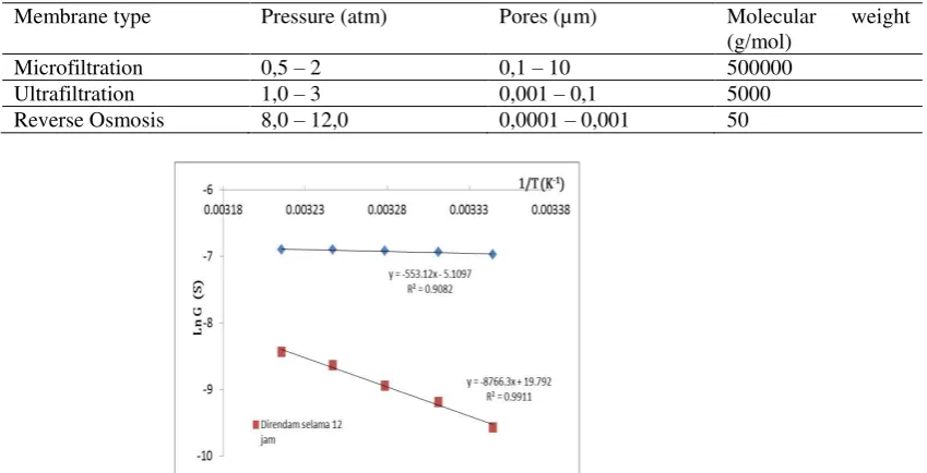
Figure 8 shows that the data generated plot tend to be in a straight line with a negative slope for the original membrane and membrane which is soaked in a solution of distilled water for 12 hours in a row at -553.12 and -8766.3 respectively. The slope values proportional to the value of the energy barrier. This indicates that the value of the conductance has dependence
on temperature with energy change ΔU themselves to the membrane without soaked and
washed and soaked in a solution of distilled water in a row of 553.12 J / K and 8766.3 J / K.
The rise of the temperature increase the kinetic energy, which can be concluded that the faster movement of ions will increase the membrane conductance values and it is ultimately will affect the characteristics of the membrane itself. By using equation (1), a slope of the curve is used to determine the energy self-ion obtained for unsoaked and unwashed membranes and soaked membranes in a solution of distilled water in a row of 7.66967 x 10⁻²¹ J or 0.04787 eV and 1.2156 x 10⁻¹⁹ J or 0.7869 eV (1 joule = 6.2415 x 10¹⁸ eV) respectively.
Table 2 The range of the pressures, pore, and the molecular weight of the various types of membranes . [Mulder (1996), Porter (1990) ]
Membrane type Pressure (atm) Pores (µm) Molecular weight
(g/mol)
Microfiltration 0,5 – 2 0,1 – 10 500000
Ultrafiltration 1,0 – 3 0,001 – 0,1 5000
Reverse Osmosis 8,0 – 12,0 0,0001 – 0,001 50
Figure 8. The relationship between temperature and the conductance of the soaked and original onion
4. Conclusion
Physics Page 218 References
Chahyani, R. . 2012. Sintesis dan Karakterisasi Membran Polisulfon Didadah Karbon Aktif untuk Filtrasi Air [Synthesis and Caracterisation of Polysulfone Membrane Didadah Activated Carbon on Water Filtration]. Sekolah Pascasarjana Institut Pertanian Bogor. [Bahasa Indonesia] [Thesis]
Ersus, B. 2010. Determination of Membrane Integrity in Onion Tissues treated by Pulsed Electric Field:Innovative Food Science & Emerging Technologies, Pages 598–603. Access on 17 April 2014 http://www.mendeley.com/research/determination-membrane-integrity-onion-tissues-treated-pulsed-electric-fields-microscopic-images ion-leakage-measurements (Online Article)
Giancoli, Douglas. 2001. Fisika Jilid 2 Edisi Kelima [Physiscs Fifth Edition] Yulhilza Hanum, Irwan Arifin, Translator Jakarta: Erlangga. [Bahasa Indonesia, Translate from Physiscs Fifth Edition.] ISBN 979-688-133-0
Mamat, Rahmat. 2000. Penentuan Impedansi Membran Pada Berbagai Konsentrasi Larutan
Eksternal Dengan Metode Spektroskopi Impedansi.[Impedance Determination Membrane Solutions at Various Concentrations External Impedance Spectroscopy Method]. Physics Departement Faculty of Mathematics and Natural Science Bogor:Institute of Agriculture Bogor. [Bahasa Indonesia] [Thesis]
Mulder, Marcel.1996. Basic Principles of Membrane Technology, Kluwer Academic Publishers, London, pp. 51 – 59, pp. 307 – 319, pp. 465 – 479.
Pabby, Anil K, S. S. H. Rizvi and A. M. Sastre. 2009.Handbook of Membrane Separations Chemical, Pharmaceutical, Food, and Biotechnological Applications, CRC Press Taylor & Francis Group, New York, pp. 66 – 100.
Porter, M.C. 1990. Handbook of Industrial Membrane Technology. Reprint edition. New Jersey: Noyes Publication
Nuwaiir, 2009. Kajian Impedansi Dan Kapasitansi Listrik Pada Membran Telur Ayam Ras.[Impedance Study.and Capacitance Electrical of Egg Membrane of Chicken Race] Physics Departement Faculty of Mathematics and Natural Science Bogor:Institute of Agriculture Bogor. [Bahasa Indonesia] [Thesis]
Physics Page 219 EVALUATION OF INDONESIAN TSUNAMI EARLY WARNING SYSTEM USING
COMMON EARTHQUAKE PARAMETERS
Madlazim1,2*, Tjipto Prastowo1,2
1Department of Physics, Faculty of Mathematics and Natural Sciences, State University of Surabaya, Surabaya
60231, Indonesia
2Research Center for Earth Science Studies, Faculty of Mathematics and Natural Sciences, State University of
Surabaya, Surabaya 60231, Indonesia
Abstract
From a total of 30 earthquake events with various magnitudes and locations during a period of 2007– 2010 reported by BMKG, 22 of all events were falsely issued by the Indonesian Tsunami Early Warning System (Ina-TEWS) and hence they were called false warnings. This study aims to evaluate Ina-TEWS performance using common earthquake parameters that include magnitude, origin time, depth and epicentre. The method used here is to analyse a total of 298 data assessed by the Ina-TEWS and the GLOBAL CMT, considered as a reference for determination of such parameters by almost all seismologists as the parameters issued by the GLOBAL CMT catalog are proved to be accurate. It was found that magnitude, origin time and depth provided by the Ina-TEWS are significantly different from those given by the GLOBAL CMT catalog while latitude and longitude positions of the events provided by both tsunami assessment systems are coincident. However, the Ina-TEWS performance particularly in terms of accuracy remains questionable and needs to be developed for further improvement.
Keywords: Evaluation, Ina-TEWS performance, accuracy, earthquake parameters
1.Introduction
The Indonesian Tsunami Early Warning System (Ina-TEWS) has been directly operated and managed by Indonesian Agency for Geophysics, Climatology and Meteorology (BMKG) since 2008, which automatically processes the magnitude, origin time, depth and epicentre of an earthquake event as tsunami parameters once the event occurs. This tsunami early warning system has used a Richter scale (SR) or frequently referred to as a local magnitude (�L) to rapid determine the magnitude of a particular tsunamigenic earthquake and has also used other important parameters to assess such an earthquake, such as origin time, depth and epicentre. If an earthquake occurs at a depth of less than 100 km below sea level with a magnitude of equal to or greater than 7, the Ina-TEWS releases a tsunami alert. Based on these parameters, BMKG issued tsunami warnings for 22 events among a total of 30 earthquakes occurring between 2007 and 2010 but they were, in fact, false warnings owing to inaccuracy of assessment. In this context, false warnings could be adequately large earthquakes with magnitudes of greater than 6.5 and were issued as tsunamis but they did not exist or equally-like events with relatively small magnitudes and thus were not issued as tsunami watches but generating tsunamis.
Physics Page 220
determine the magnitudes of such earthquakes (Delouis et al., 2009; Lomax and Michelini, 2009), which is relatively long enough if it is applied for a tsunami early warning system.
Another method to determine earthquake magnitudes can be obtained from a moment tensor, which is considered as the most accurate method of determining magnitudes for major earthquakes. This includes the GLOBAL Centroid Moment Tensor (CMT), commonly known as �WCMT, also providing the origin time, epicentre and depth of the corresponding event. The GLOBAL CMT remains the most powerful, accurate method to date (Dziewonski et al., 1981; Ekström, 1994), where procedures for running the method are based on measurements of a long period of seismic waves S and the recorded surface waves (Kawakatsu, 1995). The research question is that how significantly different the common parameters: magnitude, origin time, epicentre and depth issued by the Ina-TEWS and the GLOBAL CMT are.
2. Materials and Methods
Data sets used in this study were all earthquake events that occured in Indonesia during years 2012-2015 available at https://inatews.bmkg.go.id/ (with permission from the Puslitbang
BMKG authority for use of this study) and available at
http://www.globalcmt.org/CMTsearch.html. From the data available, we analysed and estimated the magnitudes, origin times and depths of all the events using one of Open Source
Physics (OSP) Tools, that is, DataTool program available for free at
http://www.opensourcephysics.org/webdocs/Tools.cfm?t=Datatool. This program is a data analysis tool for plotting and fitting data from data sets organised into columns to make easy for visual graphing. We also made use of the Generic Mapping Tools (GMT), which is freely available at http://gmt.soest.hawaii.edu/ for manipulating geographic and Cartesian data sets in plotting a map of epicentres.
3. Results and Discussions
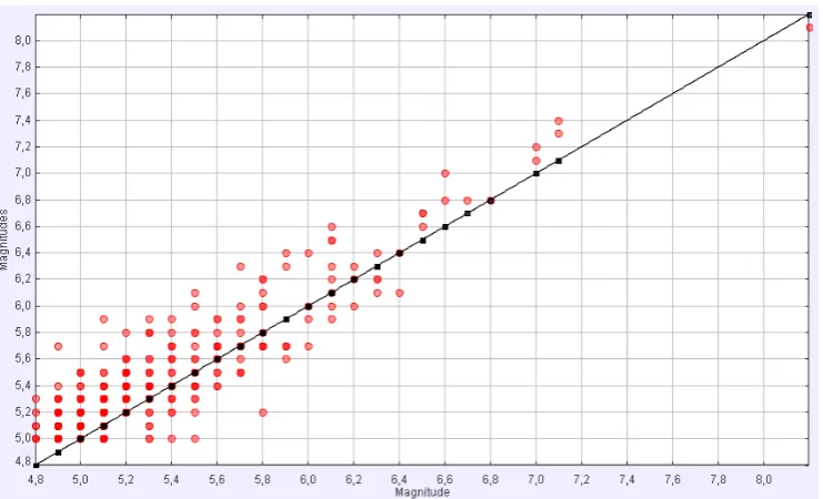
Figure 1. Data comparison of magnitude measurements between BMKG (red full-circles) and the reference straight line provided by the GLOBAL CMT catalog, where earthquake events with the same
magnitudes measured by both institutions are marked as black squares lying on the line.
Physics Page 221
separate graphs for each. Figure 1 describes distribution of eartquake magnitudes for all events issued by BMKG marked as red full-circles in majority and several black squares (as they are lying on the black straight line, which is defined as a reference for magnitude measurements given by the GLOBAL CMT catalog). With the majority of all cases with various magnitudes ranging from 4.8 to 7.1 positioning outside the reference line, we conclude that the measurements of magnitudes performed by the two authorities do not agree well one to another.
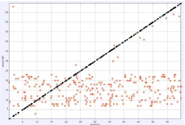
Figure 2 shows origin time data estimated by BMKG in red dots spreading, again, large areas outside a series of other data in black forming a straight line as references provided by the GLOBAL CMT catalog.
Figure 2. Data comparison of origin time measurements between BMKG (red full-circles) and the data series provided by the GLOBAL CMT catalog, where earthquake events that occurred at the same times
observed by both institutions are marked as black squares in the series.
As with magnitude measurements, a large number of red dots are distributed away from the series-formed straight line, and thus the origin time measurements by both institutions are inarguably different. The estimates of origin time in many cases are expected as accurate as possible for a tsunami early warning to reduce disaster risks to minimum. Considering this, the data of origin time for all cases during a period of 4 years from 2012 to 2015 provided by BMKG are not reliable ones.
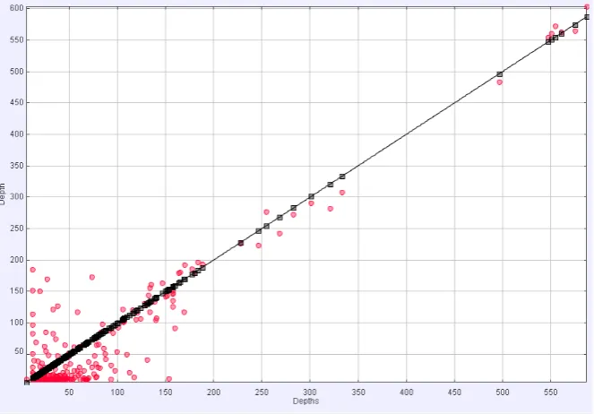
Physics Page 222 Figure 3. Data comparison of depth measurements between BMKG (red full-circles) and the reference line
provided by the GLOBAL CMT catalog, where earthquake events with the same depths measured by both institutions are marked as black squares in the line.
Figure 4. A map of places of interest in this study, showing distribution of epicentres from all cases predicted by BMKG using Ina-TEWS for automatic processing when an event occurs.
Physics Page 223
Among the common parameters, data of epicentres given by BMKG for all events during 2012-2015 are consistent with those provided by the GLOBAL CMT catalog. This is clearly seen in two figures for comparison. Figure 4 shows distribution of epicentres, spanning from the west in northern Sumatra that includes Aceh and westcoast of Sumatra to the east in eastern provinces that include northern parts of Sulawesi, Maluku and Papua, with each location is marked as red dots, which is very much the same pattern given by the GLOBAL CMT catalog marked as green dots in Figure 5. One plausible reason for the coincidence of the above data given by both institutions is that earthquake epicentres are determined by
either seismic stations or satellites using measurements at the Earth’s surface with minimum
disturbed noises relative to measurements of other parameters, such as magnitude, origin time and depth. Keep this in mind, with only one parameter agrees well with the GLOBAL CMT catalog we cannot rely on earthquake analyses using the common parameters usually used by BMKG. For better prediction of potentially tsunamigenic events at various depths and magnitudes as well as better estimates of origin times and epicentres, we need to examine and propose new tsunami parameters. As pointed out by Madlazim (2011; 2013), the need for rapid information of high accuracy is a must for appropriate tsunami assessment in order to minimise false warnings that may lead to fatal decisions concerning with hazard mitigation.
The weakness of the existing methods in determining earthquake magnitudes accurrately and quickly indicates that two main factors required for a tsunami alert triggered by a major earthquake below the sea level are accuracy and rapidness of information. These shortcomings must be then overcome to assess the magnitude of a destructive tsunamigenic earthquake accurately and quickly as they are key solutions to the problem of a reliable tsunami early warning system (Katsumata et al., 2013). If this is achieved, then disaster risk reduction program run in the country particularly victims due to disastrous events, such as earthquakes and tsunamis, can be reduced to a minimum.
4. Conclusions
This study has carefully examined and evaluated the Ina-TEWS performance using common earthquake parameters, including magnitudes, origin times, depths and epicentres of events occurring in a region of the Indonesian archipelago recorded by BMKG during a current period of 2012-2015. The results are then compared with those provided by the GLOBAL CMT catalog. While the first three parameters given by the two institutions have significant differences, the distribution of epicentres for all cases during years considered in this study agrees largely one to another. In short, the Ina-TEWS performance needs to be improved for a better prediction, analysis of tsunamigenic earthquakes and tsunami hazard assessment in terms of both accuracy and rapidness. This finding therefore calls for an alternative method of analyses of tsunamigenic earthquakes that include rapid determination of magnitudes accurately using tsunami parameters other than the present parameters proposed in this study.
Acknowledgements
The authors sincerely thank the Indonesian Agency for Geophysics, Climatology and Meteorology (BMKG) in Jakarta and the GLOBAL CMT for providing full supports of all the necessary data for the work.
References
Physics Page 224
Delouis, B., Charlety, J. & Vallée, M. 2009. A method for rapid determination of moment magnitude Mw for moderate to large earthquakes from the near-field spectra of strong-motion records (MWSYNTH). Bulletin ofSeismological Society of America, Vol. 99, No. 3,pp. 1827-1840.
Dziewonski, A., Chou, T. A. & Woodhouse, J. H. 1981. Determination of earthquake source parameters from waveform data for studies of global and regional seismicity, Journal of Geophysical Research, Vol. 86, pp. 2825-2852.
Ekström, G. 1994. Rapid earthquake analysis utilizes the internet: Computers in Physics, Vol. 8, pp. 632-638.
Katsumata, A., Ueno, H. Aoki, S., Yoshida Y. & Barrientos, S. 2013. Rapid magnitude determination from peak amplitudes at local stations. Earth, Planets and Space, Vol. 65, pp. 843–853.
Kawakatsu, H. 1995. Automated near-realtime CMT inversion. Geophysical Research Letters,Vol.22,doi: 10.1029/95GL02341.
Lomax, A. and A. Michelini, 2009. �Wpd: A duration-amplitude procedure for rapid determination of earthquake magnitude and tsunamigenic potential from P waveforms. Geophysical Journal International, Vol. 176, Iss. 1, pp. 200-214.
Madlazim, 2011. Towards Indonesian tsunami early warning system by using rapid rupture duration calculation. Science of Tsunami Hazards, Vol. 30, No.4.
Madlazim, 2013. Assessment of tsunami generation potential through rapid analysis of seismic parameters – a case study: comparison of earthquakes of 6 April and of 25 October 2010 of Sumatra. Science of Tsunami Hazards, Vol. 32, No. 1.
Physics Page 225 THE ANALYSIS INFILTRATION HORTON MODELS AROUND THE SAGO
BARUK PALM (Arenga microcarpha Becc) FOR SOIL AND WATER CONSERVATION
Marianus1*
1Department of Physics Education , Faculty of Mathematics and Natural Science, State University of Manado,
Minahasa, Indonesia
Abstract
Infiltration is one components of the hydrolocal cycle and very important in conservation of soil and water. Sago baruk palm(Arenga microcarpha Becc) is an endemic plant and used as a source of local food to the citizen in Sangihe Island. This plant also known by locally people as plants to protect soil and water availability.
The aim of this research was to analyze the rate of infiltration and gain empirical equation models infiltration capacity around sago baruk plants in different seasons and different altitude.
The research was conducated at the Gunung village, District of Central Tabukan Sangihe in June to September 2014. Gunung village is spread from the coast to the top of the hill with an altitude of ±600 meters above sea level. Land used is mixed gardens, coconut, cloves nutmeg and Sago. Tools or material used are ; a set of double ring infiltrometer, soil tester, GPS, clinometer and Stopwatch. The method used is survey methods, and techniques of data analysis is descriptive analysis, t-test, and F(ANOVA)-test.
The results of this research showed that the infiltration rate near a cluster of Baruk sago is higher than the outside cluster in the second season, the infiltration rate is higher in the dry season than the wet season. The result Obtained by the model equations infiltration and the constant infiltration capacity around baruk sago plant in accordance with the model standard proposed by Horton and sago baruk plants very suitable for soil and water conservation.
Keywords : Horton model infiltration, conservation, sago baruk
1. Introduction
Physics Page 226
infiltration (Araghi,et all,2010). Vegetated lands generally absorb more water due to organic matter and micro-organisms and plant roots tend to increase soil porosity and stabilize soil structure (Garg, 1979).
Sagu baruk palm is not only used as a source of carbohydrates but it is also valuable for reforestation program (Mahmud and Amrisal, 1991; Samad, 2002). Sagu plant shows highly resistant to the drought. In the long dry season which other crops usually do not survive, the palm still can grow and productize. Sagu baruk palm can grow naturally to form 5 to 6 seedlings every month (personal Communication with sagu baruk farmers, 2014). In cultivating the plant, farmers do not particularly apply a special treatment but just cleaning when they cut down sagu trees from the cluster. Its economic value is one of the advantages of sagu baruk palm. Its ability which holds and distributes water into the soil as well as the ability to grow on dry land is highly reliable potential for utilizing sagu palms as superior carbohydrate plants.
The purpose of this study were to analyze the rate of infiltration and gain empirical equation models infiltration capacity around sago baruk plants in different seasons and different altitude.
2. Materials and Methods
The research was conducted from June to September 2014 at Gunung Village, Tabukan Tengah, Sangihe Island District. The materials of the experiments from mixed farm land with an altitude of ± 600 m above sea level. The tools used for this experiment were GPS, clinometers, set of double ring infiltrometer and stop watch. The altitude in this research was divided into 3 levels, namely high altitude (400-600 m), the medium altitude (200-400 m), and the low altitude (0-200 m) based on the type and soil physical properties. The method of this research was a survey with a purposive sampling method. Data analysis techniques included descriptive analysis, T test and F test (ANOVA) using SPSS 16.00.
The Infiltration rates near the cluster (<0.5 m) and outside the cluster (2.5 m) were calculated using Horton equation model of f t = fc + (fo - fc) e-kt where; ft = infiltration capacity at time t, fc = infiltration capacity when the price reaches a constant value; fo = the value of the initial infiltration capacity (at t = 0); k = a constant that varies according to soil conditions and the factors that determine the infiltration; t = time; and e = 2.71828 (Seyhan, 1977; Garg, 1979).
The rate of infiltration and infiltration constant were obtained using descriptive analysis, which is a table the average value of the infiltration rate and infiltration constant based on season and altitude position. T test at Sig t <0.05 (level of error 5%) was performed to compare values observed in the rainy and dry seasons. Differences in infiltration rates and infiltration constants of the three altitudes (508 m, 330 m and 44 m) were tested using F test or ANOVA at Sig F <0.05 (level of error 5%).
3. Results and Discussion
3.1. Horton Formula Models Around Sagu Baruk Palm
Model equations and the constant infiltration capacity at around baruk sago palms in various soil conditions obtained from the measurement data and calculation of the rate of infiltration. Infiltration capacity equation form as a function of time from the model developed by Horton are:
Physics Page 227
fc = infiltration capacity when the value reaches a constant . fo = the value of the initial infiltration capacity (at t = 0)
k = a constant that varies according to soil conditions and the factors that determine the infiltration. t = time (Seyhan, 1977; Kumar 1979)
e = 2.71828 (the base of natural logarithms)
The results of the equation is as follows
Infiltration equations near the cluster of the rainy season: ft = 0.01 + 6.20 e-0, 463 t
Infiltration equation out cluster of the rainy season: ft = 0.01 + 1.72 e -0.197 t
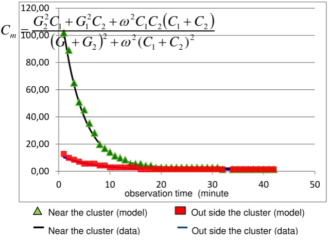
Infiltration equation near the cluster of dry season: ft = 2.23 ++128.45 e-0, 251 t
Infiltration equations outside the cluster during the dry season: ft = 1.24 + 11.06 e - 11.06 t
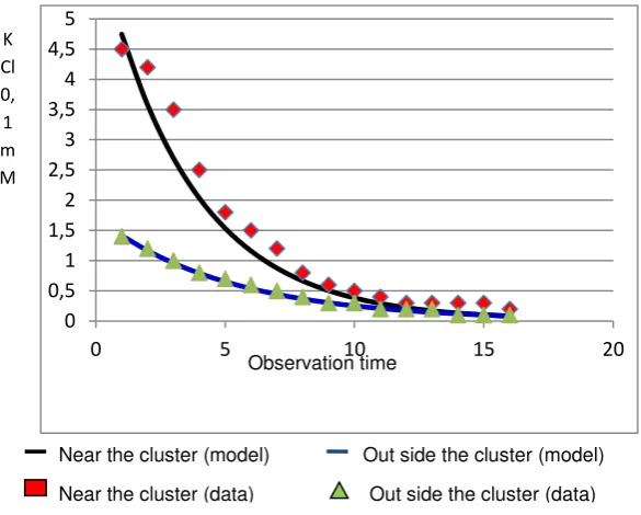
The infiltration capasity curve during the rainy season as shown at figure. 1 below
Figure 1. Infiltration capacity curve during the rainy season
Next the initial infiltration rate is presented comparison, the final infiltration rate, the average infiltration rate, and the constant infiltration in both seasons (dry and wet), and three height positions (top, 508 meters above sea level, the center, 330 meters above sea level, and below 44 meters above sea level), under conditions close to and outside the cluster. Analysis tools used in the observation of the physical condition of the environment around the plant sago baruk are (1) descriptive statistics, (2) t test, and (3) ANOVA test(Suryabrata,1983). In the data presented and the calculation of the rate of infiltration, and the constant infiltration capacity, divided into two seasons, namely dry and rain. There are four variables that were observed in the data measurement and the calculation is the initial infiltration rate (fo), the final infiltration rate (fc), the average infiltration rate (f), and the constant infiltration (k) in both conditions (near the cluster of <0.5 m, and outside the cluster 2.5 m. These variables are presented comparative value of each season.
Physics Page 228
The infiltration capasity curve during the dry season as shown at figure .2 below
Figure 2. Infiltration capacity curve in the dry season
Table 1. Comparison between the infiltration rate of Season
Variable Dry season Rainy season Sig t Remarks
3.2. Analysis of The Results of The Dry Season
Table 2. Comparison between the position of the infiltration rate of the dry season
Variable Position Anova Result
Hight Midle Low Sig F Description
fo near cluster 130.51 130.52 131.02 0.017 Significan
fo out cluster 12.27 12.36 12.26 0.512 Notsignifican
fc near cluster 2.20 2.24 2.24 0.039 Significan
fc out cluster 1.24 1.24 1.24 0.412 Notsignifican
f near cluster 102.57 103.49 102.63 0.242 Notsignifican
Physics Page 229
In this study, the study site is divided into three positions. First, the top position with a height of 508 meters above sea level. Second, the center position with a height of 330 meters above sea level. Third, the down position with a height of 44 meters above sea level. There are four variables that were observed in the data measurement and the calculation is the initial infiltration rate (fo), the final infiltration rate (fc), the average infiltration rate (f), and the constant infiltration (k) in both conditions (near the clump of <0.5 m, and outside the clumps 2.5 m. These variables are presented comparative value of each position in the dry season.
From the above results in the dry season, seen a difference in the initial infiltration rate, the final infiltration rate, and significant infiltration konsntantan between the three positions. Position the top with a height of 508 meters above sea level is characterized by initial infiltration rate is lower, the rate of infiltration of the lower end, and a constant infiltration low position with a height of 330 meters above sea level was characterized by high initial infiltration rate, infiltration rate of the high , and constant infiltration is low. In the low position with a height of 44 meters above sea level is characterized by high initial infiltration rate, and constant infiltration is low.
3.3. Analysis of The Results of The Rainy Season
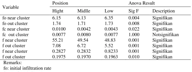
Table 3. Comparison of infiltration rates between the position of the Rainy Season
Variable Position Anova Result
Hight Midlle Low Sig F Description
fo near cluster 6.15 6.13 6.35 0.004 Signifikan
fo out cluster 1.74 1.71 1.73 0.008 Signifikan
fc near cluster 0.0100 0.0042 0.0043 0.022 Signifikan
fc out cluster 0.0077 0.0080 0.0077 1.000 Notsignifikan
Physics Page 230 4. Conclusion
The results of this research showed that the infiltration rate near a cluster of Baruk sago is higher than the outside cluster in the second season, the infiltration rate is higher in the dry season than the wet season. The result Obtained by the model equations infiltration and the constant infiltration capacity around baruk sago plant in accordance with the model standard proposed by Horton and sago baruk plants very suitable for soil and water conservation.
References
Araghi P.F., Mirlatifi S.M., Dashtaki, G.Sh. and Mahdian, M.H. 2010. Evaluating some infiltration models under different soil texture classes and land uses. Iranian Journal of Irrigation and Drainage, 4(2):193-205.
Balai Riset dan Standarisasi Industri Manado. 2006. Enzymatic processes of glucose syrup from Sagu Baruk. Bulletin Palma 93: 10-15. (in Indonesian).
Barri, N. and Allorerung, D. 2001. A survey on plant diversity and habitat ecosystems of Sagu Baruk at Sangihe Talaud Regency. Final Research Report, Indonesian Coconut and Palmae Research Institute. 115 pages (in Indonesian).
Dinas Pertanian Rakyat Propinsi Dati I Sulut. 1980. Various research reports on Sagu Baruk at Pulau Sangihe Besar of Sangihe Talaud Regency. Bulletin Palma 26:21-22. (in Indonesian).
Dinas Pertanian, Perkebunan, Peternakan and Kehutanan Kabupaten Kepulauan Sangihe. 2009. Annual Report. pp 25-30. (in Indonesian).
Garg, S.K. 1979. Water Resources and Hydrology. 3rd edition. Dehli Khanna Publisher, 486 p. Gliessman. S.R. 2000. Agroecoloy: Ecological processes in sustainable agriculture. Lewis
Publishers, Boca Raton-London, New York, Washington, D.C. 357 p.
Kumar, S. 1979. Water Resources and Hydrology. Khanna Publishers, Nai Sarak.New Delhi. p.142-150
Lay, A., Allorerung, D., Amrizal. and Djafar, M. 1998. Sustainable processing of Sagu. Research reports on Coconut and Other Palms. Bulletin Balitka 29: 73-75. (in Indonesian).
Mahmud, Z, and Amrizal. 1991. Palmae for food, feed and conservation. Bulletin Balitka 14:112-114. (in Indonesian).
Rostiwati, T. 1988. Planting techniques of Sagu, Centre for Plantation Forest Research and Development, Bogor. Bulletin Palma.235:13-18. (in Indonesian).
Samad, M.Y. 2002. Improving small scale sagu industry through application of semi mechanical extraction. Indonesian Journal of Science and Technology Vol.4, No.5, hal. 11-17. (in Indonesian).
Seyhan, E. 1977. Fundamental Hydrology. Geografisch Institute der Rijks Universitiet, Utrect. The Netherlands.
Physics Page 231 CHARACTERISTICS OF SUDAN III-POLY(N VINYLCARBAZOLE) COMPOSITE
FILM FOR OPTICAL SENSOR APPLICATION
Heindrich Taunaumang1*, Raindy Xaverius Dumais1, Jinno Pondaag1
1Department of Physics, Faculty of Mathematics and Natural Sciences, State University of Manado,
Minahasa, Indonesia
Abstract
Photo-responsive molecule Sudan III has been developed in form of thin film to pursue their excellent properties especially for optical sensor device application. However, thin film of Sudan III possesses a weak mechanical property. And therefore in order to enhance this functional property of the Sudan III molecule was embedded within polymer matrix to form composite material. In this research, the thin films composite of Sudan III-Poly(N-Vinylcarbazole) or Sudan III/PVK were fabricated by using casting and spin coating methods. The structure of Sudan III-Poly(N-Vinylcarbazole) composite material were characterized by using FTIR, XRD measurement and for the optical property (absorbance) by UV-VIS measurement. In this paper the experiment results are presented.
Keywords : composite material, spin coating, Sudan III, optical property.
1. Introduction
Research on azobenzene based molecules such as DR1, DR19 and Sudan III have been studied. These molecules consists of OH and N=N groups which are responsive to optical field and its environment (others molecules) through molecular interaction such as hydrogen bonding or Van der Walls interaction. The optical property (absorbance) is strongly influenced by the formation (cis-trans) of azobenzene molecules . In this work, composite film of Sudan III/PVK was fabricated for sensor devices application. The gas sensor technology is important for controlling pollution or hazard gas (gas corrosive) such as H2S, CO2 which related to clean environment protection. For sensor technology devices applications the sensitivity, selectivity and responsive time are required and these characteristics are strongly determined by physical and chemical properties of the materials used. Material responsive used in this research is Sudan III. However, thin film of this molecule possesses a weak mechanical property and therefore for sensor technology applications this molecule should be embedded within polymer matrix such as poly (N-vinylcarbazole) or PVK, PMMA.
In this work, the thin film composite of Sudan III/PVK have been fabricated by using casting and spin coating solution methods and this film possesses smooth surfaces, homogenous thickness, and good optical stability. This paper is intended to study the structure and the optical characteristic of Sudan III/PVK composite film which were obtained from the FTIR, XRD and UV-VIS measurement.
2. Material and Method
2.1. Material: Sudan III
Physics Page 232 Figure 1. The molecular structure of Sudan III
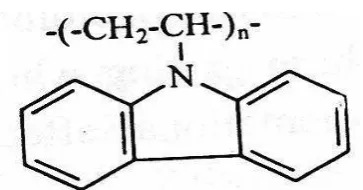
2.2. Material: Poly (N-vinylcarbazole)
Poly(N-vinylcarbazole) or PVK is known as a polymer photoconductive. This molecule has Glass transition 200oC and refractive index no,20 = 1.696. The polymer structure is shown in Figure 2. This polymer was purchased from sigma in form of pellet.
Figure 2. Polymer structure of poly (N-vinylcarbazole)
2.3. Samples Preparation
The solution of Sudan III and PVK samples were prepared by dissolving Sudan III and PVK powder respectively into cloroform as a solvent. The homogeneous solution of Sudan III and PVK were obtained by stiring the solution for about six hour by using a magnetic stirer.
The solutions of Sudan III//PVK were prepared with different composition (% weight ratio) as the following:
a. Sudan III/PVK (1:3) b. Sudan III/PVK (1:4)
The film of PVK and film composite of Sudan III/PVK with 1:3 and 1:4 were prepared by using spin coating method.
2.4. Samples Characterization
2.4.1. FTIR Measurement
In this research the molecular structure are characterized by using FT-IR 801 Single Beam
Spectrophotometer. The measurement was carried out in the “frequencies” (wave number)
range of 4600-400 cm-1. From the FTIR spectra can be identified the molecular structure of the composite material. The absorption spectra indicate the interaction between electromagnetic radiation (IR radiation) and electrical dipole moment.
The absorption peaks (A) in the FTIR spectra are corresponding to an electrical dipole
the following equation (1).
2 2
2
n n
μ μ
A .E E cos θ
r r
Physics Page 233 crystalline order, crystalline orientation and also for estimation of crystalline size material.
The XRD measurement has been carried out by using a diffractometer that based on the reflection method of x-ray radiation. The XRD spectra were performed as diffraction peak intensity corresponding to the diffraction angle. From the spectra of XRD measurement can be determined the planes distance of the crystal (dhkl) according to the Bragg equation (2).
Where h, k and l indicate the lattice plane parameter, indicates x-is diffraction angle. For organic polymer usually using
Cu-of the XRD spectra can be related to the crystalline order or crystal size and also molecules orientation in the film. The width of the XRD spectra (Bhkl) corresponding to the crystal size which is stated by the Scherer formula in equation (3):
Bhkl hkl (3)
hkl
angle, and k is a constant (k=0,89). Sample which has a small crystalline size indicate a wide diffraction peak.
In this experiment the XRD measurement has been carried out in the range of diffraction angle: 10-80o, by using Philips Diffractometer. In this measurement diffraction XRD pattern
Angstrom).
2.4.3. UV-VIS measurement
The optical characteristics of Sudan III molecules and PVK in form of solution and film were obtained from UV-VIS measurement. This measurement was carried out using an instrument of Beckmen DU-7000 Single Beam Spectrophotometer. This measurement obtained UV-VIS spectra in range of 250-800 nm. The background of the sample was first measured. The solvent used for Sudan III and PVK solution samples were chloroform.
(k) according to equation (4).
(4)
Physics Page 234
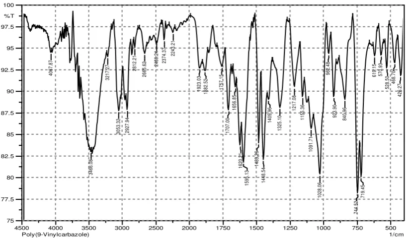
Figure 3. FTIR spectra of Sudan III powder in KBr matrix.
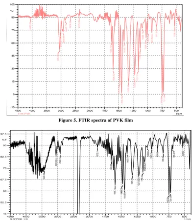
Figure 3 shows the FTIR spectra of Sudan III powder in KBr matrix. Figure 4 shows the FTIR spectra of PVK powder in KBr matrix. Figure 5 shows the FTIR spectra of PVK film. Figure 6 and 7 show the FTIR spectra of composite Sudan III/PVK powder in KBr matrix.
Physics Page 235
Figure 5. FTIR spectra of PVK film
Figure 6. the FTIR spectra of composite Sudan III/PVK (1:3) powder in KBr matrix
Physics Page 236
The N=N stretching in Sudan III/PVK composite powder material is relatively more stronger then for Sudan III which indicates that the Sudan III in polymer matrix is more freely it is mean that the separation between Sudan III molecule within polymer matrix is bit larger. The composite material structure as a combination of both material namely Sudan III and PVK.
3.2. XRD Measurement Results
Figure 8 and 9 show the XRD measurements results of Sudan III/PVK composite film. Figure 8 and 9 are the XRD pattern for Sudan III/PVK composite film. These figure show a wide XRD pattern which indicates that the sample has a small crystalline size or low crystalline order. However for Sudan III (figure 11) powder show sharp XRD pattern which indicates that Sudan III possesses a big crystalline size or high crystalline order. Figure 10 is the XRD pattern of PVK film. This XRD pattern is similarly with figure 8 and 9.
Figure 8. The XRD pattern of PVK film
Figure 9. The XRD pattern of Sudan III pristine powder
22,62 22,6
13,3 24,8
Physics Page 237
Figure 11 show the XRD pattern of Sudan III pristine powder. Figure 12 shows the XRD pattern of PVK powder. The XRD pattern of PVK powder indicates that the crystalline size is small.
Figure 10. The XRD pattern of PVK powder
Figure 11. The Spectra of UV-VIS measurement of solution of (A). PVK in chloroform solvent. (B). Sudan III in chloroform solvent
Figure 12. The Spectra of UV-VIS measurement of (A). Sudan III/PVK composite solution (chloroform solvent ) with composition 1:3. (B). Sudan III/PVK composite solution (chloroform solvent ) with
composition 1:4.
7,7
19,3
72,5
299 nm
345 nm 517 nm A
B
-0,5 0 0,5 1 1,5 2 2,5
0 200 400 600 800 1000
Series1
Series2
299 nm 345 nm
517 nm
A B
-1 0 1 2 3 4 5 6
0 200 400 600 800 1000
Series1
Physics Page 238 3.3. UV-VIS Measurement Results
Figure 13 (A) shows UV-VIS Spectra of of solution of PVK in chloroform solvent and the figure 13 (B) shows UV-VIS Spectra of solution of Sudan IIIin chloroform solvent. The
UV-VIS of Sudan III shows a maximum ab max) at 517 nm, and 345 nm, and 299 nm
corresponding to electronic energy transition of 2.4 eV, and 3,6 eV and 4.2 eV respectively . This spectra exhibits a broad absorption band at 517 nm, with high intensity which indicates
of strong oscillato
-electronic transition through azobenzene.
Figure 13. The Spectra of UV-VIS measurement of (A). Film of Sudan III/PVK composite with composition 1:3 produced by spin coating.(blue line) (B). Film of Sudan III/PVK composite with
composition 1:4 produced by spin coating.(red line)
Figure 13 (A) shows UV-VIS spectra for sample of PVK solution (chloroform) that do not exhibit absorption band in visible region. In other word, the visible region is transparent. However this spectra shows two maximum absorptions in UV region i.e., at 299 nm and 345 nm which corresponding to electronic energy transition of 4.2 eV and 3,6 eV. This spectra exhibits a narrow absorption band with low intensity which indicates of weak oscillator of
-The UV-VIS spectra (figure 15) shows an absorption p = 517
nm and two maximum absorption in UU- 3 = 299 nm which
corresponding to electronic energy transition of E1 = 2.4 eV and E2 = 3,6 eV, and E3 = 4.2 eV respectively. The figure do not shows a significant shifting in absorption peak to the longer wavelength (red-shift) or shifting to the shorter wavelength (blue-shift). The film of composite of Sudan III/PVK with composition 1:4 shows lower intensity and narrow absorption band in the visible region compared to the Sudan III/PVK with composition 1:3. The differences of absorption band form due to electronics transition contribution of Sudan III molecules in the composite. The UV-VIS spectra film Sudan III/PVK clearly shows absorption peak in the visible region and this potentially to be developed as optically sensor. The UV-VIS spectra film of Sudan III/PVK composites shows that the optical properties of the composites as combination of its optical properties components i.e., Sudan III and PVK.
4. Conclusions
Physics Page 239
polymer matrix is more freely it is mean that the separation between Sudan III molecule within polymer matrix is bit larger.
The Sudan III/PVK composite film show a wide XRD pattern which indicates that the sample has a small crystalline size or low crystalline order. However for Sudan III powder show sharp XRD pattern which indicates that Sudan III possesses a big crystalline size or high crystalline order.
The optical characteristic especially in absorbance intensity for UV region (345 nm) of Sudan III/PVK composite in form of solution is significantly different compared to the film composite. However, in visible region is relatively stable.
This UV-VIS measurement indicates that the film of Sudan III/PVK can be potentially to be developed for optical sensor application.
Acknowledgments
Thank for DP2M DIKTI (Directorate High Education of Indonesia) for funding this research By Grant of Hibah Bersaing with letter of agreement No: 31/SP2H/PL/Dit.Litabmas/IV/2011, April 14,2011 and No.2772/UN41/023.04.08/2012, September 20, 2012.
References
Alkins, E. (1974), X-Ray Structure Determination of Polymers, In Electronic structure of Polymers and Molecular Crystals, Edited by J-M. Andre, J. Ladik, J. Delhalle, Plenum Press, New York, 199-226.
Colthup, N.B., L.H. Dally, S.E. Wiberly. (1975), Introduction to Infrared and Raman Spectroscopy, Academic Press, London.
Gede, U.W. (1995), Polymer Physics, Chapman & Hall, London
Ho, M-S., A. Natanshon, and P. Rochon.1996, Azo Polymers for Reversible Optical Storage.9, Copolymers Containing Two Types of Azobenzene Side Groups, Macromolecules.29, 44-49.
Kersey , A.D, A Review of Recent Developments in Fiber Optic Sensor Technology, 1996, Optical Fiber Technology, 2, 291–317.
Kim R. Rogers’, Edward J. Poziomek’, (1λλ6), Fiber Optic Sensors For Environmental
Monitoring, Chemosphere. Vol. 33, No. 6. pp. 1151-l174.
Luo, J, Jinggui Qin, Hu Kang, and Chend Ye, A Postfunctionlization Strategy To Develop PVK-Besed Nonlinear Optical Polymers with a High Density of Chromophore and Improved Processibility, Chem. Mater., 2011,13, 927-931.
Meng, X., A. Natanshon, C. Barret, and P. Rochon. 1996, Azopolymer for Reversible Optical Storage.10. Cooperative Motion of Polar Side Groups in Amorphous Polymers, Macromolecules, 29, 946-952.
Parry D.A, M.Mat Sallah,L.S.Miller, I.R. Peterson, and R.Hollyoak, Investigation Into The Respons of an Optical Gas Sensor Based On Polymeric LB Films, 1997, Supramolecular Science ,427-435.
Physics Page 240
Silverstein, R.W., G.C. Bassler. (1967), Spectrometer Identification of Organic Compounds, Second Edition, John Willey & Sons, Inc. USA, 148-169.
Taawoeda D, H. Taunaumang (2009). Pengembangan Material Fotorefraktif Untuk Aplikasi Fotonik, Laporan Hasil Penelitian Hibah Bersaing, Dibiayai oleh DP2M Ditjen Dikti Depdiknas.
Taunaumang H., D. Taawoeda, (2007). Efek Permukaan dan Suhu Substrat Pada Orientasi Molekul dan Momen Dipol Film Tipis Hasil Deposisi Vakum Dari Molekul Berbasis Azobenzene, Laporan Hasil Penelitian Fundamental, Dibiayai oleh DP2M Ditjen Dikti Depdiknas.
Taunaumang H., Wenas DR, D. Taawoeda, (2008). Pengembangan Material Fotorefraktif Untuk Aplikasi Fotonik, Laporan Hasil Penelitian Hibah Bersaing, Dibiayai oleh DP2M Ditjen Dikti Depdiknas.
Taunaumang H.,D. Taawoeda (2011), Pengembangan Film Tipis Komposit DR19/PVK Untuk
Aplikasi Sensor Optik, Laporan Hasil Penelitian Hibah Bersaing, Dibiayai oleh DP2M Ditjen Dikti Depdiknas. [5]. Taunaumang H, (2012), Fabrikasi dan Karakerisasi Film Tipis Komposit Sudan III/PVK. Laporan Hasil Penelitian Hibah Bersaing, Dibiayai oleh DP2M Ditjen Dikti Depdiknas.
Physics Page 241 THE METHOD AND APPLICATION OF PARAMETER: “THE DIURNAL DYNAMIC AREA OF MICROCLIMATE GRADIENT” IN FOREST ECOSYSTEM
Christophil S. Medellu1*
1Departement of Physics, Faculty of Mathematics and Natural Sciences, State University of Manado,
Minahasa, Indonesia
Abstract
Interaction between forest ecosystem with the adjacent environment, among others described by the parameters: the maximum difference of microclimate variable values, the depth of edge effects and maximum values of edge gradient. In 2012, the author through the dissertation introduces a new parameter that was the area and index of diurnal dynamics of microclimate gradient at the edge of mangrove forests. Parameters of area and index of diurnal dynamics of microclimate gradient include the parameters used by the previous experts. This parameter can characterize the mangrove forest and classify the mangrove ecosystem based on microclimate variables interaction between ecosystem and the adjacent environment. This parameter can be used to monitor and analyze the ecosystem and the adjacent environment changes. This article describes the method and application of parameter: area and index of diurnal dynamic of microclimate gradient in characterization of forest and forest interaction with the environment.
Keyword: microclimate variables, edge gradient, area, index, diurnal dynamic.
1. Introduction
Microclimate variables used in the study of forest ecosystems because it is sensitive to variations in the ecosystem as well as changes in the ecosystem and adjacent environment (Morrisey et al., 2007; Gradstein, 2008). Daily changes of microclimate around the edge of the forest, reflects the thermal energy difference between the forest ecosystem and the environment (Potter et al., 2001; Spittlehouse et al., 2004). Changes in forest structure due to natural factors or human activities, detected through the changes of temporal and spatial variations of microclimate variables (Brosofske et al., 1997; Nelson et al., 2007). Fragmented forests show the higher microclimate fluctuations than homogenous forests (Ma et al., 2010). Microclimate around the patches or forest boundaries, were more fluctuated than the central of forest (Medellu, 2012). This relates to the irradiation and thermal energy transfer between the ecosystem components and the environment.
Physics Page 242
temperature in characterizing the ecosystem of dalugha (Cyrtosperma merkusii (Hassk.) Schott)
Besides to vary in variables, the characterization of the ecosystem also varies in the using of parameters. The area was widely studied to characterize forest ecosystems is edge of forest. Microclimate variables in the edge or in the forest boundaries, fluctuates more than in the central of forest (Heithecker and Halpern, 2007, Davies-Colley et al., 2000; Zheng et al., 2000). Forest edge is an area around the limits of forest ecosystems or the limit of forest fragmentation and patches (Medellu, 2012). Parameters are widely used by researchers to describe the daily changes of microclimate around the edge of the forest were the edge gradient (Rambo and North, 2008; Chen et al. 1995; Williams-Linera et al. 1998; Gehlhausen et al. 2000; Newmark 2001; Cienciala et al. 2002), and the depth of edge effects (Gehlhausen et al. 2000; Stewart and Mallik, 2006; Medellu et al., 2012; Ibanez et al., 2012). Edge gradient and depth of edge effect change throughout the day as a result of the irradiation and thermal energy transfer between the environment and forest ecosystems (Medellu, 2012; Ibanez, 2012).
In 2012, the authors formulate a new parameter that was the edge gradient diurnal dynamic area, for characterization of mangrove forests. The edge gradient diurnal dynamic area is the area between the curves of diurnal edge gradient with a line of thermal equilibrium between forest and environment. Thermal equilibrium line is a horizontal line in coordinate system of the time versus gradient. Thermal equilibrium line has a value of zero edge gradient, and demonstrates the condition that no flow of energy between the forest and environment (Medellu, 2012). This paper discus the method and application of parameter: edge gradient diurnal dynamic area in characterizing the mangrove ecosystems. Microclimate variables discussed here are the air temperature and humidity.
2. Determination of Diurnal Dynamic Area of Microclimate Gradient
Mathematical model of the edge gradient diurnal dynamic area (Medellu, 2012; 2013) is:
A =∑��=� ��.�………..………(1)
Δt is the sampling interval of time as the dependent variable and Gi is the value of edge gradient of sample i in the time interval of t1 – t2. T1 and t2 indicates the time of the first and second thermal equilibrium between forest ecosystems and the environment. The procedure for determine the edge gradient diurnal dynamic area was as follow:
2.1. Determination of Fourier Function of Microclimate Variables
T t = T + ∑�/�= amcos ωmt + bmsin ωmt………..…(2)
where
ω
m= 2πm/N
……….………..(3)………....………(4a)
Physics Page 243
T(t) is the Fourier function, m is the harmonic number of Fourier series, N is the number of data pairs of independent (t) and dependent (f(t)) variables. Daily measurement of microclimate variable with one hour internal, produce data pairs N = 24. T0 is the average of dependent variable values. Mathematical procedure for Fourier function formulation of each point of measurement along the transect (Medellu, 2012, 2013) is:
a. Determination of Fourier coefficient am and bm, using equation (4b) and (4c). b. Determination of coefficient cm using the relation cm2 = am2 + bm2.
c. Determination of diversity coefficient : sm = (cm2/(2.σ))*100
σ is the standard deviation of microclimate data. Through these steps we found am, bm, cm and sm data, for m = 1, 2, …..12. Diversity coefficient (sm), determine the number of harmonic to construct the Fourier function model with define degree of accuracy. Higher number of harmonic means higher number of Fourier series, guaranties the high precision of function.
Figure 1 presents the Fourier function graphics of air temperature at the position of 1 m outside the forest, at the edge and at position 16 m to the central of mangrove forest in Talengen bay. Figure 2 presents Fourier function graphics of humidity for the same transect and positions.
Fourier function of air temperature at the edge of mangrove (x=0), transect no.2 – Talengen bay is:
T(t) = 29.3720 - 1.3072.cos(πt)/12 + 5.5511.sin(πt)/12 - 1.015λ.cos(πt)/6 - 0.3812.sin(πt)/6 +
0.0λλ.cos(πt)/4 - 0.137.sin(πt)/4 + 0.225.cos(πt)/3 - 0.040.sin(πt)/3 (0C)
and the Fourier function of humidity at the edge of mangrove, transect -2, Talengen Bay is
H(t) = 74.608 + 3.280.cos(πt)/12 - 13.703.sin(πt)/12 + 1.323.cos(πt)/6 + 0.352.sin(πt)/6 -
0.076.cos(πt)/4 - 0.086.sin(πt)/4 - 0.640.cos(πt)/3 - 0.081.sin(πt)/3 (%)
The degree of accuracy of each functions are 99.3 percent and 99.185 percent (Medellu, 2012, 2013).
2.2. Data Synchronization
Data synchronization needed for not simultaneous measuring between positions along transect. The difference in time of measuring for subsequent positions, are followed by the
Figure-1. Diurnal changes of air tempera- ture at: 1 m out of mangrove ( ), the
Physics Page 244
change of microclimate variable magnitude. Without synchronization, time based spatial function modeling will be bias due to the change of variable magnitude during that time difference. Data synchronization is done by entering time difference data to the temporal function or Fourier function and then we got the corrected time based data. This procedure included in our software.
2.3. Determination of Spatial Function
Mathematical model of spatial function is:
F x = k + k ek − k x ……….…(3)
x is the distance from the edge to the center of mangrove. The constants k1, k2, k3 and k4 obtained by iteration techniques. Usually it takes four pairs of data (x,T), but if it select the reference point data (x = 0), then the constants and coefficients can be determined using three pairs of data, e.g. : (0, T0), (x1, T1), and (x2, T2) (Medellu, 2012, 2013). Procedure of
Spatial function graphics for air temperature and humidity presents in Figure-3 and Figure-4
Spatial function of air temperature at 12.00, for transect no-2 – Talengen bay is: T(x) = 32.99674 + 0.18068.� . − . .x (0C)
and the spatial function of humidity at 12.00 for transect no.2 is:
H(x) = 65.22828 - 775.01073.�− . − . .x (%)
2.4. Determination of Edge Gradient
Figure-3 and Figure-4 shows that the spatial function changes over time as a result of the irradiation and thermal energy transfer processes in forest ecosystems and the environment.
Figure-3. Spatial function of air
Physics Page 245
Mathematically, this spatial function change means the changes of the spatial gradient at the edge of forest. Gradient of spatial function at the edge of forest determined using formula: G = dF(x)/dx for x = 0 (Medellu, 2012, 2013), or
G = - k2.k3.exp ( k3 ) ...(4) The constants k2 and k3 change over time, so that G is time dependent or daily dynamic. Figure-3 and Figure-4 shows the change of slope and gradient direction, that represents the direction and intensity of thermal diffusion across the forest edge (Medellu, 2012).
2.5. Determination of Edge Gradient Diurnal Dynamic Area
Diurnal dynamics of microclimate gradient function at the forest edge is the Fourier function. This function determined by the same procedure with procedure of the point-1. Figure 5 and Figure 6 are the graphics of the daily dynamics of the edge gradient of air temperature and humidity on a transect-2, in Talengen bay.
Fourier functions of edge gradient diurnal dynamic of air temperature and humidity:
T(t) = - 0.2944 - 0.2822 cos(2πt)/12 - 0.7046 sin(2πt)/12 + 0.0246 cos(4πt)/12 +
0.1561 sin(4πt)/12 + 0.1218 cos(6πt)/12 + 0.1218 sin(6πt)/12 + 0.1424 cos(8πt)/12 -
0.1072 sin(8πt)/12 + 0.2327 cos(10πt)/12 + 0.0164 sin(10πt)/12 + 0.202λ cos(πt) -
0.0λ77 sin(πt) ………..
The accuracy of each function for first six harmonic was 95.9 percent and 96.86 percent.
2.6. Determine the Area and Index of Edge Gradient Diurnal Dynamic
The area of edge gradient diurnal dynamic is the area surrounded by the diurnal dynamic gradient curve above and below the thermal equilibrium line (red line, Figure 5 and 6). For air temperature, the area above the equilibrium line represents the area of edge gradient at night, while the area below the equilibrium line represents the day edge gradient. For humidity variable, the area above the equilibrium represents the day and below represents the
Figure-5. Graphic of diurnal dynamic of air temperature at the edge of mangrove, transect-2, Talengen Bay. Source: Medellu, 2012
07.00 11.00 16.00 21.00 02.00 07.00
Figure-6. Graphic of diurnal dynamic of humidity at the edge of mangrove, transect-2, Talengen Bay. Source: Medellu, 2012
Physics Page 246
night. The area of edge gradient diurnal dynamic determined using the numeric integral
method, with sampling interval of time Δt about 0.1 minute. The number of data obtained by
dividing the area above and below the equilibrium line by Δt. Using equation (1) we get the
day and night area of edge gradient diurnal dynamic. The unit of edge gradient diurnal dynamics area is the multiplication of gradient unit with time unit. The unit of edge gradient diurnal dynamics area for temperature is oC.hour/meter, while the unit for humidity variable is: %.hour/meter. Microclimate edge gradient diurnal dynamics index is a quantity of night divided by day area. This index is no unit. The procedure of determining the edge gradient diurnal dynamic area, include other parameters, such as the maximum difference of microclimate variable inside and outside the forest, the maximum edge gradient, and the depth of edge effects. The excess of parameter: edge gradient diurnal dynamic area, is able to demonstrate the energy accumulated in forest ecosystems as well as the transfer of energy between forests and the environment during one day. This parameter can be used to characterize forest ecosystems and to monitor changes in ecosystems and ecosystem-environment interactions (Medellu, 2012).
3. Application of Parameter: Edge Gradient Diurnal Dynamic Area
Summary of mangrove characterization using the software of edge gradient diurnal dynamic area is presented in Table-1. Table-1 shows that the edge gradient diurnal dynamics area of microclimate variables are depends on: (1) the density of canopy cover that associated with the type and condition of mangrove, (2) the environmental as: sea, paved roads, coastal vegetated and not vegetated, (3) any fragments (patches) or open spaces in the mangrove forest. These results verify that this parameter can characterize ecotypes, structure and the adjacent environment condition of mangrove ecosystem. This parameter is also potential to be used as an indicator of changes in forest ecosystems (deforestation, reforestation or trees growth) and the changes in adjacent environment (deforestation, planting, global warming etc.).
Physics Page 247 Tabel-1. Karakteristik transek dan besaran luas bidang dinamika harian gradient suhu udara dan
kelembaban
Figure-7. Transects grouping based on day gradient dynamic area of temperature vs humidity (Medellu, 2013)
8
10
2
5
1
Area of day gradient of temperature (oC.hour/m)