ANALYSIS
Comparison of contingent valuation and conjoint analysis in
ecosystem management
T.H. Stevens
a,*, R. Belkner
a, D. Dennis
c, D. Kittredge
b, C. Willis
aaDepartment of Resource Economics,226Draper Hall,Uni6ersity of Massachusetts,Amherst,MA01002,USA bDepartment of Forestry and Wildlife Management,Uni6ersity of Massachusetts,Amherst,MA,01002,USA
cUSDA Forest Ser6ice,Northeast Forest Experiment Station,Burlington,VT,USA Received 9 July 1998; accepted 18 May 1999
Abstract
Contingent valuation (CV) and conjoint analysis were used to estimate landowner’s willingness to pay (WTP) for ecosystem management on non-industrial private forest land. The results suggest that even when conjoint and CV questions are the same, except for rating and pricing format, respectively, WTP estimates are quite different. Since most conjoint models essentially count ‘maybe’ responses to valuation questions as ‘yes’ responses, we conclude that conjoint model results often produce WTP estimates that are biased upwards. © 2000 Elsevier Science B.V. All rights reserved.
Keywords:Economic value; Contingent valuation; Ecosystem management; Conjoint analysis
www.elsevier.com/locate/ecolecon
1. Introduction
Contingent valuation (CV) is widely used for valuing environmental programs, but this ap-proach is often viewed with scepticism. However, as noted by Boxall et al. (1996), there are alterna-tives; CV should be viewed as only one of several ‘stated preference’ elicitation methods. Other mem-bers of this class include conjoint analysis,
contin-gent choice, and polychotomous choice. Although very few comparisons of these techniques have been published, most empirical comparisons suggest substantial differences (Desvouges and Smith, 1983; Brown, 1984; Magat et al., 1988; Irwin, et al., 1993; Ready et al., 1995; Boxall et al., 1996). For example, Boxall et al. reported CV estimates of willingness to pay (WTP) for moose hunting 20 times higher than those derived from the contingent choice method. On the other hand, Magat et al. (1988) estimated contingent values for risk reduc-tion that were 58% lower than those obtained from a paired comparison choice approach.
* Corresponding author. Tel.: +1-413-5455714; fax: + 1-413-5455853.
E-mail address:[email protected] (T.H. Stevens)
Additional research comparing CV with other types of stated preference techniques is obviously needed. This paper compares CV and conjoint (CJ) techniques in a case study of WTP for ecosystem management of non-industrial private forest land in the Northeastern US.
2. Background and previous research
We are aware of very few studies comparing CV with other types of stated preference tech-niques. With the exception of Boxall et al. (1996), the empirical evidence suggests that WTP esti-mates derived from CJ (or choice) studies are significantly larger than those obtained from the CV method. For example. Barrett et al. (1996) concluded that CJ WTP estimates for two types of water purification programs were four to five times larger than the corresponding CV estimates. Desvouges and Smith (1983) compared CV and contingent rankings for water quality in the Monogahela River. Mean water use values derived from the direct CV question were three to four times less than the values estimated from the rankings approach.
Magat et al. (1988) used a paired comparison approach and an open-ended CV format to derive consumers’ WTP for risk reduction associated with a set of market goods (bleach and drain openers) that differ only in terms of purchase price and risk of injury. In contrast to the one-step open ended CV procedure, the choice method asked each subject to make a series of compari-sons between products in a manner which simu-lated actual choices in the marketplace. The CV approach produced monetary valuations that were 58% lower than the average choice valua-tion. Magat et al. (1988) argue that the CV ap-proach creates incentives for respondents to understate their true value while the choice method eliminates this incentive thereby produc-ing more accurate WTP estimates. However, Box-all et al. (1996) found that CV estimates of environmental quality changes affecting moose habitat were significantly larger than estimates derived from choice experiments.
Although there are many reasons why values derived from CV and other stated preference methods might differ, we focus here on factors specifically related to a comparison of CV and CJ analysis. First, substitutes are made explicit in the CJ format and this may encourage respondents to explore their preferences and tradeoffs in more detail. Indeed, as noted by Gan and Luzar (1993), conjoint analysis ‘can be characterized as an ex-tension of the referendum closed-end CV method in which large numbers of attributes and levels can be included in the analysis without over-whelming the respondents’ (p. 37). As shown by Boxall et al. (1996), when compared to CJ, CV results may therefore be biased upward because respondents to the ‘typical’ CV survey are usually asked to consider fewer substitutes.
Another factor is that from a psychological perspective, the process of making choices in the CJ format may be quite different from that asso-ciated with making decisions about WTP (Irwin et al., 1993; McKenzie, 1993). That is, respondents may react differently when choosing among com-modities that have an assigned price as compared to making dollar valuations of the same commod-ities. Moreover, Irwin et al. (1993) found that WTP questions lead to relatively greater prefer-ence for improved commodities, such as TVs and VCRs, while choice questions yielded relatively greater preference for environmental amenities like air quality. Similar results were reported by Brown (1984). Irwin et al. (1993) concluded that if monetary prices are an attribute, they carry more weight in determining a response measured in dollars (e.g. WTP) than they do in determining a rating or choice response. This arises from the fact that choices are driven from reason and arguments to a greater extent than are pricing responses.
choice format. Their CV question asked respon-dents to determine whether or not they preferred a given program while the polychotomous choice format gave six options (i.e. definitely prefer, probably prefer, maybe prefer, maybe not prefer, probably not prefer, definitely not prefer). This format was motivated by the belief that respon-dents might be more comfortable answering valu-ation questions when given the opportunity to express strength of conviction; since the poly-chotomous method allows for a range of answers, it might produce a more accurate description of respondents’ preferences. In two empirical studies, preservation of wetlands and horse farms, the polychotomous format yielded a higher rate of usable responses and much higher WTP estimates. More recently, Champ et al. (1997) found that although contingent values were greater than ac-tual donations for an environmental good, when the contingent values were restricted to respon-dents who said they were very certain to con-tribute, mean CV and actual donations were not statistically different. Elkstrand and Loomis (1997), Alberini et al. (1997) and Wang (1997) also found that contingent value estimates vary widely depending on how respondent uncertainty is incorporated in the analysis.
3. Theoretical considerations
From the perspective of neo-classical economic theory, the CV and CJ techniques should produce similar results, provided that the CV and CJ formats are properly specified. Suppose that indi-vidual utility associated with environmental qual-ity, EQ, can be expressed as a function of income, Y, and EQ attributes such as water quality, wildlife habitat preserved, and cost. In dichoto-mous choice CV, individuals are asked to under-take activities on their own property to improve EQ that cost them a predetermined amount, $N. The value of utility, observed by the researcher, when amount Nis paid is:
U1=U(D1,Y−N)+e1 (1)
where D1 is a vector of EQ attributes and e is a random variable. Utility when $Nis not paid is:
U0=U(D0,Y)+e0 (2)
where D0 represents EQ attributes for the status quo situation. The individual is assumed to pay if, and only if:
U1]U0 (3)
Utility difference, dV, can be expressed as:
dV=U1−U0 (4)
If utility is assumed to be linear, additive, and separable with respect to income and EQ at-tributes, dV is given by:
dV=U(D1,Y−N)−U(D0,Y)+e1−e0 (5)
The WTP probability can then be written as:
Pr=G(dV) (6)
where G is the probability function for the ran-dom component of utility (e1−e0). Assuming a logit probability function for G, the WTP proba-bility is:
Pr=(1+e−dV)−1 (7)
Median WTP for the EQ improvement, D1−D0, can then be estimated by calculating the value of N, N*, for which dV=0, i.e. at the point of indifference there is a 50% chance that the indi-vidual would pay amount N*.
Following Roe et al. (1996) a CJ format which is conceptually consistent with the dichotomous choice CV format (Eq. (7)) can be derived by asking individuals to rate the current situation without the EQ program as given by (Eq. (2)) and a set of EQ programs, (Eq. (1)). It is implicitly assumed that:
R1=h(U1), andR0=h(U0) (8)
whereR1, andR0are individual ratings andhis a transformation function. Utility difference, dV, is then approximated by the ratings differenceR1−
R0:
dV=R1−R0=U(D1,Y−N)−U(D0,Y)+e1
−e0 (9)
In other words, setting aside the issue of substi-tutes and respondent uncertainty for the moment, if individuals are asked, for example, to rate the status-quo, and programs which cost $N on a scale of 1 to 10 (10 indicating programs they would definitely undertake), a binary response CJ model is obtained which is identical to the di-chotomous choice CV model (Eq. (7)) given the approximation in Eq. (9).
It is important to note that the CJ model set forth in Eqs. (8) and (9) differs from the tradi-tional CJ format in that the dependent variable in Eq. (9) is the ratings difference from the status quo and independent variables are changes in program attributes from the status quo.1
As shown by Roe et al. (1996), this specification provides estimates of Hicksian surplus which can then be directly compared with CV estimates (also see McKenzie, 1990; Johnson et al., 1995).2
However, in empirical applications CV respon-dents are typically presented with far fewer substi-tutes than are CJ respondents. Boxall et al. (1996)
found that CV respondents therefore tend to ig-nore substitutes, and if this difference is not taken into account, choice and CV estimates are very dissimilar. Consequently, comparisons of the CV and CJ techniques requires that: (a) both formats convey the same information about substitutes; (b) the CJ model is specified as outlined in Eqs. (8) and (9); and (c) respondent uncertainty is accounted for.
3.1. Case study
Our comparison of the CV and CJ methods is based on a case study of the willingness of non-in-dustrial private forest landowners to pay for ac-tivities that are compatible with ecosystem management (EM). EM is often defined as ecolog-ically based, sustainable management that blends environmental, social, and economic values (Stan-ley, 1995). Effective EM requires planning on broad spatial and temporal scales, often by defini-tion beyond the bounds of individual private ownership. And, instead of focusing on commod-ity outputs, the EM approach seeks to achieve desired future conditions, with outputs such as timber harvests, wildlife, and recreational oppor-tunities occurring throughout the process (Stan-ley, 1995).
The EM paradigm seeks to manage land in greater synchronicity with the natural patterns and effects of disturbance, habitat, and nutrient and hydrologic cycling. Consequently, adoption of this approach or paradigm by landowners re-quires consideration of their individual property at broader spatial and temporal scales. Approxi-mately 58% of forest land in the United States is owned by non-industrial, private individuals or families. However, as noted by Brunson et al. (1996), very little is known about landowner atti-tudes and preferences related to EM alternatives. Since by definition EM is a broad approach or paradigm, in order to test landowners’ attitudes, it was necessary to create a particular, reasonable situation or case study typical of adopting this approach.
Information about WTP for EM was obtained through a mail survey of all 1116 Massachusetts landowners enrolled in the Forest Stewardship 1The traditional conjoint model involves estimating the
following relationship between ratings and program attributes: Ui=Ri=V(ZK)+Pz=b0Pz+blZ11+...bnZn1+ei (a)
whereUiis individuali’s utility for an attribute bundle;Riis
the individual’s rating,V(·) is the non-stochastic component of the utility function,ZKis a vector of attribute levels,P
zis the price for the attribute bundleZ, andbis the marginal utility or weight associated with each attribute (Johnson et al., 1995). Setting the total differential of Eq. (a) to the point of indifference and solving:
dUi=b0dPz+b1dZ11+…=0 (b) yields marginal rates of substitution for the attributes Z11. Since a price attribute,Pz, is included, the marginal utilities of all attributes can be rescaled into dollars, and marginal will-ingness to pay for each attribute may be derived:
dPz= −b1dZ11/b0or (c) dPz/dZ11= −b1/b0
Program. This program is a voluntary, federally funded program that entitles participants to share the cost of improving their forest land with the federal government. Consequently, survey partici-pants were generally knowledgeable about forest land management activities, and all had 10-year management plans for their properties, prepared by professional foresters.
Landowners were partitioned into two groups. One group received a CV format containing EM management alternatives based on our specific scenario; the second group was given a CJ for-mat. In contrast to the study by Boxall et al. (1996), the CV and CJ questions were virtually identical so that any differences related to substi-tutes would be eliminated. An example of each format is presented in the Appendix.
All respondents were asked to value (rate) the status quo (do nothing) and three EM alterna-tives which involved setting aside a portion of their land to create a buffer zone that would provide a wildlife corridor connecting two larger wildlife habitats; a state forest and town conser-vation land. Respondents were told that the buffer zone would also improve water quality downstream to maintain a wood turtle popula-tion located on the town conservapopula-tion land (see Appendix). The wood turtle, Clemmys insculpta, is listed as a species of special concern in Massa-chusetts.
Each EM option consisted of three attributes; acreage set aside for the buffer zone, increase in wood turtle population, and annual improvement and maintenance costs associated with the buffer zone. There were three possible values for buffer zone acreage, 5, 10, or 20 acres, three levels of increase in the wood turtle population, 0%, 10%, and 25%, and three annual cost levels, $50, $100, and $200. All possible combinations of these were generated and three EM programs, plus the status quo, were randomly assigned to each re-spondent. It is important to note that all possible combinations of EQ program attributes must be considered in order to evaluate interactions be-tween attributes. However, this means that some programs are either redundant or seem inconsis-tent (McKenzie, 1990). For example, program D in Appendix A has less acreage in buffers than
alternatives A and B, yet it has a greater increase in wood turtle population. Consequently, we would expect that program D would receive a higher rating than either A or B, all else held constant.
CJ respondents were asked to rate the three EM options and the status quo on a scale of 1 to 10, with 10 indicating EM programs, if any, the respondent would definitelyundertake and 1 indi-cating that the respondent would definitely not undertake the program. If respondents were not sure, they were asked to use a scale of 2 through 9 to indicate how likely they would be to under-take each EM program. A dichotomous choice CV format was used wherein each respondent was asked whether they would definitely under-take each program (see Appendix B). The 1116 landowners were randomly divided into two groups — 558 CV surveys and 558 CJ surveys were mailed.3
4. Results
The CV response rate was 67% and 42% of the CV surveys returned were fully completed. The CJ response rate was 56%, but 67% were com-pleted giving the CJ format a higher comcom-pleted return rate. It is interesting to note that only 7% of those who returned a CV survey would not pay some amount for an EM program and only 8% of the CJ respondents rated EM programs below the mean status quo rating.
Empirical comparison of the CV and CJ for-mats involved estimating dV (see Eq. (9)). The following approximation of utility difference, dV, was used:
dV=a+b(D)+c(N)+d(F)+e (10)
where D is a vector of EM attributes (acres, turtles), N is the predetermined program cost, F is a set of taste and preference variables which
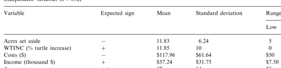
Table 1
Independent variables (n=692)
Mean Expected sign
Variable Standard deviation Range
High Low
6.24 5
Acres set aside − 11.83 20
11.85 10 0
WTINC (% turtle increase) + 25
$200 $50
$117.96
− $61.64
Costs ($)
$31.75 $7.50 $102.50
Income (thousand $) + $57.24
99 25
Age +/− 57 14
1 0
Environment + 0.1299 0.34
differ among individuals, and a, b, c, and d are estimated coefficients.4
Four different econometric models were esti-mated; a dichotomous choice CV logit model (Eq. (7)), two CJ logit models, (Eq. (7)), and a ‘ratings difference’ CJ model (Eq. (9)). The dependent variable in the first CJ model, CJ1, equals 1 if the respondent would definitely undertake an EM program (rating equal to 10), and 0 otherwise. Sensitivity to respondent uncertainty was exam-ined in the second and third CJ models. The dependent variable in the second CJ model, CJ2, equals 1 if the respondent rated an EM program greater than the status quo and 0 otherwise. The third CJ model, CJ3, is a more traditional specifi-cation wherein Eq. (10) is estimated using the Tobit procedure. As shown by Roe et al. (1996), WTP is derived from CJ3 by increasing the value of N until the point of indifference is reached (dV=0).
Independent variables are presented in Table 1. The first variable, acres, is the amount of land respondents were asked to set aside for the pur-pose of EM. We expect a negative relationship between acres and probability of EM program acceptance, all else held constant. The second variable, WTINC, is the percentage increase in the wood turtle population as a result of EM. A positive relationship between WTINC, WTP and program rating is expected. The cost variable is
the monetary commitment incurred by respon-dents undertaking EM programs. Three annual cost levels were used: $50, $100, and $200. These amounts were determined by analyzing cost infor-mation provided by the Massachusetts Forestry Stewardship Council. Clearly, an increase in cost should decrease WTP and program ratings. Three variables, age, income and environment were used to represent socio-economic characteristics of re-spondents. The environment variable is a binary variable which takes a value of 1 if a respondent agreed with the statement, ‘the environment should be given priority even if it hurts the econ-omy’, and 0 otherwise.5
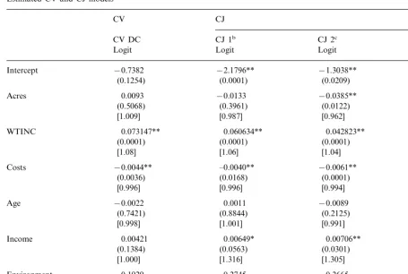
Estimated CV and CJ model coefficients are presented in Table 2. With the exception of acres, estimated CV coefficients were of the expected sign. However, only two variables, increase in wood turtle population and costs, were statisti-cally significant in all four models. The CJ model results were much more robust; all coefficients had the expected sign and relative to the CV model, more variables were statistically significant.
Estimated WTP was derived from the CV, CJ1, and CJ2 models for the ‘average’ EM program by using Eqs. (7) and (10). The estimated value of dV from Eq. (10) was substituted for dV in Eq. (7) and the probability of program acceptance was
5At-test was used to test for differences in socio-economic characteristics of CV and CJ respondents. The null hypothesis that the two groups are the same was not rejected for age, but was rejected for income. The mean income of CJ respondents ($59 844) was statistically different than the mean income of CV respondents ($55 151).
Table 2
Estimated CV and CJ modelsa
CV CJ
CJ 3d
CJ 1b CJ 2c
CV DC
Logit Logit Logit Tobit
−2.1796** 2.4867**
−0.7382
Intercept −1.3038**
(0.1254) (0.0001) (0.0209) (0.0437)
0.0093 −0.0133 −0.0385** −0.0797**
Acres
(0.3961)
(0.5068) (0.0122) (0.0180)
[0.987] [0.962]
[1.009]
0.042823** 0.060634**
WTINC 0.073147** 0.1133**
(0.0001) (0.0001) (0.0001) (0.0001)
[1.08] [1.06] [1.04]
−0.0154** –0.0040**
Costs −0.0044** −0.0061**
(0.0168) (0.0001) (0.001)
(0.0036)
[0.996] [0.996] [0.994]
0.0011 0.0104
−0.0022
Age −0.0089
(0.8844) (0.2125) (0.5044)
(0.7421)
[0.991]
[0.998] [1.001]
0.00421 0.00649* 0.00706**
Income 0.01362*
(0.1384) (0.0563) (0.0301) (0.0557)
[1.305] [1.316]
[1.000]
0.2745 0.2665 0.9791
Environment 0.1929
(0.1076) (0.3443)
(0.3300) (0.4547)
[1.213] [1.000] [1.000]
Observations 581 692 692 504
aThe values reported in the [ ] represent exp (b
j), the odds ratio statistic.
bDependent variable is 1 if individual would definitely undertake the program (i.e. rating=10); 0 otherwise. cDependent variable is 1 if individual rated program greater than the status-quo; 0 otherwise.
dDependent variable is rating difference from status-quo.
* The values reported in the ( ) arex2Pvalues significant at the 0.10 level. ** Significant at the 0.05 level.
obtained by multiplying the mean value of all independent variables, except cost, by the appro-priate estimated coefficients (Table 2). Median WTP was then derived by calculating the cost that yields a 0.5 payment probability (see Eq. (7)). Mean WTP values were calculated by integrating over the $0 to $200 cost range. The CJ3 WTP estimate was derived by finding the value for N which sets dV in Eq. (10) equal to zero.
Results of these calculations are presented in Table 3. As shown in Table 3, the CV and CJ 1
model WTP point estimates are very different.6It is important to emphasize that from the perspec-tive of economic theory and econometric tech-nique, these models are virtually identical. The only difference is that while CV respondents were asked if they would definitely pay a predetermined
Table 3
Estimated WTP values
CJ CV
CJ 1a CJ 2b
CV DC CJ3c
Logit Logit Logit Tobit
Estimated median $86 $−287 $211 $285 values
$86 $31 $116 –
Estimated mean valuesd
aDependent variable is 1 if rating is 10; 0 otherwise. bDependent variable is 1 if program rated above status-quo; 0 otherwise.
cDependent variable is ratings difference from status-quo. dMean values were calculated over the $0 to $200 cost range.
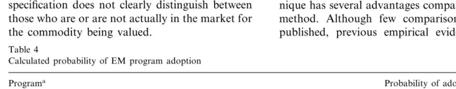
Estimated probabilities that respondents would undertake several different types of EM programs are presented in Table 4. These probabilities were derived by substituting the estimated value of dV from Eq. (10) into Eq. (7). As expected, probabil-ities based on the CJ1 model are much lower than those based on the CV or CJ2 model.
Despite sensitivity to model specification, it is important to note that the results reported in Table 4 suggest that many non-industrial forest landowners would be willing to undertake EM programs even though the benefits accrue down-stream and off the landowner’s property. For example, the probability that the average respon-dent would pay $100 per year for EM to increase the wood turtle population by 25% ranged from 0.32 to 0.78, depending on model specification (see Table 4).
Moreover, the probability of EM adoption ranged between 0.13 and 0.52 for a program which sets aside about a 12-acre buffer zone, results in :12% increase in the wood turtle population, and costs each landowner $200 per year. However, in interpreting these results it is important to remem-ber that since all survey respondents were already enrolled in a forest stewardship management pro-gram, the likelihood of EM program adoption is undoubtedly higher for this group than for the forest landowner population in general.
5. Conclusions
Many economists have argued that the CJ tech-nique has several advantages compared to the CV method. Although few comparisons have been published, previous empirical evidence suggests amount, CJ1 respondents were asked to rank each
EM option on a scale of 1 to 10 with 10 indicating that they would definitely undertake EM.
When comparing WTP estimates from the CJ2 and CJ3 model and the CV model, it is important to remember that CJ2 respondents are assumed to undertake all EM programs that were rated above the status quo, and the CJ3 specification assumes that rating difference is a cardinal measure of respondent preferences (Roe et al., 1996).
As expected, the CJ2 point estimate is greater than the CV estimate and this difference is statisti-cally different at the 95% level. The CJ2 WTP estimate is biased upward because it is implicitly assumed that all respondents who ‘might’ pay will, in fact, do so. The CJ3 model results should also be interpreted as an upper bound because this specification does not clearly distinguish between those who are or are not actually in the market for the commodity being valued.
Table 4
Calculated probability of EM program adoption
Probability of adoption Programa
CJ1
CV CJ2
0.18
0.48 0.66
$100 cost; 11.83 acre buffer zone; 11.85% increase in wood turtle population
0.38
$200 cost; 11.83 acre buffer zone; 11.85% increase in wood turtle population 0.13 0.52 0.32
0.71 0.78
$100 cost; 11.83 acre buffer zone; 25% increase in wood turtle population
0.32 0.06
0.22 $200 cost; 20 acre buffer zone; no increase in wood turtle population
that WTP estimates often differ dramatically. Sev-eral explanations for this have been offered. For example, Magat et al. (1988) argue that CV cre-ates incentives for respondents to understate their true WTP. On the other hand, Boxall et al. (1996) conclude that CV results may be biased upward because of ‘yea-saying’ and because respondents to the ‘typical’ CV survey consider fewer substitutes.
Our results suggest that when CV and CJ ques-tions are the same, except for rating and pricing format, WTP estimates are different. In particu-lar, since most previous CJ studies have essen-tially counted ‘maybe’ responses as ‘yes’ responses, we believe that CJ WTP estimates have often been biased upwards.
While no comprehensive conclusions can be drawn about landowner attitudes towards the ecosystem management approach, several points about EM can be drawn from this analysis. For example, many respondents would pay some amount for wood turtle habitat protection down-stream and off their own property. Also, for the three CJ models, the coefficient of landowner income was significantly positive, suggesting that landowner affluence and likelihood of participa-tion in EM are related.
This is only one case study and much more research about EM and comparing the CV and CJ techniques is needed. Although the CJ ap-proach seems to offer several conceptual advan-tages relative to CV, CJ is very sensitive to model specification. Although we agree with Boxall et al. (1996) that the CJ technique offers ‘considerable enhancements’ compared to CV and should there-fore by more widely used in the valuation of environmental programs, CJ results should cer-tainly be interpreted with caution.
Acknowledgements
This research was supported by funds provided by the US Department of Agriculture, Forest Service, Northeast Forest Experiment Station. We are indebted to two anonymous reviewers for helpful suggestions.
Appendix A. Conjoint survey
Please consider the situation shown below. Sup-pose that you own and reside on property number 2 which is adjacent to two other privately owned forested parcels. Each forested parcel contains about 50 acres. Two-hundred acres of state forest land is adjacent to one end of the forested parcels. Adjacent to the opposite end of the forest parcels is 600 acres of town wildlife conservation land. A stream runs through all five parcels of land. All land next to this stream is forested but is not suitable for any other land use, such as housing development. Wood turtles exist downstream on the town wildlife conservation land. It is impor-tant to view the five separate parcels as one regional ecosystem, where the environmental functions of each parcel are interconnected. That is, land management decisions on one parcel of land impact environmental functions on the sur-rounding parcels.
Suppose that you are asked to co-operate with your neighbors for the purpose of managing your land as part of a larger unit. Specifically, you are asked to agree to set aside, improve, and maintain a buffer zone on each side of the stream. Improve-ments include planting of shrubs along the stream bank to reduce damage from runoff and sediment to downstream areas. Final decisions about im-provements and the cost of all imim-provements will be shared equally with your neighbors. This buffer zone creates a natural wildlife corridor; it connects the two larger parcels of wildlife habitat, the state forest and town wildlife conservation land. The buffer zone also improves water quality downstream which is important for maintaining the wood turtle population located on the town wildlife conservation land.
A.1. Alternati6e A
Your rating You agree to set aside 10 acres
of your property for the buffer for
zone. Limited timber alternative A management, including harvest, is ….. (scale
1 to 10). could continue in this zone, but
please assume that this land is not suitable for other uses, such as housing development.
Population of the is wood turtle will increase by 0%.
Your share of improvement and maintenance costs associated with the buffer zone will be $50 per year This cost will also be incurred by your neighbors.
A.2. Alternati6e B
Your rating You agree to set aside 20 acres
for alternative of your property for the buffer
B is ….. zone. Limited timber
manage-(scale 1 to ment, including harvest, could
continue in this zone, but please 10). assume that this land is not suitable for other uses, such as housing development. Popula-tion of the wood turtle will in-crease by 10%. Your share of improvement and maintenance costs associated with the buffer zone will be $200 per year. This cost will also be incurred by your neighbors.
A.3. Alternati6e C
Your rating for Do nothing.
alternative C is ….. (scale 1 to 10). No buffer zone.
No increase in wood turtle population. You agree to set aside 5 acres
of your property for the buffer for alterna-tive D is ….. zone. Limited timber
manage-ment, including harvest, could (scale 1 to continue in this zone, but please 10). assume that this land is not
suitable for other uses, such as housing development. Popula-tion of the wood turtle will in-crease by 10%.
Your share of improvement and maintenance costs associated with the buffer zone will be $200 per year. This cost will also be incurred by your neigh-bors.
Appendix B. CV survey
Introduction and instructions to respondents; same as CJ survey (Appendix A).
Please consider and compare all the alternatives presented and then indicate which alternatives, if any, you would definitely undertake.
B.1. Alternati6e A
Would you You agree to set aside 10 acres
of your property for the buffer definitely un-dertake alter-zone. Limited timber
manage-native A? ment, including harvest, could
…..Yes continue in this zone, but please
…..No assume that this land is not
suitable for other uses, such as housing development. Popula-tion of the wood turtle will in-crease by 0%.
B.2. Alternati6e B
You agree to set aside 20 Would you acres of your property for definitely the buffer zone. Limited undertake
alternative B? timber management,
…..Yes including harvest, could
continue in this zone, but …..No please assume that this land
is not suitable for other uses, such as housing development. Population of the wood turtle will
increase by 10%.
Your share of improvement and maintenance costs associated with the buffer zone will be $200 per year. This cost will also be incurred by your neighbors.
B.3. Alternati6e C
Do nothing. Would you definitely undertake alternative C? …..Yes
…..No No buffer zone.
No increase in wood turtle population. No additional improvement or maintenance costs.
B.4. Alternati6e D
You agree to set aside 5 Would you acres of your property for definitely
undertake the buffer zone. Limited
timber management, alternative D? …..Yes including harvest, could
continue in this zone, but …..No please assume that this land
is not suitable for other uses, such as housing development. Population of the wood turtle will
increase by 10%.
Your share of improvement and maintenance costs associated with the buffer zone will be $200 per year. This cost will also be incurred by your neighbors.
References
Alberini, A., Boyle, K., Welsh, M., 1997. Using multiple-bounded questions to incorporate preference uncertainty in non-market valuation. In: Englin, J. (Compiler), Tenth Interim Report, W-133 Benefits and Costs Transfer in Natural Resource Planning, University of Reno, Reno, NV.
Barrett, C., Stevens, T.H., Willis, C., 1996. Comparison of CV and conjoint analysis in groundwater valuation. In: Her-riges, J. (Compiler), Ninth Interim Report, W-133 Benefits and Costs Transfer in Natural Resource Planning, Depart-ment of Economics, Iowa State University, Ames, IA. Bowker, J.M., Stoll, J.R., 1988. Use of dichotomous choice
nonmarket methods to value the whooping crane resource. Am. J. Agric. Econom. 70 (2), 372 – 381.
Boxall, P., Adamowicz, W., Swait, J., Williams, M., Laviere, J., 1996. A comparison of stated preference methods for environmental valuation. Ecol. Econom. 18, 243 – 253. Brown, T., 1984. The concept of value in resource allocation.
Land Econom. 60, 231 – 246.
Brunson, M.W., Yarrow, D., Roberts, S., Guynn, D., Kuhns, M., 1996. Nonindustrial private forest owners and ecosys-tem management. J. For. 94, 14 – 21.
Champ, P., Bishop, R., Brown, T., McCollum, D., 1997. Using donation mechanisms to value nonuse benefits from public goods. J. Environ. Econom. Manag. 32 (2), 151 – 162.
Desvouges, W.H., Smith, V.K., 1983. Option price estimates for water quality improvements: a contingent valuation study for the Monogahela river. J. Environ. Econ. Manag. 14, 248 – 267.
Elkstrand, E., Loomis, J., 1997. Estimated willingness to pay for protecting critical habitat for threatened and endan-gered fish with respondent uncertainty. In: Englin, J. (Compiler), Tenth Interim Report, W-133 Benefits and Costs Transfer in Natural Resource Planning, University of Reno, Reno, NV.
Gan, C., Luzar, E.J., 1993. A conjoint analysis of waterfowl hunting in Louisiana. J. Agric. Appl. Econom. 25, 36 – 45. Irwin, J.R., Slovic, P., Licktenstein, S., McClelland, G., 1993. Preference reversals and the measurement of environmen-tal values. J. Risk Uncertain. 6, 5 – 18.
Magat, W.A., Viscusi, W.K., Huber, J., 1988. Paired compari-son and contingent valuation approaches to morbidity risk valuation. J. Environ. Econom. Manag. 15, 395 – 411. McKenzie, J., 1993. A comparison of contingent preference
models. Am. J. Agric. Econom. 75, 593 – 603.
McKenzie, J., 1990. Conjoint analysis of deer hunting. North-eastern J. Agric. Resour. Econom. 19 (21), 109 – 117. Ready, R., Whitehead, J., Blomquist, G., 1995. Contingent
valuation when respondents are ambivalent. J. Environ.
Econom. Manag. 29 (2), 181 – 197.
Roe, B., Boyle, K., Teisl, M., 1996. Using conjoint analysis to derive estimates of compensating variation. J. Environ. Econ. Manag. 31, 145 – 159.
Stanley, T.R., 1995. Ecosystem management and the arro-gance of humanism. Conserv. Biol. 9 (2), 255 – 262. Wang, H., 1997. Treatment of don’t know? Responses in
contingent valuation survey: a random valuation model. J. Environ. Econom Manag. 32, 219 – 232.