Canalization as a non-genetic source of adaptiveness during
morphogenesis: experimental evidence from analysis of
reproductive development in
Sorghum bicolor
G. Nissim Amzallag
1Department of Plant Sciences,The Hebrew Uni6ersity of Jerusalem,Jerusalem91904,Israel Received 6 June 2000; accepted 8 June 2000
Abstract
In Sorghum bicolor, perturbations in reproductive development observed following salt-treatment also influence progeny grown in the absence of NaCl. However, a developmental reversion of these modifications may be observed throughout two successive generations. This response, termed canalization, does not spontaneously occur following growth in the absence of NaCl, but is triggered by the level of perturbation in parental expression of reproductive characters. Moreover, canalization is not specific to the perturbed character, but it includes modifications in reproductive development as a whole. A decrease in developmental variability coincides with amplitude of the developmental reversion. This phenomenon is interpreted as an evidence for orientation of the developmental process towards the lowest free-energy state of the ‘epigenetic landscape’. Involvement of this phenomenon of canalization in developmental stability, adaptiveness, and evolution is discussed. Moreover, these results point to the need for a posteriori methods of investigations in order to analyze self-organized transformations in biological systems. © 2000 Elsevier Science Ireland Ltd. All rights reserved.
Keywords:Adaptiveness; Canalization; Developmental plasticity; Evolvability; Non-genetic information; Self-organization www.elsevier.com/locate/biosystems
ally understood as the expression of a develop-mental homeostasis, a capacity of the developing organism to reach a final, defined state. It has been be related to a series of cybernetic regula-tions in metabolism and protein synthesis, directly or indirectly controlled by the pre-existing genetic information. However, this ‘teleonomic property’ of development seems more complex than as-sumed for at least three reasons.
The first is that, as emphasized by Waddington (1957, p. 121), ‘homozygotes seem usually to be
1. Introduction
The self-buffering capacity of development has been recognized for a long time. It was termed
equifinality (von Bertalanffy, 1950), correcti6e
pleiotropy (Warburton, 1955), or canalization
(Waddington, 1957). This phenomenon is
gener-1Present address: The Judea Center for Research and De-velopment, Carmel 90404, Israel. Fax: +972-2-9960061.
more variable in an inconstant environment than the heterozygotes are’, a situation incompatible with a complete genetic control of canalization. The second is that characters are generally nor-mally-distributed in wild populations in spite of a strong genetic and environmental variability (Bar-ton and Turelli, 1989). The third is that genetic information is not completely controlling develop-ment. There is rather a temporal alternance be-tween self-organized and direct genetic control, while self-organization is largely involved in the achievement of major developmental and physio-logical events (Sachs, 1994; Amzallag, 2000a,b).
Beyond these considerations, canalization strongly differs from developmental homeostasis in the capacity of development to tend towards the optimal end-result according to the internal or environmental constraint (Waddington, 1957, pp. 43 – 44). This adaptive aspect of canalization was clearly observed in plants (Bradshaw, 1965; Moran et al., 1981; Sultan, 1992) and was termed
adapti6e determinism by Seligmann and Amzallag
(1995).
Existence of a ‘developmental buffer’ seems very important for integration of complex physio-logical regulations, and evolution would require extremely rare combinations of simultaneous mu-tations in its absence (Warburton, 1955). In spite of the evidence, canalization was ‘unfairly under-played in evolutionary discussions’ (Alberch, 1980). It was also excluded from developmental and physiological considerations. This obscure sit-uation does not only result from a deterministic approach of development centered on expression of a pre-existing information, but we must also recognize that the phenomenon of canalization confounds investigation. The high velocity and efficiency of this process prevents any opportunity to identify transitory phases towards the ‘develop-mental resolution’. Fortunately, this process be-comes visible when it takes place over an extended period. For example, Oono (1985) described a dwarf mutation in some individuals regenerated from cultured cells of rice. Although this trait is due to an homozygous mutation, a ‘chimeric re-version’ towards normal stem height was observed in progeny of regenerated plants, and it remained stable for at least three successive generations.
This change was obviously directed, because a normal-to-dwarf transition has never been ob-served after plant regeneration (Oono, 1985). The requirement for two sexual generations suggests the occurrence of intermediate states in the devel-opmental reversion, which may be analyzed.
A similar opportunity exists inSorghum bicolor. In this species, a 3-week exposure to a moderate concentration of NaCl induces an ability to grow and set seeds at an otherwise lethal salinity. This response was defined assalt-adaptation(Amzallag et al., 1993). All the individuals of the salt-treated population were able to grow at the NaCl concen-tration lethal for non-treated plants, but induction of salt-adaptation was accompanied by a consid-erable increase in phenotypic diversity (Amzallag et al., 1995; Amzallag, 1999a). Salt-adapted plants displayed many perturbations in reproductive de-velopment (Amzallag, 1996, 1998), suggesting that canalization was disrupted by expression of salt-adaptation. The reproductive development was also disturbed in progeny of salt-adapted plants (Amzallag, 1996), even for individuals grown in absence of NaCl (Amzallag et al., 1998). More-over, the evidence for a ‘developmental reversion’ in reproductive development of progeny of salt-adapted plants was already suggested by previous observations (Amzallag and Seligmann, 1998). However, the latter analysis was complicated by re-exposure of the successive generations to a salt-adaptation treatment. The purpose of this study is to analyze the phenomenon of ‘develop-mental reversion’ in offspring of one or two suc-cessive generations of salt-adapted Sorghum that are grown in absence of NaCl.
2. Materials and methods
2.1. Plant material and growth conditions
2.1.1. Parental generations
Seeds from the MP610 genotype of S. bicolor
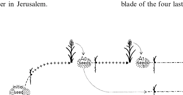
trans-ferred to 15 liter containers (12 seedlings per container, density of 80 plants m−2) filled with aerated half-strength Hoagland’s solution, accord-ing to Amzallag et al. (1993). Some plants, defined as control, were maintained in these conditions, were selfed and set seeds. Seeds from five control plants were harvested, and defined five lines of control progeny. On day 8 following imbibition, another subpopulation was exposed to 150 mM NaCl by six daily increases of 25 mM according to Amzallag (1998). These plants, defined as A0 plants, were maintained in this NaCl concentra-tion throughout their life cycle. They were selfed and set seeds. Seeds from six of these A0 plants defined six A0 lineages. A year later, seeds from these six lineages were germinated separately and treated for salt-adaptation as described for their A0 parents (Fig. 1). These A1 plants, also exposed to 150 mM NaCl until the end of their life cycle, were selfed and set seeds. For each A0 lineage, seeds of two A1 plants were harvested separately. All these plants were grown hydroponically throughout their life cycle. Media were changed weekly, and deionized water was added daily to the root medium in order to compensate for evapotranspiration. All the experiments were per-formed in a climatized greenhouse, under natural light intensity, and during the photoperiod of June – September in Jerusalem.
2.1.2. Field-grown progenies
Fifteen seeds from each one of the five control plants, the six A0 plants and the 12 corresponding A1 plants were soaked in a field at a density of four plants m−2. The 15 seeds from each line were separated in three groups of five seeds each, which were randomized in the different rows of the experiment. The plants were drip-irrigated with non-saline water (approx. 5 mM NaCl) throughout their life cycle. This experiment was performed for the three populations at the Gilat Experimental Station, from May to August of the same year. Field-grown progenies of the control, A0 and A1 plants are referred as the FC, FA0 and FA1 populations, respectively (Fig. 1). All the field-grown progenies issued from the same A0 ancestor (one FA0 line and two FA1 lines) defined a lineage. The six lineages have been separated into two classes of three lineages ac-cording to a criteria detailed in results below.
2.2. Measurements
The main stem of each plant was harvested after complete senescence of the shoot. After re-moving the seeds, the shoot was dried for two weeks at 60°C, weighed after removing all the blades, and defined as the shoot DW (SDW). The blade of the four last leaves was also weighed and
Table 1
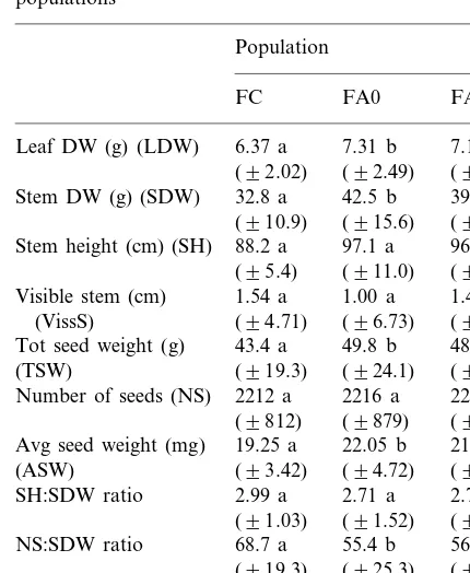
Comparison of mean (9SD) values of FC, FA0 and FA populationsa (910.9) (915.6) (913.9)
97.1 a
88.2 a 96.5 b
Stem height (cm) (SH)
(95.4) (911.0) (912.2)
Tot seed weight (g) 48.9 b
(TSW) (919.3) (924.1) (926.6) Number of seeds (NS) 2212 a 2216 a 2218 a
(9879)
(9812) (91068)
19.25 a 22.05 b
Avg seed weight (mg) 21.73 b
(93.42) (94.72) (95.54) (ASW)
SH:SDW ratio 2.99 a 2.71 a 2.75 a (91.52)
(91.03) (91.16)
55.4 b
NS:SDW ratio 68.7 a 56.2 b
(925.3)
(919.3) (926.4)
6.86 a
TSW:LDW ratio 6.78 a 6.74 a
(92.42)
(92.87) (93.24)
112
Population size 123 296
aA same letter following two values in the same row indicates that they are not distinguishable by a t-test at PB0.05.
SVL(C)=
2[C(L)-CFC] C(L)+CFC
where C(L) is the mean value of the character C for the line L, and CFCis the corresponding value calculated for the whole population of control plants (see Table 1). The absolute value of SVL(C) [abbreviated as ASVL(C)] quantifies the deviation of the line L from the FC population for expres-sion of the character C, and the sign (negative or positive) indicates direction of this discrepancy.
For each character C, the difference in ASV between FA1 and their corresponding FA0 line (abbreviated as DASVA1,A0(C) was calculated as follows: wherenis the number of lineages considered, and
mis the number of FA1 lines related to each FA0 line (n=3 and m=2 for classes I and II in the current experiment).
3. Results
3.1. The FC, FA0 and FA1 populations
Field-grown progeny of control and adapted plants (FC and FA0 plants respectively, see Fig. 1) were analyzed at the end of their life cycle. Stem height, weight and total seed weight signifi-cantly increased in FA0 plants, but the number of seeds and the length of the visible stem were not distinguishable from that of the FC plants (PB
0.05) by a t-test (Table 1). Relative to vegetative development, stem height and total seed weight (respectively SH:SDW and TSW:LDW ratios) of the FC and FA0 plants were similar, while a decrease in relative fertility (NS:SDW ratio) was observed in FA0 plants (Table 1). Progeny of two consecutive generations of salt-adapted plants (FA1 plants, see Fig. 1) was very similar (PB
0.05, t-tests) to the FA0 population for most of the characters analyzed (Table 1).
defined as the leaf DW (LDW). Stem height (SH) was defined as the length between the first adven-titious root and the top of the spike. The length of visible stem (VisS) was defined as the distance between the ligule of the last leaf and the first spikelet branch. This distance may be negative, as when the first spikelets developed below the ligule of the last leaf. The seeds were weighed and defined as the total seed weight (TSW). The aver-age seed weight (ASW) was determined after weighing three groups of ten seeds. The number of seeds was calculated as the ratio between total seed weight (TSW) and average seed weight (ASW).
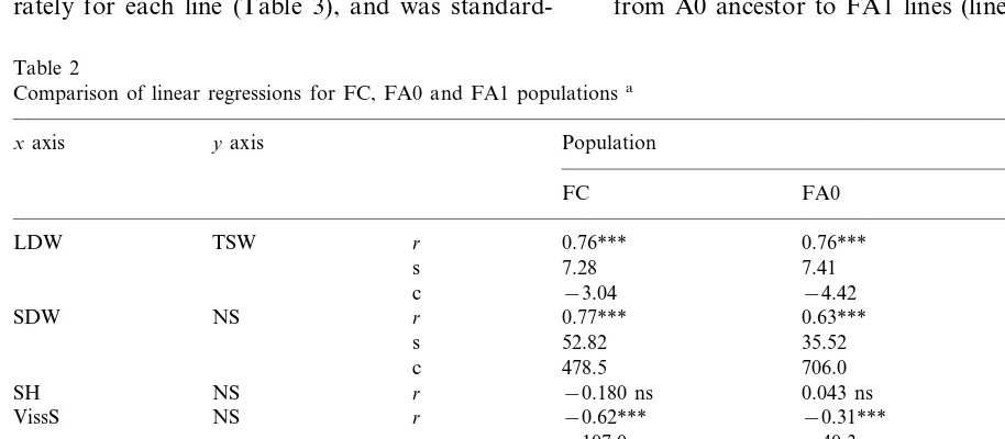
Correlations between characters were analyzed within each population. A highly significant rela-tionship was constantly observed between shoot DW and seed number (Table 2). Nevertheless, the slope of the linear regression differed for FA0 as compared with FC population, but also for FA1 as compared with FA0 (Table 2). This suggests that developmental regulations differed in the FA0 and FA1 populations. The FA1 plants issued from two successive treatments for salt-adaptation (Fig. 1). Enhancement of modifications was ex-pected for these plants, but this is not the case. The slope calculated for the FA1 population is generally intermediate between that of the FC and FA0 populations (Table 2), suggesting that the development reverted towards the ‘standard val-ues’ in the FA1 population.
3.2. E6idence for two classes of lineages
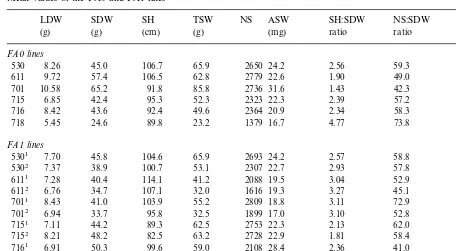
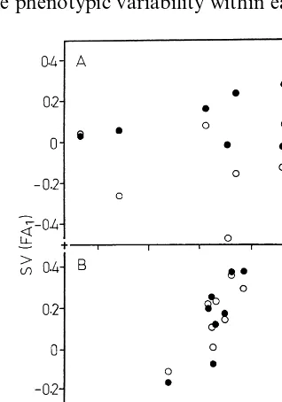
The FA0 and FA1 populations issued from the pooling of six FA0 and twelve FA1 lines respec-tively. All these 18 lines issued from six A0 ances-tors defining six lineages (see Section 2). The mean value of each character was calculated sepa-rately for each line (Table 3), and was
standard-ized (SV values) as described in Section 2. The length of visible stem was omitted from the results because of its considerable range of variations (Table 1). For each line, the SV indices calculated for the nine characters studied were pooled be-cause of the similar ranges of variation. Plotting the corresponding SV from two lines provides an estimate of their level of similarity. No significant correlation has been observed between the FA0 line and any one of the FA1 lines of the lineage 701 (Fig. 2A). In contrast, a significant positive correlation (PB0.05) was observed between FA0 and FA1 lines of the lineage 715 (Fig. 2B). A similar analysis was performed for the four other lineages. A significant correlation (PB0.05) may be seen between FA0 and FA1 lines in lineages: 530, 715 and 716, and the standardized values of the two corresponding FA1 lines also showed significant correlations (Table 4). The FA1 lines do not resemble the corresponding FA0 line in the lineages 611, 701 and 718, although the two sponding FA1 lines may show a significant corre-lation (lineage 611, Table 4). This analysis reveals that, in spite of initial homogeneity, all the lin-eages are not identical. The high ‘transmissibility’ from A0 ancestor to FA1 lines (lineages 530, 715
Table 2
Comparison of linear regressions for FC, FA0 and FA1 populationsa
xaxis yaxis Population
FC FA0 FA1
LDW TSW r 0.76*** 0.76*** 0.65***
s 7.28 7.41 7.28
−3.04
c −4.42 −3.12
SDW NS r 0.77*** 0.63*** 0.60***
35.52 45.96
s 52.82
386.1 706.0
478.5 c
r −0.180 ns 0.043 ns −0.055 ns
SH NS
VissS NS r −0.62*** −0.31*** −0.46***
−40.3
−107.0 −76.9
s
2257 2333
c 2377
SH r
VissS 0.58*** 0.59*** 0.46***
s 0.67 0.97 0.88
c 87.2 96.1 95.2
SDW SH r −0.003 ns 0.006 ns −0.031 ns
d.f. 110 121 294
Table 3
Mean values of the FA0 and FA1 linesa
LDW SDW SH TSW NS ASW SH:SDW NS:SDW TSW:LDW
(mg)
(g) (g) (cm) (g) ratio ratio ratio
FA0lines
45.0
530 8.26 106.7 65.9 2650 24.2 2.56 59.3 7.94
9.72 57.4 106.5 62.8 2779
611 22.6 1.90 49.0 6.45
701 10.58 65.2 91.8 85.8 2736 31.6 1.43 42.3 8.09
6.85 42.4 95.3
715 52.3 2323 22.3 2.39 57.2 7.54
8.42 43.6 92.4 49.6 2364
716 20.9 2.34 58.3 5.88
5.45 24.6 89.8 23.2 1379
718 16.7 4.77 73.8 4.32
FA1lines
45.8 104.6 65.9
5301 7.70 2693 24.2 2.57 58.8 8.56
5302 7.37 38.9 100.7 53.1 2307 22.7 2.93 57.8 6.78
7.28 40.4 114.1 41.2 2088
6111 19.5 3.04 52.9 5.68
6.76 34.7 107.1 32.0 1616
6112 19.3 3.27 45.1 4.35
8.43 41.0 103.9 55.2 2809
7011 18.8 3.11 72.9 6.78
7012 6.94 33.7 95.8 32.5 1899 17.0 3.10 52.8 4.24
7151 7.11 44.2 89.3 62.5 2753 22.3 2.13 62.0 8.70
7152 8.21 48.2 82.5 63.2 2728 22.9 1.81 58.4 7.74
6.91 50.3 99.6 59.0 2108
7161 28.4 2.36 41.0 8.38
9.77 61.3 94.0 75.2 2584
7162 29.6 1.64 45.0 8.05
7.62 54.2 98.1 71.8 2642
7181 28.1 2.15 48.2 9.19
7182 5.75 35.9 98.5 1.3 2015 20.1 3.32 57.1 7.23
aSame abbreviations as in Table 1.
cant correlation has been observed between mean ASV values of FA0 and FA1 populations belong-ing to Class I but not to Class II (Fig. 3A). This result confirms that the deviation from standard-ized value in development is similar for FA0 and FA1 populations in Class I. In Class II, however, the ASV were considerably reduced in FA1 as compared to FA0 populations (Fig. 3A).
The difference between ASV of the FA0 and the corresponding FA1 lines was estimated sepa-rately for Class I and Class II lineages. For each character C, the difference in ASV between FA1 and their corresponding FA0 line (abbreviated as DASVA1,A0(C), see Section 2) was calculated and plotted as a function of the mean ASV calculated for the corresponding FA0 lines (Table 5). No relationship was found in Class I lineages, but most of the DASV indexes were positive. This indicates that development was even more per-turbed in FA1 than in FA0 plants in Class I (Fig. 3B). A significant negative correlation (PB0.05) is observed in Class II lineages (Fig. 3B). This and 716) defined a Class I of lineages, while the
low ‘transmissibility’ (lineages 611, 701 and 718) defined a Class II of lineages.
3.3. Re6ersion towards normal de6elopment in
FA1 lines
Deviation from the standardized values was analyzed separately for the two classes of lineages. For each character, the absolute value of SV (termed ASV, see Section 2) was averaged for the three FA0 lines belonging the same class. Except for stem height, the ASV is always higher for FA0 from Class II than those from Class I (Table 5). This indicates that the FA0 plants belonging to Class II were the most modified in their development.
signifi-suggests that the tendency to recover the standard value in FA1 lines (negative DASV indexes) was proportional to the deviation observed in the FA0 line belonging to Class II.
3.4. Influence on6ariability
The phenotypic variability within each FA1 line
Table 5
Discrepancy from standard values in FA0 lines from Clases I and II. The absolute standard value (ASV) calculated for the three FA0 lines in the same class were averaged for each character The ASV calculated for each class are averaged as a mean ASV valuea
Character Absolute standard value (ASV) Class I Class II
0.203 0.355
Leaf DW
Stem DW 0.284 0.497
Stem height 0.104 0.080
0.244 0.542
Tot seed weight
0.262 0.152
Avg seed weight
SH:SDW ratio 0.206 0.537
0.294 NS:SDW ratio 0.164
0.226 TSW:LDW ratio 0.131
0.176
Mean ASV value 0.343
aAbbreviations as in Table 1.
Fig. 2. Relationship between FA0 and FA1 lines from the same lineage. (A) Lineage 701; (B) lineage 715. The standard values (SV indexes) were calculated from data of Tables 1 and 3 as described in Section 2. Solid circles: FA11 line; opened circles: FA12line.
Fig. 3. Relationship between perturbation in FA0 and FA1 plants. (A) Comparison of standardized values (ASV). (B) Influence of the perturbation in FA0 on the corrective effect (DASV) in FA1. Absolute standardized values (ASV) and their difference between FA0 and FA1 lines (DASV) are calculated from data in Table 5 as detailed in Section 2. Open circles: class I lineages; solid circles: class II lineages. Table 4
Comparison of two lines from the same lineagea rcoefficient between
Lineage
FA0 and
FA0 and FA11and
FA12 FA11 FA12
0.981* 0.887* 0.883* 530
0.583
611 0.246 0.902*
0.496
701 −0.014 0.408
0.959* 0.901*
0.902* 715
716 0.655 0.868* 0.884*
−0.801* 0.233 0.232 718
was analyzed separately for the two classes. For each one of the FA1 line, the coefficient of variation (abbreviated as CV) was calculated for each one of the nine characters. Variability within FA1 lines is generally greater that variability of the FC popula-tion (Table 6). Moreover, significant differences may be observed in the level of variability between the two classes. Variability is considerably in-creased in FA1 lines of Class II for the number of seeds or the relative stem height, but the situation is reversed for average seed weight (Table 6). Accordingly, lineages belonging to Classes I and II cannot be simply distinguished by this analysis. The CV values of the two FA1 lines from the same lineage were plotted together. No relationship is observed in Class I (P\0.05, Fig. 4A), while a significant positive correlation (r=0.50, 25 d.f.,
PB0.01) appears in Class II (Fig. 4B).
A capacity for developmental reversion was especially observed in Class II lineages (Fig. 3), which also showed a ‘control’ of variability (Fig. 4B). The link between these two types of events was tested. For each FA1 line and for each character, the coefficient of variation was standardized as a
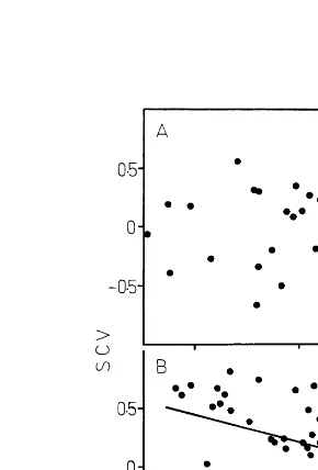
function of the average CV value of the character calculated for the FC population (see Table 5). These standardized values (abbreviated as SCV) were calculated as described above for mean values (SV, see Section 2). Then, for each character and for each FA1 line, the standardized coefficient of variation (SCV) was plotted as a function of the standardized mean value (SV). No significant rela-tionship (P\0.05) appears for FA1 lines of Class I (Fig. 5(A)), while a negative significant correlation (PB0.01) is observed for FA1 lines of Class II (Fig. 5(B)).
4. Discussion
4.1. Methodological considerations
An a posteriori distinction between two classes of lineages is problematic, because the same crite-rion cannot separate populations and be used to derive conclusions regarding their differences. Without any independent criterion of separation of the classes, the discrepancy from standard values observed in FA0 but not in FA1 of Class II may
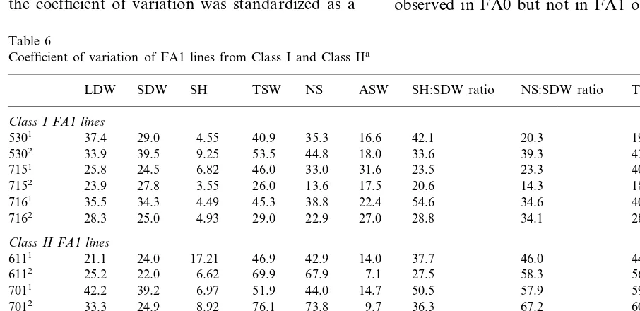
Table 6
Coefficient of variation of FA1 lines from Class I and Class IIa
LDW SDW SH TSW NS ASW SH:SDW ratio NS:SDW ratio TSW:LDW ratio Class I FA1lines
37.4 29.0 4.55 40.9
5301 35.3 16.6 42.1 20.3 19.3
25.0 4.93 29.0 22.9 27.0 28.8 34.1 28.2
28.3 7162
Class II FA1lines
46.0
51.9 44.0 14.7 50.5 57.9
7011 42.2 39.2 6.97 59.5
33.3 24.9 8.92 76.1
7012 73.8 9.7 36.3 67.2 60.5
19.9 33.7 6.76 34.6
7181 39.5 18.9 51.9 29.2 28.2
35.3 35.0 4.33 47.2
7182 41.8 17.3 52.7 22.0 39.5
Fig. 4. Relationship between variability within two FA1 lines from the same lineage. (A) Class I lines, (B) Class II lines. For each parameter, the standardized values of coefficient of varia-tion (SCV, see Secvaria-tion 3) of a FA1 line is plotted as a funcvaria-tion of the corresponding value for the other FA1 lines from the same lineage. No significant correlation is observed in 4(A) (r=0.0098, 25 d.f.), while a positive significant correlation (PB0.01) appears in 4(B) (r=0.50, 25 d.f.).
parameters is not verified, because salt-adaptation generates plurimodal distributions (Amzallag, 1998); (ii) A third source of variability has been identified during the process of salt-adaptation. This source is neither genetic nor environmental (Amzallag, 1999a), but is generated by self-orga-nized processes involved in critical phases in de-velopment (Amzallag, 2000a,b). Accordingly, analysis of the variability cannot be analyzed by ANOVA, nor can it be analyzed by any other method requiring a definition of the groups before the experiment. A posteriori segregation of the initially homogeneous population remains the only way to analyze the phenomenon of ‘develop-mental reversion’. Moreover, it is likely that phe-nomena of developmental reversion are so frequently ignored because of the methodological limitations of analyses based on an a priori segregation.
Fig. 5. Relationship between deviation in mean and CV values in FA1 lines. (A) Class I lines, (B) Class II lines. For each parameter and for each FA1 line, the standardized mean value (SV) is plotted as a function of the standardized CV value (SCV, see Section 3). No significant correlation (P\0.05) is observed in 5(A) (r=0.031, 52 d.f.), while a negative signifi-cant (PB0.01) correlation is observed in 5(B) (r= −0.357, 52 d.f.).
be explained as a random fluctuation in some FA0 plants, eventually due to an artifactual mod-ification of the environment. However, the ‘ran-dom fluctuation hypothesis’ cannot explain both the differences in variability between the two classes (Fig. 4) and the link between perturbation and variability (Fig. 5). The range of expression and variability of the characters is similar for the two classes, but the link is observed only in Class II. Consequently, analysis of variability provides the validation for methodological segregation be-tween the two classes of lineages in the initially homogeneous population.
4.2. The phenomenon of canalization
Offspring of salt-adapted plants are modified in their reproductive development (Table 1). How-ever, even in the absence of selection (see Section 2), modifications are reduced after two genera-tions of salt-adaptation treatment (Table 2). The fact that FA1 plants developed in a non-salinized medium is not sufficient to explain this phe-nomenon because deviation occurred specifically in some of the FA1 lines (Class II lineages, Table 4). Moreover, deviation is larger for FA0 than for FA1 plants (Table 2) although they were grown in the same environment at the same time (see Sec-tion 2). These consideraSec-tions confirm that salt-adaptation induces modifications in reproductive development (Amzallag, 1998), which are able to influence the next generation (Amzallag, 1996; Amzallag et al., 1998). They reveal a capacity to recover an almost-normal development after more than one generation of salt-adaptation.
A similar recovery of perturbations has been observed in plants regenerated from cultured cells following two sexual generations (Oono, 1985; Morrish et al., 1990; Cheng et al., 1992). In general, such a phenomenon has been interpreted as a reversion, assuming that the modifications were caused by reversible genetic changes (such as changes in the pattern of cytosine methylation) leaving the DNA sequence unaffected. Accord-ingly, the phenomenon of reversion is interpreted as an elimination of the stress-induced modifica-tion following re-exposure to the optimal condi-tions. Such an interpretation cannot be rejected, but is not likely in the present case, because developmental reversion also occur for plants maintained in salinity for many generations (Amzallag and Seligmann, 1998). Moreover, a capacity to recover an almost-initial status was clearly demonstrated after occurrence of non-re-versible genetic changes.
Working with maize mutants, Martienssen et al. (1990) described a non-random modification in the genome structure, during the early vegetative development, which enabled the seedlings to re-cover a wild-type phenotype. They suggested that a genetic mechanism is able to restore a functional morphogenetic capacity, in spite of non-reversible
modifications accumulated during previous gener-ations. Such a phenomenon also occur during normal development. For example, the cellular DNA content of embryos of Dasypirum 6illosum
(Graminae) varies relatively to position of the caryopse on the spike (Frediani et al., 1994). This variation is not due to a change in polyploidy, but rather to amplification and/or deletion of specific repetitive DNA sequences. Nevertheless, the DNA content is buffered towards a ‘standard value’ during the early development of the progeny of low or high DNA content. This pro-cess is not random: repetitive DNA sequences which were the most deleted are preferentially amplified during this self-regulation process (Fre-diani et al., 1994). These examples indicate that a property of auto-regulation exists at the genome level despite large non-reversible modifications (see Amzallag, 1999b and references therein). Canalization, as defined by Waddington (1957), does not imply any reversibility of the changes involved in expression of the characters temporar-ily modified. For this reason, canalizationis more appropriate than re6ersion to describe this
phenomenon.
4.3. Mechanisms of canalization
The developmental perturbation was not al-ways higher in Class II plants than in Class I ones (Table 5). However, at a similar level of deviation, Class II plants showed canalization while Class I plants did not (Fig. 3). This suggests that canal-ization is not expressed independently for each parameter, but is triggered for the reproductive development as a whole, in response to a global level of perturbation.
explains why canalization may be observed for the reproductive development as a whole, and not only for the characters with the most perturbation (Fig. 3).
The recovery of reproductive development through isolation from the vegetative organs is expected only in the case of informational redun-dancy between, and within, successive phases of development. Such redundancy of the information was recognized as a factor in the stability of development (Conrad, 1990; Chauvet, 1993), and it was experimentally observed during vegetative development in S. bicolor (Amzallag, 1999c). Thus, it is likely that canalization in reproductive development is reached by elimination of the dis-turbing element (the linkage with the previous phase of development modified by salt-adapta-tion) of this redundant informative system.
A negative correlation between level of variabil-ity and mean value (respectively, SCV and SV) was observed only for FA1 lines of Class II (Fig. 5). This indicates that low variability is not di-rectly related to expression of the standard values (Fig. 5(A)), but that it is especially reduced by the process of canalization itself (Fig. 5(B)). In other words, the decrease in variability is linked to recovery of an optimal value. This suggests that optimal values act as ‘thermodynamic basins of attraction’ (see Conrad (1990) for discussion of this notion) for the process of canalization. Ac-cordingly, canalization becomes an expression of the spontaneous tendency of (living) open systems to reach their minimum free-energy level (Pri-gogine and Wiame, 1946; von Bertalanffy, 1950).
5. Conclusions
The above considerations confirm that (i) varia-tions in biological systems are not continuous, but discrete, at many (if not all) scales of organiza-tion; (ii) an initial (or almost-initial) state may be restored in spite of nonreversible transformations (see Section 1); (iii) biological processes tend to-wards optimal and/or adaptive status (Conrad, 1983). This latter process involves emergence of a network of interactions between tissues develop-ing concomitantly (Amzallag, 2000a), as well as an adaptive reorganization of the whole organism
towards the newly-emerging structures (Amzallag, 1999d).
These conclusions illustrate how the property of canalization and its adaptive dimension may be described by simple thermodynamic models, with-out any necessity for specific genes to correct the development and to govern morphogenesis to-wards defined values. Simultaneously, it intro-duces a serious entanglement with the classical representation of phenotype-genotype relation-ships. It suggests that a phenotype results from genome/environment interactions towards discrete final states of high stability, which are controlled by the process of development itself (Amzallag, 2000a). As Alberch (1980) claimed, ‘In evolution, selection may decide the winner of a given game but development non-randomly defines the players’.
In spite of its importance, this self-developmen-tal factor may be easily ignored under optimal conditions, because redundancy in processes con-trolling development lead to monomodal distribu-tions of characters. Under these condidistribu-tions, the illusion of a development strictly controlled by genetic information is even intensified by predicti-bility generated by high stapredicti-bility of the basins of attraction. However, this ‘developmental land-scape’ may be strongly modified under specific exposure to unfavorable environment. Heslop-Harrison (1959) and Amzallag (1999a) noticed that the sudden and extensive increase in variabil-ity observed in modified environments cannot be related to a genetic and/or environmental hetero-geneity. A third, self-developmental, factor is able to canalize development towards adaptive states. In optimal conditions, this adaptive response ori-entates development towards ‘recovery’ of stan-dard values.
exists on all levels, from genome to entire organism.
From a thermodynamic point of view, a devel-oping organism oscillates between an extensively-opened system (during transitory periods) and a minimally-opened system (during phenophases) (Amzallag, 2000b). The latter becomes stabilized by a network of homeostatic regulations set dur-ing transitory periods. However, the self-orga-nized nature characterizing transition periods generates both variability through extreme sensi-tivity to the initial conditions (Amzallag, 1999a), and adaptability through evolution towards the lowest free-energy level (Conrad, 1983). Accord-ingly, within a specific range of variation of the initial conditions, adaptive properties of the tran-sition period generate a unifying developmental process, a canalization. However, it is the same process which also generates adaptive modifica-tions of the phenotype, beyond a critical level of variation in inital conditions.
Including such an adaptive dimension in mor-phogenesis modifies our definition of a species. A species, characterized by specific morphological traits, becomes the expression of a stable ‘‘devel-opmental landscape’’ generating a definite mor-phological pattern within a specific range of genetic and environmental diversity.
Acknowledgements
I would thank to Professor Avi Nachmias, from the Gilat Experimental Station for his help in performing the field experiment; Liviu Liviescu for technical and agronomical assistance, and to Nili Avni, Liat Gonen and Benyamin Zeit for harvesting and parameter measurements.
References
Alberch, P., 1980. Ontogenesis and morphological diversifica-tion. Am. Zool. 20, 653 – 667.
Amzallag, G.N., 1996. Influence of parental NaCl treatment on salinity tolerance of offspring in Sorghum bicolor(L.) Moench. New Phytol. 128, 715 – 723.
Amzallag, G.N., 1998. Induced modifications in reproductive traits of salt-treated plants ofSorghum bicolor. Isr. J. Plant Sci. 46, 1 – 8.
Amzallag, G.N., 1999a. Individuation in Sorghum bicolor: a self-organized process involved in physiological adaptation to salinity. Plant Cell Env. 22, 1389 – 1399.
Amzallag, G.N., 1999b. Plant evolution: towards an adaptive theory. In: Lerner, H.R. (Ed.), Plant Responses to Envi-ronmental Stresses: from Phytohormones to Genome Re-organization. Dekker, New York, pp. 171 – 245.
Amzallag, G.N., 1999c. Regulation of growth: the meristem network approach. Plant Cell Env. 22, 483 – 493. Amzallag, G.N., 1999d. Adaptive nature of the transition
phases in development: the case ofSorghum bicolor. Plant Cell Env. 22, 1035 – 1041.
Amzallag, G.N., 2000a. Connectance in Sorghum develop-ment: beyond the genotype-phenotype duality. BioSystems 56, 1 – 11.
Amzallag G.N., 2000b. The adaptive potential of plant devel-opment: evidence from the response to salinity. In: La¨uchli A., Lu¨ttge U. (Eds.), Salinity: Environment — Plants — Molecules. Kluwer, The Netherlands. In press.
Amzallag, G.N., Seligmann, H., 1998. Perturbation in leaves of salt-treatedSorghum: elements for interpretation of the normal development as an adaptive response. Plant Cell Env. 21, 785 – 793.
Amzallag, G.N., Seligmann, H., Lerner, H.R., 1993. A devel-opmental window for salt-adaptation inSorghum bicolor. J. Exp. Bot. 44, 645 – 652.
Amzallag, G.N., Seligmann, H., Lerner, H.R., 1995. Induced variability during the process of adaptation in Sorghum bicolor. J. Exp. Bot. 45, 1017 – 1024.
Amzallag, G.N., Nachmias, A., Lerner, H.R., 1998. Influence of the mode of salinization on the reproductive traits of the field-grown progeny inSorghum bicolor. Isr. J. Plant Sci. 46, 9 – 16.
Barton, N.H., Turelli, M., 1989. Evolutionary quantitative genetics: how little do we know? Ann. Rev. Genet. 23, 337 – 370.
Bertalanffy von, L., 1950. The theory of open systems in physics and biology. Science 111, 23 – 29.
Bradshaw, A.D., 1965. Evolutionary significance of pheno-typic plasticity in plants. Adv. Genet. 13, 115 – 155. Chauvet, G.A., 1993. Hierarchical functional organization of
formal biological systems: a dynamical approach. I. The increase in complexity by self-association increases the domain of stability of a biological system. Phil. Trans. R. Soc. Lond. B 339, 425 – 444.
Cheng, X.Y., Gao, M.W., Liang, Z.Q., Liu, G.Z., Hu, T.C., 1992. Somaclonal variation in winter wheat: frequency occurance and inheritance. Euphytica 64, 1 – 10.
Conrad, M., 1983. Adaptability — The Significance of Vari-ability from Molecule to Ecosystem. Plenum, New York. Conrad, M., 1990. The geometry of evolution. BioSystems 24,
61 – 81.
Heslop-Harrison, J., 1959. Variability and environment. Evo-lution 13, 145 – 147.
Lewontin, R.C., 1974. The analysis of variance and the analy-sis of causes. Am. J. Hum. Genet. 26, 400 – 411.
Martienssen, R., Barkan, A., Taylor, W.C., Freeling, M., 1990. Somatically heritable switches in the DNA modifica-tion of Mutransposable elements monitored with a sup-pressible mutant in maize. Genes Develop. 4, 331 – 343. Moran, G.F., Marshall, D.R., Muller, W.J., 1981. Phenotypic
variation and plasticity in the colonizing speciesXanthium strumarium. Austr. J. Biol. Sci. 34, 639 – 648.
Morrish, E.M., Hanna, W.W., Vasil, I.K., 1990. The expres-sion and perpetuation of inherent somatic variation in regenerants from embryogenic cultures ofPennisetum glau -cum(pearl millet). Theor. Appl. Genet. 80, 409 – 416.
Oono, K., 1985. Putative homozygous mutations in regener-ated plants of rice. Theor. Appl. Genet. 198, 377 – 384. Prigogine, I., Wiame, J.M., 1946. Biologie et
thermody-namique des phe´nome`nes irre´versibles. Experentia 2, 451 – 453.
Sachs, T., 1994. Variable development as a basis for robust pattern formation. J. Theor. Biol. 170, 423 – 425. Seligmann, H., Amzallag, G.N., 1995. Adaptive determinism
during salt-adaptation inSorghum bicolor. BioSystems 36, 71 – 77.
Sultan, S.E., 1992. Phenotypic plasticity and the neo-dar-winian legacy. Evol. Trends Plants 6, 61 – 71.
Waddington, C.H., 1957. The Strategy of Genes. Allen and Unwin, London.
Warburton, F.E., 1955. Feedback in development and its evolutionary significance. Am. Natur. 89, 129 – 140.