Identi
"
cation of aggregate resource and job set characteristics
for predicting job set makespan in batch process industries
Wenny H.M. Raaymakers, Jan C. Fransoo*
Department of Operations Planning and Control, Eindhoven University of Technology, P.O. Box 513, Pav. F12, 5600 MB Eindhoven, Netherlands
Received 27 March 1998; accepted 6 September 1999
Abstract
We study multipurpose batch process industries with no-wait restrictions, overlapping processing steps, and parallel resources. To achieve high utilization and reliable lead times, the master planner needs to be able to accurately and quickly estimate the makespan of a job set. Because constructing a schedule is time consuming, and production plans may change frequently, estimates must be based on aggregate characteristics of the job set. To estimate the makespan of a complex set of jobs, we introduce the concept of job interaction. Using statistical analysis, we show that a limited number of characteristics of the job set and the available resources can explain most of the variability in the job interaction. ( 2000 Elsevier Science B.V. All rights reserved.
Keywords: Batch process industries; Multipurpose; Regression analysis; Order release; Scheduling
1. Introduction
Batch (chemical) processes exist in many indus-tries, such as the food, specialty chemicals and pharmaceutical industry, where production vol-umes of individual products do not allow continu-ous or semi-continucontinu-ous processes. Batch processing becomes more important because of the increasing product variety and decreasing demand volumes for individual products. Two basic types are distin-guished. If products all follow the same routing, this
is called multiproduct. If products follow di!erent
routings, like in a discrete manufacturing job shop,
*Corresponding author. Tel.:#31-40-2472681; fax: #31-40-2464596.
E-mail address:[email protected] (J.C. Fransoo).
it is calledmultipurpose. In this paper, we
concen-trate on multipurpose batch process industries. Multipurpose batch process industries produce
a large variety of di!erent products that follow
di!erent routings through the plant. Considerable
di!erences may exist between products in the
num-ber and duration of the processing steps that are required. Intermediate products may be unstable, which means that a product needs to be processed further without delay. These no-wait restrictions
and the large variety of products with di!erent
routings cause complex scheduling problems.
Namely, for each product a di!erent combination
of resources is required in a speci"c sequence and timing due to these no-wait restrictions. Conse-quently, the capacity utilization realized by multi-purpose batch process industries is generally low. Furthermore, many of these companies operate in
highly variable and dynamic markets in which peri-ods of high demand may be followed by periperi-ods of low demand. Therefore, the amount and mix of
production orders may di!er considerably from
period to period. Consequently, bottlenecks may shift over time due to variations in the mix of production orders.
One of the primary di$culties for this type of
industries is to estimate the workload that can be
completed during a speci"c period. Namely, the
capacity utilization that can be realized in a plan-ning period strongly depends on the current mix of production orders [1]. It is important for planners to accurately estimate what workload and mix of production orders can be completed in a period, in order to set reliable due dates to customers.
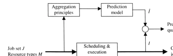
We assume a situation with hierarchical produc-tion control in which the (master) planner is
re-sponsible for selecting achievable sets of
production orders (jobs) per planning period. Hier-archical structures like this are very common in industry and have been described in many (text) books (e.g., [2,3]). A production plan for a period is considered achievable if a schedule can be construc-ted that completes all production orders before the end of that period. For the"rst period only, the job set is released to a scheduler that constructs a de-tailed schedule. This schedule is then executed at a production department. The planning horizon of the scheduler is much shorter than the planning horizon of the (master) planner. The (master) plan-ner may evaluate the achievability of the job sets for subsequent planning periods by constructing a schedule for each planning period. This would result in constructing a detailed schedule over a me-dium term horizon. The main disadvantage of this approach is that it is very time consuming, since a new schedule has to be constructed every time when a change in the plan occurs. Therefore, we prefer methods that assess the achievability of job sets based on aggregate information.
In this paper, we investigate characteristics of the job mix and of the resources in a production de-partment, to identify the characteristics that signi"
-cantly in#uence the completion time (makespan) of
a fully speci"ed job set. These characteristics may then be used to predict the makespan of a job set. In that way, a job set is expected to be achievable if the
predicted makespan is shorter than the length of a planning period. This provides an aggregate method to assess the achievability of job sets. The main advantage of this approach is that it provides the opportunity to make customer order accept-ance decisions quickly because computational e!ort is small.
This paper is organized as follows. The following section discusses the relevant literature. Section 3 gives the basic assumptions underlying the model. Section 4 describes the factors that we expect to be of in#uence on the job interaction. Then, the experi-mental design is described that is used to investi-gate if the interaction factors have a relation with the idle time required in the schedule or not. Sec-tion 6 includes the experimental results and statist-ical analysis. The last section contains the conclusions and suggestions for further research.
2. Literature
Makespan prediction is related to#ow time
pre-diction, which has received considerable attention in the literature. For an overview, we refer to the paper by Cheng and Gupta [4]. Flow time is the total throughput time of a job in a production system, which consists of processing time and wait-ing time. Flow time prediction is generally used in the determination of achievable due dates for cus-tomer orders. Upon arrival of a cuscus-tomer order, the
#ow time is estimated for the job related to that
customer order. The due date of the job is set to the
arrival date plus a #ow allowance, which is the
estimated#ow time. Several rules for determining
#ow time allowances are proposed in the literature.
A distinction can be made between rules that use job characteristics only, and rules that also use shop information. A simple and popular rule that uses job characteristics only, is the total work-rule.
According to this rule, the#ow time allowance is
proportional to the total processing time of the job
[5}8]. Bertrand [9] introduced a rule that uses
both the total processing time of a job and the
number of processing steps to determine the#ow
waiting time per job or per processing step as
a basis for #ow time prediction [5,6]. Also, the
number of jobs in the queues can be used for#ow
time prediction. Some of these rules use informa-tion on the total workload or total number of jobs in the shop, while others use only information of
the resources on the job's routing. Bertrand [9]
introduced the use of time-phased workload to
estimate the #ow time of a job. Vig and Dooley
[10] introduced the use of the average#ow time per
processing step of three recently completed jobs to
estimate the#ow time of a new job. The di!erent
job characteristics and shop congestion character-istics may also be used in combination to determine
the#ow time allowance. Some authors [10}12] use
regression analysis to determine the weighing
coef-"cients for the di!erent job and shop characteristics
included in the #ow time predictions. The
charac-teristics included, and the corresponding coe$
-cients, depend on the dispatching rule that is used for the execution of the jobs on the resources in the shop. Vig and Dooley [12] showed that using
com-bined static and dynamic #ow time prediction
methods yield#ow time predictions that are more
accurate and more robust to variable shop
condi-tion, than realized by dynamic#ow time prediction
methods.
A comparison of di!erent rules shows that using
information on the shop status improves the #ow
time prediction [5,6]. Furthermore, using informa-tion on the number of jobs or the workload in the
queues along the job's routing performs better than
using general shop congestion information [10,11]. From the literature, we conclude that both job information, such as the number of processing
steps, and shop congestion information in#uence
the #ow time. Therefore, we investigate whether
these characteristics also in#uence the makespan of
a job set in multipurpose batch process industries.
However, two important di!erences exist between
the situation considered in the literature and the situation considered in this paper. First, in the literature, traditional job shops are considered, whereas in this paper, we consider multipurpose
batch process industries. These di!er from
tradi-tional job shops in the no-wait restrictions between processing steps and the possible overlap of pro-cessing steps. Second, in the literature,#ow times of
individual jobs are predicted, whereas in this paper,
we want to identify the characteristics that in#
u-ence the makespan of a set of jobs. This is done because we expect that the mix of jobs has an
important in#uence on the makespan rather than
an individual job.
3. Problem setting
It is obvious that the makespan of a job set is
in#uenced by the workload of the job set. More
speci"c, the workload on the bottleneck resource puts a lower bound on the makespan of a job set. However, the makespan of a job set is generally longer than this lower bound. We argue that this is caused by interactions between jobs at the scheduling level. Job interaction occurs because each job requires several resources at the same time or consecutively without waiting time. Further-more, in multipurpose batch process industries
each job may require a di!erent combination of
resources. To meet all no-wait restrictions, idle time generally needs to be included on the resources. Consequently, job interactions result in a make-span that is longer than the lower bound on the makespan, which is based on the workload of the job set.
We argue that di!erent job sets may have di! er-ent levels of interaction. In this paper, we ider-entify aggregate characteristics of the job set and of the
resources that may in#uence the amount job
Fig. 1. The role of the prediction model.
Fig. 2. Job de"nition.
The job sets and resource sets considered in this paper originate from multipurpose production
sys-tems. Jobs di!er in the number of processing steps,
the resource types required, the sequence of pro-cessing steps and the propro-cessing times. For each planning period, a job set consisting ofJjobs has to be completed on a given set of resources. Jobs are de"ned as follows. Each job (j) consists of a speci"c number of processing steps (s
j). These processing
steps may have an overlap in time. The start time of each processing step is given by the time delay (d
ij)
and thus is"xed relative to the start time of the job. Processing times (p
ij) are given for each step. The
job duration (c
j) is the time required from the start
of the"rst step until completion of the last step. An illustration of a job is given in Fig. 2. The jobs have
to be completed on N resources of M di!erent
resource types. Resources of the same type are considered identical.
The following assumptions regarding jobs and resources are made:
f All jobs are available at the start of the planning
period.
f Resources are available from the start of the
planning period and without interruptions.
f No precedence relations exist between jobs.
f The processing times and time delay of each
processing step are given and"xed. This means
that if the start time of a job is determined the start times of all processing steps are determined.
f Each processing step has to be performed
with-out preemption on exactly one resource of a spe-ci"c resource type.
f More than one processing step of a job may
require a resource of the same resource type. These processing steps have to be performed on di!erent resources of that type if they overlap.
A schedule is constructed for the set ofJjobs to
be completed. We cannot expect to"nd an optimal
solution in reasonable time because job shop scheduling problems with no-wait restrictions are NP-hard [1]. Therefore, we have chosen simulated annealing to obtain solutions to the scheduling problems. A simulated annealing procedure that aims at minimization of the makespan has been implemented and tested for industrial instances [1]. Minimum makespan corresponds to minimum idle time on the resources and hence, maximum overall capacity utilization. Simulated annealing is a
reas-onably e!ective method to approximate these
opti-ma. We further assume that the jobs are executed exactly according to the schedule.
4. Interaction factors
a production department. Therefore, we investigate which aggregate characteristics of the job set and
the resources in#uence the amount of job
interac-tion. In this section, we de"ne the aggregate charac-teristics of the job set that we expect to in#uence the job interaction.
The following notation is used:
J number of jobs
N number of resources
M number of resource types
n
m number of resources of resource typem
¸
m workload on resource typem
lb lower bound on the makespan
I interaction margin
C
.!9 makespan
For a speci"c job set, the total workload (¸ m) on
each resource typem is obtained by summing the
processing times of all processing steps that require
resource type m. The bottleneck resource is the
resource type with the maximum of the workload divided by the number of resources of that type. A lower bound (lb) on the makespan is obtained by dividing the workload on the bottleneck resource by the number of resources of that resource. Be-cause all processing times are integer values and no pre-emption is allowed, we may round this up. Eq. (1) shows how this lower bound is obtained.
lb"vmaxM¸
1/n1,¸2/n2,2,¸M/nMwN . (1)
The lower bound is the amount of time required to complete all jobs if the total processing time can be distributed evenly over the resources of the bottleneck resource type, and if these resources can all process without interruption. If a feasible sched-ule is found with no idle time on any resource of the bottleneck resource type, then the makespan is equal to the lower bound. We observe that in all other situations, when the makespan is longer than the lower bound, idle time exists on the bottleneck resource.
The interaction margin is de"ned as:the relative diwerence between the makespan realized in the schedule in which all no-wait restrictions are met and the lower bound on the makespan. Eq. (2) gives the interaction margin.
I"(C
.!9!lb)/lb. (2)
The interaction margin concept is related to the concept of&solution gap'. We prefer to use the term interaction margin to denote the speci"c e!ect caused by interactions between the jobs in the situ-ation we are considering. Job interaction results from relations between capacity requirements on
di!erent resource types and from scarcity of
capa-city. We expect that the number of parallel
re-sources in#uences the interaction margin because it
provides#exibility. The capacity requirements for
di!erent resources have a "xed o!set in time
for each job, because of the "xed time delay for
each processing step. We expect that the number of processing steps of a job, and therefore the
number of resources required for a job, in#uences
the interaction margin. We also expect that the
amount of overlap of processing steps in#uences
the interaction margin. We further expect that the workload balance of the resources is a factor
that may be of in#uence. Namely, when the
work-load is highly balanced, all resource types become
bottlenecks. A "nal interaction factor, which is
examined in this paper, is the variation in process-ing times. We will now discuss each of these factors separately.
4.1. Number of parallel resources
If parallel resources are available for a processing step, it is expected that this results in extra# exibil-ity at the scheduling level, and hence in a decrease of the interaction margin. Namely, when there is more than one resource to choose from when scheduling a processing step, it is likely that this results in a schedule with less idle time. Therefore, we include the average number of parallel resources (k
!) as an interaction factor:
k
!"N/M. (3)
In industrial practice, generally, the number of
resources for each resource type may di!er. The
number of resources available of a resource type depends on how frequently the resource type is required and the processing times on this resource type. In addition, the capital investment necessary
for purchasing a resource may in#uence the
not considered here. In this paper, we assume that the number of parallel resources for each resource type depend on the workload for that resource type. Therefore, all resource types are potential bottlenecks. The fact that for some processing steps more parallel resources are available than
for others may in#uence the interaction
margin. The standard deviation of the number of parallel resources (p
!) is included as an interaction
factor:
p
!"J1/M+Mm/1(nm!k!)2. (4)
4.2. Number of processing steps per job
Job interaction arises from the fact that several resources are required simultaneously or sub-sequently for each job. The start time of the job determines the start time of each processing step, because of the"xed time delay. It is expected that jobs with more processing steps cause an increase in the interaction margin because they require more resources. Therefore, the average number of processing steps is considered as an interaction factor:
s is the average number of processing steps
ands
j is the number of processing steps of jobj.
In multipurpose production systems there exists a considerable variety of jobs. Jobs consisting of many processing steps are processed together with jobs requiring few steps. In practice, schedulers use this variation in the number of processing steps for constructing a schedule. Schedulers start with the job with the largest number of processing steps and proceed in order of non-increasing number of pro-cessing steps. The jobs that require the smallest number of resources are included last in the sched-ule, because these jobs&"t in'more easily. To
inves-tigate the in#uence of the variation in the number
of processing steps, we include the standard devi-ation of the number of processing steps (k
s) as an
interaction factor:
p
s"J1/J+Jj/1(sj!ks)2. (6)
4.3. Standard deviation of processing time
The last interaction factor we consider is the standard deviation of the processing time (p
p):
pp"J1/S+Jj/1+sji/1(p
ij!kp)2 (7)
where S is the total number of processing steps,
withS"+Jj
/1sj,kpis the average processing time
over all processing steps, with k
p"(1/S)+Jj/1 +sj
i/1pij, and pij is the processing time of stepiof
jobj.
4.4. Overlap of processing steps
The jobs considered also di!er in the level of
overlap of processing steps. Some jobs consist of processing steps that all start at the same time. However, there are also jobs for which all process-ing steps are performed consecutively. The smaller the overlap, the larger the job duration (c
j). This
job duration may in#uence the interaction margin.
For each job, the processing steps are put in order of non-decreasing time delay. For each job,
the overlapg
jis computed as follows:
g
3 shows three jobs with the same number of
pro-cessing steps and propro-cessing times, but di!erent
overlap. To investigate the in#uence of the amount
of overlap on the interaction margin, both the aver-age and the standard deviation of the overlap are included.
gis the average overlap andpgthe standard
deviation of the overlap.
4.5. Workload balance of resource types
Fig. 3. Overlap.
because it will be relatively easy to construct a feas-ible schedule for these resources. However, if capa-city requirements are the same for all resource types much interaction is expected to occur. This is particularly the case, if after makespan minimiz-ation all resources have become bottlenecks. There-fore, an interaction factor is included for the balance of the distribution of the total workload
over the di!erent resource types. If the workload
balance is low, then only few resource types have signi"cantly higher workload than other resources. These become clear bottlenecks for a given job set, while the other resources will not cause many scheduling interactions. If the balance is high, all resource types have an equal workload, meaning that all resources have become a bottleneck for a given job set. We use the maximum utilization if the makespan is equal to the lower bound as a measure for the balance of the workload. The maximum utilization (o
.!9) of a job set gives the
utilization if a feasible schedule is constructed with a makespan equal to the lower bound on this makespan.
where ¸M is the average resource workload, and
¸
m the workload on resource typem.
o
.!9"¸M /lb (12)
whereo
.!9is the workload balance. In this section,
we have discussed eight interaction factors. The"rst two factors can be de"ned based on the available resources. For a given production department, they have the same value regardless of the job set. The other factors are determined by the current job set. In the next section, we will conduct
a number of experiments to investigate the in#
u-ence of these interaction factors on the interaction margin.
5. Experimental design
Job sets are generated randomly with the goal to resemble realistic job sets from industry [14]. The values of the interaction factors are varied on two or three levels. In each experiment, a job set con-taining 50 jobs is generated and have to be com-pleted on 10 resources.
To investigate the in#uence of the average and
standard deviation of the number of parallel re-sources, we consider four di!erent resource con" g-urations. These con"gurations di!er in the average and variation in the number of parallel resources.
The resource con"gurations used in the
experi-ments are given in Table 1. Resource con"gurations A and D are the extreme values when the average number of parallel resources is considered. For these extremes, it is not possible to include vari-ation, because the total number of resources is kept
constant. To investigate the in#uence of this
vari-ation, we include con"gurations B and C. This
allows us to estimate the e!ects of bothk
! andp!,
but not to estimate the two-way interaction between these two factors.
For each job, the number of processing steps is given. The number of processing steps per job can-not exceed the number of resources because each processing step of a job has to be performed on a di!erent resource if the processing steps overlap. Three levels for both average and variation are included in the experiments. For the average num-ber of processing steps the values 1, 5 and 10
processing steps per job are included. Di!erent
levels of variation are considered for the medium level. The values are given in Table 2.
To each processing step, a resource type is allo-cated at random. The probability of a speci"c re-source type being allocated is equal to the number of resources of that type available related to the total number of resources available. For the "rst processing step of each job, all resources are avail-able. When the"rst processing step is allocated to a speci"c resource type, the number of resources available of that type decreases by one. The number
of processing steps of a speci"c job that are
Table 1
Number of parallel resources Resource
Number of processing steps
Number of steps ks ps
Parameters Number of levels
Resource con"guration 4
Processing steps 5
Processing times 2
Overlap 4
probability to become a bottleneck resource and the balance of the workload of the resources is kept high.
Next, a processing time is allocated to each processing step. In the experiments, the average processing time is kept constant. The variation in processing times is measured on two levels, namely no variation and processing times uniformly dis-tributed between 1 and 49. The processing time distribution is kept the same for all resource types. The processing time always takes integer values. Table 3 gives the values for the processing time distribution.
Finally, the time delay of each processing step is determined. The time delay of the "rst processing step is zero for each job. The second and following processing steps start when a given overlap of the previous processing step has been processed. In the experiments, both the average overlap and the
vari-ation in overlap are included. The di!erent values
used in the experiments for overlap are given in Table 4.
The workload balance cannot be varied on dis-tinct levels because it is the result of the random allocation of processing times and resource types to processing steps. This is a so-called random factor [13], which cannot be included in the experimental design.
Fig. 4. In#uence of the number of parallel resources on the interaction margin.
Fig. 5. In#uence of the number of processing steps on the interaction margin.
Fig. 6. In#uence of the variation in processing times on the interaction margin.
An additional exception needs to be made at this stage. Namely, in the situations with resource
con-"guration D, when all resources are of the same type and no variation exists in the number of pro-cessing steps, the overlap, and the propro-cessing times,
no degrees of freedom are left to generate di!erent
jobs. All parameters used to generate the job set have been"xed beforehand. Therefore, each job set generated with these parameter settings is identical and a replication cannot take place. This leads to a total number of 628 problems.
A schedule is obtained using a simulated anneal-ing algorithm. This algorithm aims at minimization of the makespan. We have to take into considera-tion that some variaconsidera-tion in the interacconsidera-tion margin results from the fact that the resulting schedule is not necessarily optimal.
6. Experimental results
For each observation, the interaction margin is obtained. The average interaction margin for the
di!erent parameter values is shown by Figs. 4}8.
The in#uence of the number of parallel resources
on the average interaction margin is given in Fig. 4. We observe that the average interaction margin becomes smaller if the number of parallel resources increase. This corresponds with the intuition that
parallel resources provide scheduling #exibility,
and hence result in less job interaction. We further
observe that a small di!erence exists between
con-"gurations B and C, which have the same average
number of parallel resources. The di!erence in
dis-tribution of the resources over the resource types for these two resource con"gurations may explain this di!erence.
The in#uence of the number of processing steps
on the interaction margin is shown by Fig. 5. We observe that an increase in the average number of processing steps results in a considerable increase in the interaction margin. This corresponds to the intuition that an increase in the number of process-ing steps results in an increase in the job interac-tion, because more resources are required for each job. We further observe that the variation in the
number of processing steps hardly in#uences the
average interaction margin. Namely, the three bars
Fig. 7. In#uence of the overlap on the interaction margin.
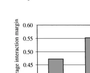
Fig. 8. In#uence of the workload balance on the interaction margin.
processing steps, which &"t in' easily, compensate for the jobs with many processing steps, which are
more di$cult to schedule. The net e!ect of the
variation in the number of processing steps is there-fore small.
The in#uence of the variation in the processing
times is shown by Fig. 6. We observe that higher variation in the processing times results in a higher
average interaction margin. The in#uence of the
overlap on the interaction margin is shown by Fig. 7. We observe that the interaction margin is higher for an overlap of 0 than for an overlap of 1. This is in line with our expectation, because the smaller the overlap the longer the job completion time. However, an average overlap of 0.5 results in the highest average interaction margin, suggesting increased scheduling complexity for these job struc-tures. We further observe that the variation in the
overlap hardly in#uences the interaction margin.
Both center bars in the"gure represent an average overlap of 0.5, with di!erent variation.
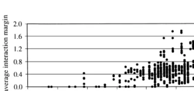
The in#uence of the workload balance on the
interaction margin is given in Fig. 8. This is
repre-sented by a scatter plot, because the workload balance is a random factor. We observe that on average, the interaction margin increases with an increase in the workload balance. This corresponds with our intuition, because a high workload bal-ance means that resource types all have an equal workload. Hence, all resource types have become bottlenecks.
Figs. 4}8 indicated the in#uence of the di!erent interaction factors. An analysis of variance is
per-formed to determine the contribution of the di!
er-ent factors to the explanation of the variability in
the interaction margin. Main e!ects and two-way
interactions are included. The results are given in
Table 6. The results show that all main e!ects,
except for the standard deviation of the number of parallel resources and the overlap, are signi"cant. In addition, several two-way interactions are
signif-icant. Together, the signi"cant factors explain
a large part (91%) of the variability in the interac-tion margin. The proporinterac-tion of the variability in the interaction margin that is accounted for by variation in the interaction factors is given in the last column. The residual plots do not provide reasons for concern. Considering these results, we
conclude that we have identi"ed the most
impor-tant aggregate job set characteristics that are required to predict the interaction.
The experimental results show that some factors
have a stronger in#uence on the interaction margin
than others. The most important variables are:
1. k
!: average number of parallel resources,
2. k
s: average number of processing steps,
3. p
p: standard deviation in processing time, and
4. k
g: average overlap.
In addition, we also include the workload bal-ance (o
.!9) in our further analysis, because in the
experiments we have generated job sets that all had a high workload balance. Therefore, we have
con-sidered mostly values foro
.!9 that are close to 1.
For all other interaction factors, we have con-sidered a wide range of values. We expect that the in#uence of o
.!9 becomes considerably stronger if
a wider range of values is considered. It seems reasonable to include the workload balance in further analysis, because we have encountered
a wider range of values foro
Table 6
ANOVA results for complete model
Sum of squares Degrees of freedom Mean square F-statistic P-value
k
! 1.520 2 0.760 71.0 0.00
p
! 0.007 1 0.007 0.7 0.42
ks 0.502 2 0.251 23.4 0.00
ps 0.132 2 0.066 6.2 0.00
kg 4.966 2 2.483 231.8 0.00
pg 0.029 1 0.029 2.7 0.10
pp 0.916 1 0.916 85.5 0.00
k
!)ks 0.042 4 0.010 1.0 0.42
k
!)ps 0.045 4 0.011 1.1 0.38
k
!)kg 2.346 4 0.586 54.8 0.00
k
!)pg 0.033 2 0.016 1.5 0.22
k!)pp 0.013 2 0.006 0.6 0.55
p!)ks 0.007 2 0.004 0.3 0.71
p!)ps 0.010 2 0.005 0.4 0.64
p
!)kg 0.030 2 0.015 1.4 0.25
p
!)pg 0.000 1 0.000 0.0 0.88
p
!)pp 0.003 1 0.003 0.3 0.60
ks)kg 4.338 2 2.169 202.5 0.00
ks)pg 0.000 1 0.000 0.0 0.89
ks)pp 0.816 2 0.408 38.1 0.00
ps)kg 0.102 4 0.025 2.4 0.05
ps)pg 0.010 2 0.005 0.5 0.62
ps)pp 0.146 2 0.073 6.8 0.00
kg)pp 2.636 2 1.318 123.1 0.00
pg)pp 0.021 1 0.021 2.0 0.16
o
.!9 2.252 34 0.066 6.2 0.00
Error 5.805 542 0.011
Corrected total 84.429 627
Table 7
ANOVA results for reduced model
Sum of squares Degrees of freedom Mean square F-statistic P-value
k
! 1.811 2 0.906 77.5 0.00
ks 1.045 2 0.523 44.7 0.00
kg 12.678 2 6.339 542.1 0.00
p
p 1.021 1 1.021 87.3 0.00
k
!)ks 0.149 4 0.037 3.2 0.01
k
!)kg 2.551 4 0.638 54.5 0.00
k
!)pp 0.022 2 0.011 1.0 0.39
ks)kg 6.719 2 3.360 287.3 0.00
ks)pp 0.754 2 0.377 32.2 0.00
kg)pp 4.487 2 2.243 191.8 0.00
o
.!9 2.312 34 0.068 5.8 0.00
Error 6.666 570 0.012
When the analysis of variance is repeated with only these"ve variables and second-order
interac-tions between these variables included, an R2 of
0.89 is obtained. Table 7 gives the results for the reduced model. Considering these results, we con-clude that a large part of the variability of the interaction margin is explained by only a limited number of interaction factors. All other signi"cant factors and two-way interactions make small con-tributions.
7. Conclusions and directions for further research
In this paper, we studied multipurpose batch process industries with overlapping processing steps, parallel resources and no-wait restrictions between processing steps. We have proposed a method to estimate the feasibility of completing
a job set within a speci"c length of time. The
method is based on predicting job set makespan using aggregate characteristics of the job set. A lower bound on the makespan can be computed easily by considering the workload on the re-sources. Because of job interaction, the minimal makespan for which a feasible schedule is realized will often be larger than the lower bound. Interac-tion at the scheduling level results from relaInterac-tions
between capacity requirements on di!erent
re-sources and from scarcity of capacity.
In this paper, eight factors have been selected to investigate how this interaction margin is deter-mined. These interaction factors are:
1. average number of parallel resources,
2. standard deviation of the number of parallel resources,
3. average number of processing steps per job, 4. standard deviation of the number of processing
steps per job,
5. average overlap of processing steps,
6. standard deviation of the overlap of processing steps,
7. workload balance of resource types, and 8. standard deviation of the processing time.
Experiments in which each of these factors, ex-cept for the workload balance, were varied on two or three levels showed that most factors have a
signi"cant in#uence on the interaction factor. The standard deviation of the number of parallel re-sources was the only main e!ect that was not signif-icant. Furthermore, several two-way interactions proved to have a signi"cant in#uence on the inter-action margin. Together these factors explain 91% of the variation in the interaction margin. Some of these factors have a much higher contribution to the explanation of the variability in the interaction margin than others. The average number of parallel resources, the average number of processing steps, the standard deviation in the processing times, the average overlap and the workload balance are the most important factors.
The experimental results provide a basis for fur-ther development of the prediction model. The pre-diction model may be used to support customer order acceptance decisions. Namely, for a given job set the makespan can be predicted by using the lower bound and the interaction margin for the job set. Orders can be accepted for a period until the expected makespan exceeds the length of the peri-od. The main advantage of this approach is that realistic order sets are obtained for each time
peri-od with small computational e!orts.
Acknowledgements
The detailed comments on earlier versions of this paper by one of the anonymous referees consider-ably improved its clarity and exposition.
References
[1] W.H.M. Raaymakers, J.A. Hoogeveen, Scheduling multi-purpose batch process industries with no-wait restrictions by simulated annealing, European Journal of Operational Research 126 (1) (2000) 131}151.
[2] T.E. Vollmann, W.L. Berry, D.C. Whybark, Manufactur-ing PlannManufactur-ing and Control Systems, 4th Edition, McGraw-Hill, New York, 1997.
[3] J.W.M. Bertrand, J.C. Wortmann, J. Wijngaard, Produc-tion Control: A Structural and Design Oriented Approach, Elsevier, Amsterdam, 1990.
[5] S. Eilon, I.G. Chowdhury, Due dates in job shop schedul-ing, International Journal of Production Research 14 (1976) 223}237.
[6] J.K. Weeks, A simulation study of predictable due-dates, Management Science 25 (1979) 363}373.
[7] K.R. Baker, J.W.M. Bertrand, An investigation of due-date assignment rules with constrained tightness, Journal of Operations Management 1 (1981) 109}120.
[8] K.R. Baker, J.W.M. Bertrand, A comparison of due-date selection rules, AIIE Transactions 13 (1981) 123}131. [9] J.W.M. Bertrand, The e!ects of workload dependent
due-dates on job shop performance, Management Science 29 (1983) 799}816.
[10] M.M. Vig, K.J. Dooley, Dynamic rules for due-date as-signment, International Journal of Production Research 29 (1991) 1361}1377.
[11] M.M. Vig, K.J. Dooley, Mixing static and dynamic# ow-time estimates for due-date assignment, Journal of Opera-tions Management 11 (1993) 67}79.
[12] G.L. Ragatz, V.A. Mabert, A simulation analysis of due date assignment rules, Journal of Operations Management 5 (1984) 27}39.
[13] D.C. Montgomery, E.A. Peck, Introduction to Linear Re-gression Analysis, Wiley, New York, 1992.