Self-sustained amplification of disturbances in pipe Poiseuille flow
L. Bergström
Department of Mathematics, Luleå University of Technology, 97187 Luleå, Sweden
(Received 24 March 1998; revised 10 September 1998; accepted 18 September 1998)
Abstract – The nonlinear development of disturbances in pipe Poiseuille flow is studied with a low-dimensional model. The basic system from which the
model is derived governs disturbances closely related to the radial velocity and radial vorticity disturbances. The analysis is restricted to the interaction of the two first harmonics of streamwise elongated disturbances since they are the most transiently amplified ones in linear theory. In the resulting dynamical system a nonlinear feedback from the normal vorticity disturbance (which is transiently amplified according to linear theory) to the radial velocity disturbance is present. Above a threshold of the initial amplitude, the feedback leads to a self-sustained amplification of the disturbances continuing for all times.Elsevier, Paris
1. Introduction
In 1883 Osborne Reynolds made the remarkable discovery of the transition from laminar to turbulent flow in a circular pipe [1]. The transition occurred if the Reynolds number(R)exceeded a certain value. To explain the transition has since been one of the major efforts in fluid mechanics research. In a number of subsequent experiments by, for example, Wygnanski and Champagne [2], Wygnanski et al. [3] and Fox et al. [4], the lowestR(based on the centerline velocity and the pipe radius) for transition is found to be about 2000–2200.
For a fully developed parabolic mean velocity profile, no theoretical explanation of the transition was ever found in classical stability analysis of the linearized eigenvalue problem. In studies of axisymmetric disturbances by Pekeris [5], Corcos and Sellars [6] and Davey and Drazin [7], only damped modes were found. Herron [8] finally derived a formal proof of stability in the axisymmetric case. For angular dependent disturbances no formal proof of stability exists but from extensive numerical studies by, for example, Lessen et al. [9] and Salwen et al. [10] also angular dependent disturbances are believed to be stable. For finite amplitude disturbances the axisymmetric case was studied by Davey and Nguyen [11], Itoh [12] and Davey [13] but the lack of a neutral stability curve has made the use of expansion techniques difficult and not without controversy. In numerical simulations of finite-amplitude axisymmetric disturbances [14] however, only decaying solutions were found.
The failure of traditional stability analysis to predict the instability has focused interest on alternative mechanisms not based on the classical concept of stability. Such a mechanism is the transient growth mechanism. This mechanism admits a large amplification of small disturbances because of the non-normal properties of the equations governing the disturbances, i.e. the eigenmodes are not orthogonal. In planar flow cases the transient mechanism has been studied by, for example, Farrell [15], Gustavsson [16], Butler and Farrell [17] and Reddy et al. [18].
transiently amplified solution was suggested to provide amplification despite the linear stability. Bergström [20] analytically considered transient growth of small angular dependent disturbances without a streamwise dependence (streamwise wavenumberα=0) and found an amplification of the streamwise disturbance energy density proportional toR2. For the general case of disturbances with an arbitrary streamwise dependence, the
optimal transient growth was studied by Bergström [21] and Schmid and Henningson [22]. The disturbances of the largest amplification were found to be those without a streamwise dependence and with an azimuthal periodicity of unity.
In experiments on transient growth in pipe flow by Bergström [23,24], the transient behaviour of the streamwise disturbance velocity at subcritical Reynolds number was verified. The propagation velocities of the disturbances also agreed with the propagation velocities found analytically by Bergström [21] for the most amplified disturbances.
Although the linear transient mechanism theoretically gives a large disturbance amplification, the distur-bances eventually decay. Therefore, if the transient growth mechanism is a prerequisite for transition some nonlinear mechanism must be involved in addition to it. Boberg and Brosa [19] suggested that the role of nonlinearity is to support the transient mechanism indicated in their simulations by transforming part of the amplified solution into the decaying solution and thereby continually restarting the linear transient process. Subsequently, a number of low-dimensional ad hoc models for shear flows have been presented, where a linear non-normal operator combined with nonlinearity results in a sustained disturbance amplification above some threshold of the initial amplitude. There has been a debate whether nonlinear feedback occurs for a real flow case or not and different routes to transition have been suggested in the models. However, Baggett and Tre-fethen [25] have compared the different models and they assert that the different ideas correspond more closely than it may at first appear. The question of nonlinear feedback will be discussed later in this paper.
In the present paper, a nonlinear low-dimensional model is derived from the equations governing the disturbance development in pipe Poiseuille flow. The motive of the study is to investigate whether a low-dimensional model of disturbances in pipe Poiseuille flow admits sustained amplification. In Section 2 the governing equations for three-dimensional disturbances in pipe Poiseuille flow are given and the model is derived. By exclusively considering the nonlinear interaction of the first modes of the two first harmonics, a dynamical system of eight equations governing the time-development of the disturbances results. In Section 3 the time development of the disturbances and threshold amplitudes for sustained amplification are presented. Finally, in Section 4, the results are discussed and summerised.
2. The governing equations
Consider incompressible viscous flow through a circular pipe. In a cylindrical (x, r, θ ) coordinate system with a laminar mean flowU=1−r2 in the streamwise direction (x), the development of three-dimensional
velocity disturbances(u, v, w)and the associated pressurepis governed by the Navier–Stokes equations
and continuity
In Eqs (1)–(3), all quantities are made dimensionless by the pipe radius and the mean flow centerline velocity,
Ris the Reynolds number,∇2is the cylindrical Laplacian and the prime indicates differentiation with respect to
r. Since the flow is periodic in theθ direction and is assumed to be periodic in thexdirection, the disturbances can be expanded in components according to
(u, v, w, p)T =1 where the ∗ denotes the complex conjugate, α is the streamwise wavenumber and m (integer) indicates the periodicity. A more general form of ansatz for the streamwise and azimuthal dependence has been
P
m
P
nei(mαx+nθ ). However, for the purpose of this work, the form (4) will be more convenient. Also, in (4)
m6=0 is assumed, since only such disturbances will be considered here. By eliminating the pressure in the original equations, the problem can be described by two equations which govern quantities related to the radial velocity disturbance and the radial vorticity disturbance (see, e.g. [22,26]). By introducing
m(t, r)=
the nonlinear versions of the equations governing8mandmare given by
respectively, where the superscript (m) indicates nonlinear terms of periodicity mand where the operators T
The problem is now completely described bymand8msinceumandwmin the nonlinear terms are expressed
inmand8mthrough the relations
um= −
The boundary conditions to be satisfied bymand8mare
• atr =1:
From linear theory it is known thatα=0 disturbances exhibit the largest transient amplification owing to non-normality. However, for pureα=0 disturbances, the disturbance which is transiently amplified (according to linear theory) does not affect the forcing disturbance through nonlinearity (see [27]). The present study of the nonlinear development of the disturbances will therefore be focused on disturbances highly (but not infinitely) elongated in the streamwise direction. Specifically, the linear parts of the governing equations are approximated by theirα=0 form, while in the nonlinear terms,αwill satisfy 0< α≪1. The use of theα=0 version of the linear part of the equations is justified since the transient linear disturbance development for
α≪1 is well represented by the development ofα=0 disturbances. The linearα-terms modify only slightly the linear transient growth ifαis small while the nonlinearα-terms are crucial for a possible nonlinear feedback and sustained amplification. Typically, the magnitude ofα will be of some hundredth-parts which then makes
αR≫1 forR values of practical interest for transition in pipe Poiseuille flow (i.e.R&2000).
The work will from now be focused on a low-dimensional model for the disturbance development and only the nonlinear interaction of the two first components, i.e.m=1 andm=2, which are the most amplified ones in linear theory for smallα, will therefore be considered. Each component can in general be represented as an infinite set of modes with time-dependent coefficients. Here, the eigenmodes associated with the linear and homogeneousα=0 forms of (7a)–(7b) will be exploited. Also, for eachmjust the first mode of8m and the
first mode ofmwill be included in the final model. It should be pointed out that forα=0 disturbances, the
largest contribution to the transient growth comes from the first (and least damped) modes of8mandm. For
largerα, the major contribution comes from the modes at the intersection of the eigenvalue branches (and not from the least damped modes). The dominance of the first modes forα =0 will be further substantiated in Section 3. It should also be emphasized that it is the combination of the modes of8m andmthat causes the
transient amplification.
Forα=0, the eigenmodes are analytically accessible and the first modes of8mandmare given by
and
ωm(r)=Jm(jm,1r), (11b)
respectively, wherejm,1andjm+1,1are the first zeros of the Bessel functionsJmandJm+1, respectively. In a first
mode model ofm=1 andm=2 components,m, 8m, ∗mand8∗mare then decomposed into time dependent
and radially dependent parts according to
8m=am(t)φm(r), 8∗m=a
With (12) inserted into Eqs (7a)–(7b) and by exclusively considering ei(αx+θ ) and e2i(αx+θ ) terms, four
equations are obtained. The equations governing8mandmare then multiplied byJm(jm+1,1r)andJm(jm,1r),
respectively, and then integrated R1
0 ..r dr. By separating the real and imaginary parts of the four radially
integrated equations, a system of eight equations governing the real and imaginary parts of a1, a2, b1 and
b2 (denoted a1r, a1i, a2r, a2i, b1r, b1i, b2r and b2i) results. After some manipulations, the dynamical system
governing the time-development of the disturbances is formally given by
da1r
where the coefficientsℓ1, ℓ2andξ1–ξ10 are radially integrated terms for which the numerical values are given
in the Appendix. The terms containingℓ1andℓ2are the forcing terms causing the transient amplification of
in linear theory. Except forξ1andξ5all otherξ’s depend onαsinceα cannot be factored out from them. (The
In view of the question whether or not nonlinear feedback occurs, the presence of nonlinear-terms in the
8-equations deserves some comment. In plane Poiseuille flow, Benney and Gustavsson [28] and Shanthini [29] have shown that the nonlinear terms of the equation governing the normal velocity (v) do not contain the transiently amplified normal vorticity (η) if oblique disturbances of the formeim(αx+βz)are considered (αandβ
are streamwise and spanwise wavenumbers). If instead for example a pair of oblique disturbances of the form
ei(αx±βz) are studied the situation becomes different and nonlinear terms containing ηoccur in the equation
governingvand thus there is a potential for a nonlinear feedback fromηtov. In a turbulent flow case, Waleffe et al. [30] investigated the different types of nonlinear terms for the particular case of a direct resonance between
vandη. They hypothesized that the dominant regeneration process is a result of the nonlinear self-interaction of thev-terms and that the nonlinearη-terms are small. However, the direct resonance involves higher modes of larger damping which suggests that only a small growth ofη is possible compared to the amplifications obtained from the general transient growth mechanism. For example, in the case of disturbances on a laminar mean flow, Gustavsson [16] reported an induced energy density amplification of 177.9 times for R=1000 owing to the general transient mechanism. The corresponding value for a direct resonance was 16.5 times.
In pipe Poiseuille flow, the form of (13) implies that it is sufficient to exploit the ansatzeim(αx+θ ) to obtain
nonlinear-terms in the8-equations and it is not necessary to use the more general ansatzP
m
P
nei(mαx+nθ ).
However, just the presence of nonlinear -terms does not automatically imply that the feedback is of importance. The subsequent analysis has to reveal whether the feedback in (13) effects the development, i.e. does it counteract or support the establishment of a sustained amplification in pipe Poiseuille flow? Naturally, the model (13) is a very simplified model where for example no generation of higher components is included. It cannot be expected that a very complex phenomenon like laminar-turbulent transition can be fully described by a model like (13). However, in spite of the simplicity, if the full basic equations governing the stability of pipe Poiseuille flow allow a sustained disturbance amplification, the transition may also be indicated by a low-dimensional model derived from the basic equations.
The system (13) is solved numerically by a 4th and 5th order Runge–Kutta–Fehlberg integration method. The resulting disturbance development is characterized by the energy density of the disturbances defined by
Em=π
normalized by the initial energy density denoted Em0. The initial disturbance is defined by giving a1r and
a1i equal values (all the others are zero initially) and the parameter ε=a1r =a1i is used to define the initial
disturbance strength.
3. Results
3.1. The time development of the disturbances
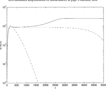
In figure 1 the development ofE1/E10 is presented forR=4000, α=0.03 andε=0.004 (dashed dotted),
ε=0.0079 (dashed) and ε=0.008 (solid). For ε=0.004, the development is as in the linear case, i.e. the disturbance is transiently amplified to a peak and then decays. The peak occurs att=198 and the maximum amplification is 1075. In spite of the few modes included in the model (13), these values coincide well with the values found in linear studies ofα=0 disturbances where the peak position occurs att/R≃0.049 and the optimal amplification forR=1000 isE1/E10≃72. WithR=4000, the corresponding values aret=196
Figure 1. Development ofE1/E10forR=4000, α=0.03, ε=0.004 (dashed dotted),ε=0.0079 (dashed) andε=0.008 (solid).
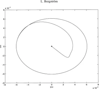
case ε=0.0079, the disturbance does not start to decay immediately after the linear peak is reached as in the previous case. Here, nonlinearity has an influence and the amplification is maintained for a substantially longer period until the decay rate finally increases and the disturbance rapidly decays. With ε=0.008, the disturbance behaves at first as in the previous case untilt≃700. Then it becomes further amplified to about 2.3 times the linear maximum amplification and a sustained state of amplification continuing for all times becomes established. Although the model (13) solely describes the nonlinear development of disturbances highly elongated in the streamwise direction, the results indicate that the linear transient growth combined with nonlinearity is capable of causing a sustained amplification of disturbances in pipe Poiseuille flow. For the same values of parameters as in the sustained case presented in figure 1, the phase-plane development of
b1r versus b1i from (13) is presented in figure 2. The calculations are performed for 06t6100·103 and
the star indicates the initial point. Initially, owing to the choice of initial disturbance, b1r and b1i are zero.
After a while, the trajectory follows a fixed track and the sustained state of amplification is represented by a limit cycle of circular shape. (The same behaviour is obtained for other pairs of (13)). As a consequence, since for exampleE1/E10 depends ona21r +a21i and b21r+b21i, the energy density becomes constant although
the individual components of (13) oscillate. Although it is not formally proven that the sustained amplification continues for all times, the result showing a sustained limit cycle fort up to 100·103makes this plausible.
Figure 2. Phase-plane development ofb1rversusb1iforε=0.008, α=0.03, R=4000 and 06t6100·103.
3.2. Threshold amplitudes ofεfor a sustained amplification
From numerical tests, the threshold (i.e. the lowest value) of ε for a sustained amplification versus the correspondingRis presented in figure 3a forα=0.03 (cross),α=0.05 (star) andα=0.1 (circle). The curves are displaced towards largerRasαdecreases and the threshold amplitude for sustained amplification begins to be relatively high for values ofR below some thousands. In addition, forα≪1 and lowerR(but stillαR≫1, for example, α=0.03 andR =1000), it can be pointed out that no sustained state has been obtained. For largerαand lowerR, sustained amplification can be achieved but the requirement thatα≪1 in the derivation of the model becomes violated. In figure 3b the threshold amplitude ofεversus the corresponding value ofRis presented in a logarithmic diagram forα=0.03 (solid),α=0.05 (dashed) andα=0.1 (dashed dotted). With an assumed threshold relation of the formε=constantRg, all curves in figure 3b indicate unambiguously that
g= −3. In the next section, the indicated value ofgwill be explained by a heuristic consideration of Eq. (13). It can be mentioned that in some tests withεwell beyond the lowestεfor sustained amplification, the solution may decay for a narrow interval ofε and then again become sustained outside the interval. This observation has been made close to the lowestRfor which sustained solutions have been achieved for a certainα.
4. Discussion and conclusion
(a)
(b)
Figure 3. (a) Numerically obtained threshold amplitudes ofεfor sustained amplification versus the Reynolds numberR.α=0.03 (cross),α=0.05 (star) andα=0.1 (circle). (b) Logarithmic diagram of the threshold amplitude ofεversus the corresponding value ofRforα=0.03 (solid),α=0.05
theory. The results show that a self-sustained disturbance amplification occurs. Concerning the feedback and the importance of different types of nonlinear terms, tests with thebb-terms switched off in the a-equations (13a)–(13d) have been performed. In all such tests the disturbance decays after the transient phase and no sustained state is established for the same parameter values that give sustained amplification if thebb-terms are included. Also, of course, if the linear forcing terms (ℓ1andℓ2) in (13e)–(13h) that cause the transient growth
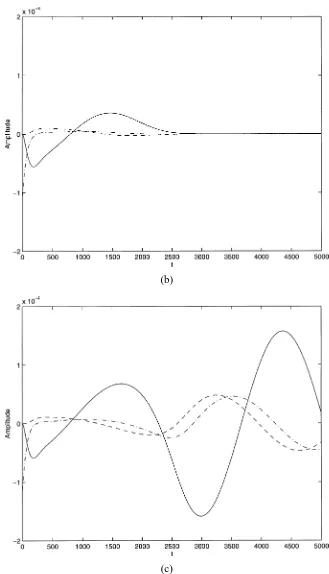
of theb-terms are switched off, no amplification or sustained state occur. In figures 4a–c the nonlinearbb-term (solid),ab-term (dashed) andaa-term (dashed dotted) from Eq. (13c) are presented. The parameter values are
R=4000, α=0.03, ε=7.5·10−3(4a),ε=7.75·10−3(4b) andε=8.0·10−3(4c). The values ofεare here
just below the threshold amplitude in 4a and 4b and just above the threshold amplitude in 4c. In all three cases the traces of theaa-terms (dashed dotted) andab-terms (dashed) are quite similar untilt≈2500. Concerning thebb-term (solid), the first negative period is very similar in the three cases but in the subsequent positive period the peak amplitude becomes approximately twice as large each timeε is increased. After the positive phase of larger amplitude of thebb-term in figure 4c, also theaa- andab-terms change behaviour and start to oscillate. Roughly speaking, one can say that when thebb-term goes positive, theaa-term andab-term tend to go negative and vice versa. The nonlinear terms ofa2i exhibit a similar behaviour. Fora1r anda1i the situation
is different and apart from the sign, the magnitude of the nonlinear terms are more equal. The conclusion from
figures 4a–c is that close to the threshold amplitude, the significant changes of the nonlinear terms in (13c)
are related to thebb-term for which the positive peak amplitude increases substantially when ε is increased in the neighbourhood of the threshold amplitude. There thus exists a nonlinear feedback from the transiently amplified disturbanceto the forcing disturbance8. Above a threshold of the initial disturbance amplitude, the feedback causes a sustained disturbance amplification continuing for all times.
In figure 3b the threshold relation ε∼R−3is indicated. The obtained exponent g= −3 can be understood by a heuristic consideration of Eq. (13) similar to the one done by Baggett and Trefethen [25]. If thebb-term is
(b)
(c)
assumed to be important at the stage when the disturbance becomes sustained, a simple heuristic model of the nonlinear development of, for example,a2r in (13c) owing to theb1rb1i-term is
da2r
dt + j3,12
R a2r ≈2ξ5R
2α2b
1rb1i, a2r(0)=0 (15)
whereξ5is independent ofα andR as explained earlier. Ifb1r andb1i are approximated byε, the solution of
(15) is
a2r(t)≈2ξ5
R3α2ε2
j3,12
1−e(−j3,12 /R)t. (16)
To achieve a sustained process, one can demand thata2r ≈ε after a long period of time. Thus (16) implies
a threshold relation ε ∼α−2R−3. (Another simple interpretation is just that the b
1rb1i-term should be able
to overcome the damping term ((j3,12 /R)a2r). The heuristic analysis makes the numerically obtained value
g= −3 reasonable. The exponent −3 is the same as obtained in several of the suggested low dimensional ad hoc models for transition which are compiled in [25]. From experimental results for pipe Poiseuille flow published by Darbyshire and Mullin [32], Baggett and Trefethen [25] suggested an exponent below−1, perhaps in the vicinity of−1.5. In relation to that value, the exponent indicated by the model (13) is then too low. It is reasonable to ascribe the discrepancy to the simplicity of the model exploited here. The model consists solely of smallα components which are the most transiently amplified ones according to linear theory. The model therefore favours the transient part of the development. In reality a broad range of components are of course involved in the transition process. The generation of higher harmonics and more general structures are absent in a low-dimensional model like (13). An improved model containing more components which are less transiently amplified thanα=0 components should possibly change the behaviour but also grow in complexity and become less tractable.
Although the present model is a low-dimensional one of streamwise elongated disturbances and should just be considered as a contribution to the debate, the obtained results indicate that the transient growth mechanism in combination with nonlinear feedback is capable of causing a state of permanent amplification of disturbances in pipe Poiseuille flow. The model is derived from the basic equations of a real flow case and incorporates the initial growth mechanism for small disturbances on a parabolic mean flow as well as the establishment of a self-sustained process. Moreover, although the full nonlinear problem and the transition phase are high-dimensional and include a broad range of wave components and modes, the basic self-sustaining process may essentially be related to low wave number components since they are the most transiently amplified and less damped ones.
Appendix
The coefficients of the system (13) have the following numerical values:
j1,1=3.83171, j2,1=5.13562, j3,1=6.38016,
ℓ1= −0.99294, ℓ2= −0.24283,
ξ1=0.04752, ξ2= −0.00793, ξ3=0.00172, ξ4= −0.42386, ξ5=0.02942,
Except forξ1 and ξ5 which are independent ofα, the values of the ξ’s are for α=0.03. Observe that the
coefficientsξ1, ξ2, ξ3, ξ5andξ6of the nonlinear terms containingbin thea-equations (13a)–(13d) are closer to
zero than the coefficientsξ4andξ7of the nonlinear terms containing solelya terms in (13a)–(13d). However,
since the nonlinear terms containing b in (13a–d) are multiplied byα2R2 orR, they have potential to reach the same magnitudes as the nonlinear terms containing solely a’s. This is substantiated in Section 4 and in
figures 4a–c.
References
[1] Reynolds O., An experimental investigation of the circumstances which determine whether the motion of water shall be direct or sinuos, and the law of resistance in parallel channels, Philos. T. Roy. Soc. London 174 (1883) 935–982.
[2] Wygnanski I.J., Champagne F.H., On transition in a pipe. Part 1. The origin of puffs and slugs and the flow in a turbulent slug, J. Fluid Mech. 59 (1973) 281–335.
[3] Wygnanski I.J., Sokolov M., Friedman D., On transition in a pipe. Part 2. The equilibrium puff, J. Fluid Mech. 69 (1975) 283–304. [4] Fox J.A., Lessen M., Bhat W.V., Experimental investigation of the stability in Hagen–Poiseuille flow, Phys. Fluids 11 (1) (1968) 1–4. [5] Pekeris C.L., Stability of the laminar flow through a straight pipe of circular cross-section to infinitesimal disturbances which are symmetrical
about the axis of the pipe, Proc. U.S. Nat. Acad. Sci. 34 (1948) 285–294.
[6] Corcos G.M., Sellars J.F., On the stability of a fully developed flow in a pipe, J. Fluid Mech. 5 (1959) 97–112. [7] Davey A., Drazin P.G., The stability of Poiseuille flow in a pipe, J. Fluid Mech. 36 (1969) 209–218.
[8] Herron I., Observations of the role of vorticity in the stability of wall bounded flows, Stud. Appl. Math. 85 (1991) 269–286. [9] Lessen M., Sadler S.G., Liu T.-T., Stability of pipe Poiseuille flow, Phys. Fluids 11 (1968) 1404–1409.
[10] Salwen H., Cotton F.W., Grosch C.E., Linear stability of Poiseuille flow in a circular pipe, J. Fluid Mech. 98 (1980) 273–284. [11] Davey A., Nguyen H.P.F., Finite-amplitude stability of pipe flow, J. Fluid Mech. 45 (1971) 701–720.
[12] Itoh N., Nonlinear stability of parallel flows with subcritical Reynolds numbers. Part 2. Stability of pipe Poiseuille flow to finite axisymmetric disturbances, J. Fluid Mech. 82 (2) (1977) 469–479.
[13] Davey A., On Itoh’s finite amplitude stability theory for pipe flow, J. Fluid Mech. 86 (1978) 695–703.
[14] Patera A.T., Orszag S.A., Finite-amplitude stability of axisymmetric pipe flow, J. Fluid Mech. 112 (1981) 467–474. [15] Farrell B.F., Optimal excitation of perturbations in viscous shear flow, Phys. Fluids 31 (8) (1988) 2093–2102.
[16] Gustavsson L.H., Energy growth of three-dimensional disturbances in plane Poiseuille flow, J. Fluid Mech. 224 (1) (1991) 241–260. [17] Butler K.M., Farrell B.F., Three-dimensional optimal perturbations in viscous shear flow, Phys. Fluids A 4 (8) (1992) 1637–1650. [18] Reddy S.C., Schmid P.J., Henningson D.S., Pseudospectra of the Orr–Sommerfeld operator, SIAM J. Appl. Math. 53 (1) (1993). [19] Boberg L., Brosa U., Onset of turbulence in a pipe, Z. Naturforsch. A 43a (1988) 697–726.
[20] Bergström L., Initial algebraic growth of small angular dependent disturbances in pipe Poiseuille flow, Stud. Appl. Math. 87 (1992) 61–79. [21] Bergström L., Optimal growth of small disturbances in pipe Poiseuille flow, Phys. Fluids A 5 (11) (1993) 2710–2720.
[22] Schmid P.J., Henningson D.S., Optimal energy density growth in Hagen–Poiseuille flow, J. Fluid Mech. 277 (1994) 197–225. [23] Bergström L., Evolution of laminar disturbances in pipe Poiseuille flow, Eur. J. Mech. B-Fluid. 12 (6) (1993) 749–768.
[24] Bergström L., Transient properties of a developing laminar disturbance in pipe Poiseuille flow, Eur. J. Mech. B-Fluid. 14 (5) (1995) 601–615. [25] Baggett J.S., Trefethen L.N., Low-dimensional models for subcritical transition to turbulence, Phys. Fluids 9 (4) (1997) 1043–1053. [26] Burridge D.M., Drazin P.G., Comments on “Stability of pipe Poiseuille flow”, Phys. Fluids 12 (11) (1969) 264–265.
[27] Bergström L., Nonlinear behaviour of transiently amplified disturbances in pipe Poiseuille flow, Eur. J. Mech. B-Fluid. 14 (6) (1995) 719–735. [28] Benney D.J., Gustavsson L.H., A new mechanism for linear and nonlinear hydrodynamic instability, Stud. Appl. Math. 64 (1981) 185–209. [29] Shanthini R., On the nonlinear development of small three-dimensional perturbations in plane Poiseuille flow—a single mode approach, Stud.
Appl. Math. 84 (1991) 93.
[30] Waleffe F., Kim J., Hamilton J.M., On the origin of streaks in turbulent shear flows, in: Durst F., Friedrichs R., Launder B.E., Schmidt F.W., Schumann U., Whitelaw J.H. (Eds.), Turbulent shear flows 8, Springer, Berlin, 1993, pp. 37–49.