*Corresponding author. Tel.:#1-773-702-7513; fax:#1-773-702-2857.
E-mail address: [email protected] (P.E. Rossi).
0304-4076/00/$ - see front matter ( 2000 Elsevier Science S.A. All rights reserved. PII: S 0 3 0 4 - 4 0 7 6 ( 0 0 ) 0 0 0 3 4 - 8
A Bayesian analysis of the multinomial probit
model with fully identi"ed parameters
Robert E. McCulloch
!
, Nicholas G. Polson
!
, Peter E. Rossi
!,
*
!Graduate School of Business, University of Chicago, Chicago, IL 60637, USA
Received 5 May 1998; received in revised form 1 December 1999; accepted 25 April 2000
Abstract
We present a new prior and corresponding algorithm for Bayesian analysis of the multinomial probit model. Our new approach places a prior directly on the identi"ed parameter space. The key is the speci"cation of a prior on the covariance matrix so that the (1,1) element if"xed at 1 and it is possible to draw from the posterior using standard distributions. Analytical results are derived which can be used to aid in assessment of the prior. ( 2000 Elsevier Science S.A. All rights reserved.
JEL classixcation: C11; C25; C33; C35
Keywords: Probit models; Bayesian analysis; Priors
1. Introduction
proposed the method of simulated moments and Hajivassiliou and McFadden (1990) have proposed the method of simulated scores (see also Keane, 1994; and Borsch-Supan and Hajivassiliou, 1993).
A Bayesian analysis of the MNP model is given in McCulloch and Rossi (1994) (henceforth MR) (see also Nobile, 1998). The MNP model, as commonly speci"ed, has a vector of coe$cientsband a covariance matrixRas parameters. However, the parameters (b, R) are not fully identi"ed. The model is often identi"ed by setting the"rst diagonal element of the covariance matrix equal to one (p11"1). A key feature of the MR method is the manner in which the identi"cation issue is handled. In the MR approach, a proper prior is speci"ed for the full set of parameters (b, R) and the marginal posterior of the identi"ed parameters (b/Jp11,R/p11) is reported. Thus, the prior on the identi"ed para-meters is the marginal prior of (b/Jp11, R/p11) derived from the prior distribution speci"ed for the full set of parameters (b, R). The approach is taken because of the di$culties associated with a Bayesian analysis of covariance matrices with"rst diagonal element"xed at one. Since it is imposs-ible to specify a truly di!use or improper prior with this approach, the induced priors must be inspected to assure that they properly represent the investigators beliefs.
In this paper, we present a new approach which places a prior directly on the set of identi"ed parameters. We do this by specifying a prior onRsuch that the "rst diagonal element is one with probability one. We discuss both the assess-ment of the prior and the computation of the posterior. Computation of the posterior involves a simple Gibbs sampler in which each draw is either normal, truncated univariate normal, or Wishart. The new prior can be both informative or di!use and improper. We present analytical results that facilitate the prior speci"cation in both the new prior and that of MR. However, we see in the examples that this simple method of achieving identi"cation comes at a cost: the Gibbs sampler produces a Markov chain which tends to be more highly autocorrelated that the Markov chain used in the MR approach. In some extreme cases, the Markov chain for the identi"ed parameter case will fail to converge. These cases occur in high dimensions and in situations in which the likelihood is not very informative.
cause convergence problems. Section 8 discusses the pros and cons of the new approach and brie#y compares it with other approaches in the literature.
2. The multinomial probit model
2.1. The model
In this section we brie#y review the MNP model. Let>be a random variable such that>3M0, 1, 2,2,p!1NandXbe a (p!1)]kmatrix. The conditional distribution of>DXis speci"ed as follows. First, let
="Xb#e, (1) and the model parameters arebandR. Typically in application, we observe a set of observations (>
i, Xi) and assume that given theX's the>'s are independent. Various elaborations of the model have been considered (see for example MR Sections 8 and 9).
At this point, some of the di$culties associated with the analysis of the MNP model may be appreciated. To compute the likelihood we must compute the probability of sets of the formM=D>(=)"iNwhere=&N(Xb, R). The sets are cones inRp~1. Much of the research on the MNP model has been devoted to the development of e$cient computational methods for computing these inte-grals. the MNP model see Dansie (1985), Bunch (1991), and Keane (1992) for example.
Letp
frequentist methods. It is not straightforward to adopt this approach in a Bayesian analysis because of the di$culty in de"ning a prior on the set of covariance matrices such that the (1, 1) element is one.
3. An algorithm with non-identi5ed parameters
3.1. The algorithm
In this section we brie#y review the method developed in MR for a Bayesian analysis of the MNP model. The method uses the full set of parameters (b, R). Because of the model is not identi"ed, we use a proper prior to ensure that the posterior is proper. The prior speci"cation lets b and R be independent with
b having a multivariate normal distribution and G"R~1 having a Wishart distribution:
lare the parameters of the inverted Wishart prior:R~1&W(l, <). Note that our parameterization of the Wishart distribution is such that E(R~1)"l<~1. In practice, we choose values for (bM, A, l,<) and then check that the marginal prior of the identi"ed parameters (b/Jp11, R/p11) is reasonable. Theoretically, our marginal posterior is the same as that obtained by working with just the identi"ed parameters (b/Jp11, R/p11) and the marginal prior on them derived from the prior speci"ed for the full set of parameters. MR uses the full set of parameters so that the following simple algorithm may be used to compute the posterior.
The method uses Gibbs sampling to obtain draws from the posterior distribu-tion. Gibbs sampling is discussed in Gelfand and Smith (1990), Casella and George (1992), Smith and Roberts (1993), and Tierney (1994) among many others. In the Gibbs sampling approach, we sample the =
i in (1) above. As pointed out by Albert and Chib (1993), introducing the latent variablesM=
iNto be drawn in addition to (b,R) greatly simpli"es the algorithm.
Let=
ijbe thejth element of theith=vector. Let=i(~j) be theith=vector with=
ijremoved. Given the dataD"M>i, XiN, the Gibbs sampling algorithm proceeds by drawing from the following set of conditional distributions:
The draw ofbis from a multivariate normal, the draw ofRis from an inverted Wishart distribution, and the draw of each=
ijis a univariate truncated normal. Nobile (1998) has proposed an elaboration of the algorithm above. A Metrop-olis step is added in which the current values of all=,b, andRare scaled up or down by a positive constant and the algorithm jumps to the scaled values or not in the usual Metropolis manner. Nobile provides evidence that this added step signi"cantly improves the performance of the Markov chain.
4. A method with fully identi5ed parameters
In this section, we describe an alternative prior and corresponding Gibbs sampling algorithm for the MNP model. The prior assigns probability one to the setMRD p11"1Nin such a way that we are able to draw fromRD b, M=
iN, D. Thus, our algorithm for computing the posterior will be same as before, except for the draw of R. As discussed in Section 2.2 above, by "xing p11"1, we identify the parameters of the MNP model.
The"rst two draws are just as in MR withRobtained fromc, Uandp11"1. The third draw is a normal and the fourth draw is an inverted Wishart. The exact form of these last two draws is given in the appendix.
5. Analytical results and prior assessment
We shall refer to the approaches of Sections 3 and 4 as NID and ID (not identi"ed and identi"ed), respectively. In this section we present analytical results that help us understand and choose the priors in both approaches.
First some notation. In the NID approach, one dimension of the parameter is unidenti"ed and a proper prior is used to ensure that the posterior is proper. In the ID approach only the identi"ed parameters are used. To clearly distinguish the identi"ed parameters from the `fulla set we shall henceforth refer to the parameters of the NID method as bI and RI. We use b and R to denote the parameters identi"ed by the restrictionp11"1:b"bI/Jp811 andR"RI/p811.
Under the NID prior,bI&N(bM, A~1) andRI~1&W(l,<) so that the set of prior parameters which must be chosen is (bM,A, l, <). Under the ID prior we haveb&N(bM, D~1), c&N(c6, B~1), andU~1&W(i, C) so that the set of prior parameters is (bM, D, c6, B, i, C).
Note that in the ID case we have the option of using the standard improper choices:D"0,B"0, andi"0. In this case the choices ofbM, c6, andCdo not matter. In the NID case we must choose a proper prior.
Both the NID prior and the ID prior have unusual forms. In the remainder of this section we derive results about these non-standard priors and use these results to help us choose the prior parameters. We assume that the prior is assessed, at least approximately, by choosing appropriate marginals forbandR. For both priors, we obtain results about the marginal priors on the identi"ed parametersbandR. We"rst explore the marginal prior ofbin each prior and then that ofR. Proofs of all results are available in the appendix.
5.1. The prior forb
The simplest prior is that ofbin the ID algorithm:b&N(bM,D~1). In the NID approach the prior forb is more complicated. Result 1 below gives the prior distribution of the identi"ed coe$cients using the NID prior. We need the following notation:
<~1"
C
v11 v12v21 <22
D
, (8)wherev11is 1]1,v12is 1](p!2),v21"(v12)@, and<22is (p!2)](p!2). Let
Result 1. Under the NID prior the marginal distribution is b"bI/Jp811& Jv1.2s bI, wheres2&s2l
~p`2 independent ofbI&N(bM, A~1).
Result 1 tells us that the form of the prior forbusing the NID method is quite unusual: the square root of a chi-squared random variable times a normal. When bM is 0, this will result in a distribution with heavy tails relative to the normal. WhenbM is non-zero the distribution will be skewed.
A basic feature of the NID prior is that b and R are not independent. In Result 1, we see that the prior forbdepends on that ofRthroughlandv1.2. The easiest thing to do in practice seems to be to choose the prior forRand then choose that ofb givenlandv1.2.
5.2. The prior forR
In both the ID and the NID case, we assume that as a"rst step in choosing the prior parameters forR, we are able to specify its expected value
E(R)"
C
1 E(c)@E(c) E(U)#E(cc@)
D
"C
1 E(c)@
E(c) D#E(c)E(c)@
D
, (9)whereD"E(U)#<ar(c).
Given E(R), both E(c) andDare known.
5.2.1. The ID case
Our goal is to choose values for the prior parameters (c6, B,i,C) where
c&N(c6, B~1) and U~1&W(i, C). We take as given E(c) and D. Clearly,
c6"E(c). Using a standard result in multivariate analysis we have, E(U)"C/(i!p#1), giving
D" C
(i!p#1)#B~1. (10)
Thus,
C"(i!p#1)(D!B~1). (11)
Consider the simple but important case where we wish to have E(R)"I. Then E(c)"0 andD"I. If we simplify by lettingB~1"qIthen speci"cation of the prior now involves only the choice of the two scalarsi andq! Since i is the degrees of freedom in our inverted Wishart prior,iandqcontrol the tightness of the prior with large values ofiand small values ofqgiving tighter priors. The relative variability of cand Udetermine the prior distribution of the correla-tions. To see this, note that in the case p"3, the single correlation in R is
5.2.2. The NID case
The prior parameters ofRin the NID case are (l,<) where RI~1&W(l,<). Our goal is to have some understanding of the implications of choices for (l,<) on the prior distribution of R"RI/p811. Since (c, U) constitute a one-to-one reparametrization of the identi"edR, our approach is to derive the marginal priors ofcandUgiven choices ofland<.
Result 2. Under the NID prior the marginal distribution of c is multivariate
twithl!p#3 degrees of freedom and
E(c)"(<22)~1v21 and <ar(c)" v1.2
l!p#1 (<22)~1. (12)
Result 3. Under the NID prior the marginal distribution ofU~1is of the form
U~1"=
u where=&Wishart(l, (<22)~1) andu&v1.2s2l~p`2 (13)
with=anduindependent.
From result (3), we have
E(U)"v1.2(l!p#2)
l!p#1 (<22)~1. (14)
To use these results, we again suppose that we are able to specify the expected value of R so that E(c) and D are given. Our results give
D"E(U)#<ar(c)"v1.2(<22)~1(l!p#3)/(l!p#1). Given choices for v1.2 andlwe can obtain (<22)~1fromD. Given (<22)~1, we can obtainv21from E(c). Thus, given E(R) we have only the two numberslandv1.2left to choose in order to specify the prior.
As a simple example we can let (as we did in the ID case) E(c)"0 andD"I. This implies thatv12"0,v1.2"v11and
<22"v11(l!p#3)
(l!p#1) I. (15)
6. Simulated examples
In this section we apply the ID approach to two simulated examples. The examples are the same as those of MR. In the "rst examplep"3 and in the secondp"6.
We consider two versions of the ID prior. In both cases we chooseD"0, an improper choice for the prior onb. In choosing our prior forR, we center the prior on theIso that (as in Section 5.2.1) all we must specify are values foriand
q. In our"rst prior we choose i"p#2 and q"1
8. In our second prior we chooseB"0 and i"0 so that the prior onRis improper as well.
In both priors we avoid making choices about the prior forb. In the"rst prior we have chosen to roughly center our prior forRat the identity matrix. In the second prior we avoid making choices forRas well.
Each run of a Gibbs sampler is started at the initial valuesb"0 andR"I. Since we draw="rst, there is no need to specify initial values.
6.1. Simulated example withp"3
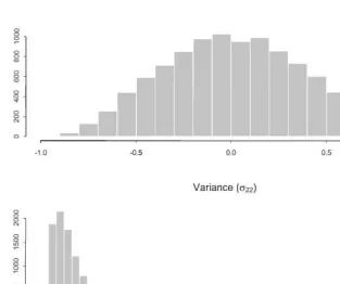
With p"3,R is 2]2 so there is just one unconstrained variance and one correlation. Fig. 1 displays the marginal prior distributions of the single correla-tion (top panel) and the single variance given the choices of the"rst ID prior:
i"(p#2)"5 and q"1
8. The histograms are constructed from 10,000 iid draws from the prior. We see that the prior for the correlation is centered at zero but spreads out towards $1. The prior for the variance has mean one and a long right tail. Of course, we cannot display the any marginal priors for the second prior choice since it is improper on bothbandR.
Data was simulated as follows. The matrix Xhas just one column and the corresponding true value of the single coe$cient equals!1.414. Each of the
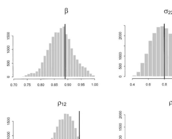
X values was drawn iid from the uniform distribution on the interval (!0.5, 0.5). The true value of the correlation is 0.5 and the true value of the unconstrained variance is 2. Three thousand observations were simulated.
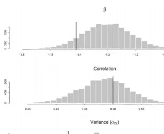
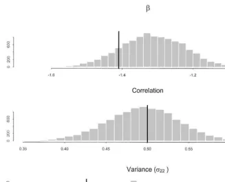
Fig. 2 displays the posteriors of the three parameters (b, p22, and o12) obtained from the"rst choice of ID prior. In each histogram the solid line is drawn at the value of the true parameter. These histograms are based on 10,000 iterations of the Gibbs sampler outlined in Section 4 (after discarding a few initial burn in draws). Fig. 3 displays the results using the second prior (improper onR). The results displayed in Figs. 2 and 3 are very similar and both appear to be quite reasonable.
Fig. 1. ID prior distributions.
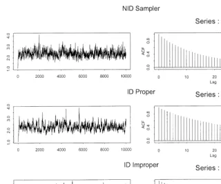
three cases the autocorrelation functions die o!as the lag increases. Clearly, the draws from the ID samplers are more highly autocorrelated than those of the NID. The draws from the ID sampler using the second prior are more highly autocorrelated than those of the"rst. For example, the 10th autocorrelation is 0.77 for the second prior and 0.71 for the"rst.
This example illustrates a basic feature of the Gibbs sampler of Section 4 for the ID prior. The more di!use the prior onRis, the slower the autocorrelations die out. We have tried many simulated examples and found this to be generally true.
6.2. Simulated example withp"6
Fig. 2. Posterior distributions}proper ID prior.
Fig. 5 displays four of the marginal posteriors obtained from our"rst ID prior (i"8, q"1
8). These histograms are based on 30,000 iterations of the Gibbs sampler. Again, in each case the solid line depicts the true value of the para-meter. The top left panel isb, the top right isp22, the bottom left iso12and the bottom right iso23. As in thep"3 case the sampler seems quite successful.
The sampler run using the second prior, which is improper onR, got stuck at a R which was almost singular at about the 15,000th iteration. In the next section we discuss the relationship between the performance of the sampler and the choice of prior.
7. Marginal priors for eigenvalues
The examples of the previous section show the choice of ID prior has an e!ect on the performance of the corresponding Gibbs sampler. In this section, we explain how the prior a!ects the performance of the sampler.
Fig. 3. Posterior distributions}improper ID prior.
may be guiding the sampler to matrices of this type. In order to get a feeling for this we use the smallest eigenvalue as a measure of how close to singularity a particularRmay be. We now examine the prior distribution of the smallest eigenvalue.
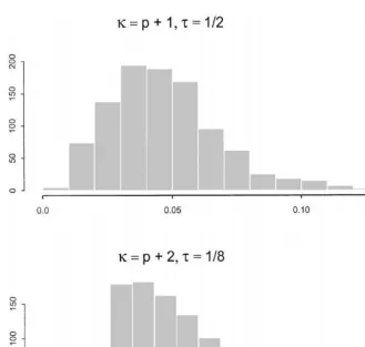
Fig. 6 displays the marginal prior distribution of the smallest eigenvalue of
Rfor two choices of the ID prior in the casep"6 (soRis 5]5). The top panel corresponds to the choicesi"p#1 andq"1
2. The bottom panel corresponds to the choices i"p#2 and q"1
8 used in Section 6. These two priors are markedly di!erent. In the top panel most of the mass is on values less than 0.1 while in the bottom panel most of the mass is on values greater than 0.1. Since the identity matrix has smallest eigenvalue equal to 1, it makes sense that if we tighten up our prior around R"I we will move the marginal prior of the smallest eigenvalue towards 1.
Fig. 4. Time-series properties of NID, ID proper and ID improper samplers.
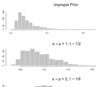
with a very small simulated sample of data and check the posterior for in#uence from this prior. We simulated seven observations from the N
5(0,I) distribution and then computed the posterior ofRgiven these observations. The idea is that the posterior from a small data set will largely re#ect features of the prior. The data set is chosen to be large enough to turn the improper prior into a proper posterior. We then computed the marginalposteriordistribution of the smallest eigenvalue ofR. We did the same thing for the two priors displayed in Fig. 6. The results are displayed in Fig. 7. The top, middle, and bottom panels, correspond to the improper, i"p#1 and q"1
Fig. 5. Posterior distributions of model parameters:p"6 example.
Recall that in thep"3 example the sampler based on the improper prior had no problem.
8. Advantages and disadvantages of ID prior
The NID prior approach is most useful in situations in which a proper but fairly di!use prior is desired. However, the results in Section 5 show that it may be di$cult to assess a truely informative prior onbusing the NID approach. This is particularly true if a prior mean other than zero is desired. In contrast, the ID approach can be used to assess a standard normal prior directly onb. There are a number of situations in which informative priors are desireable. For example, hierarchical models for situations in which the data has a panel or grouped structure have become increasing popular. The heart of the hierarchical model is an informative prior on the coe$cients. Typically, we would assume that each panel memberjcorresponds to a set of coe$cientsbj, and use a prior
bj&N(bM, <
b). (16)
Fig. 6. Prior distributions of smallest eigenvalue.
approach can be extended easily to handle a variety of hierarchical models of this sort.
Informative priors onbare also useful in situations in which the investigator has prior information from subject matter theory or experience with similar datasets. For example, a multinomial model for choices between di!erent brands of similar products as in Nevo (1997) would feature a price coe$cient which is certainly negative and never much less than!20 or so.
Note that this approach to prior speci"cation should be viewed as a way to roughly gauge the prior since we assume that the prior is assessed by separately choosing marginals for b and R. Given the nature of the MNP model, prior information should involve dependence betweenb and R. For example, prior information may be about the implied probabilities rather than directly about
Fig. 7. Posterior distribution of smallest eigenvalue}small dataset.
model (the main competitor to the MNP) it is possible to assess the prior in a more natural way (see Koop and Poirier, 1993). For the more complicated MNP model prior assessment is a di$cult problem. If, for example, the re-searcher had prior information about the underlying utility maximization pro-cess leading to the multinomial data it might be possible to specify a prior on the full set of parameters (bI andRI) and actually use that data to learn about the unidenti"ed parameters (see Poirier, 1998).
problems with a small amount of data. Note that, in practice, is very easy to identify when the sampler is stuck so that there is no possibility of actually reporting incorrect results.
There is an accumulating body of evidence in the statistics literature on covariance matrix estimation that a modest amount of shrinkage on the eigen-values or correlations will produce estimators with good risk properties (see Yang and Berger, 1994; Daniels and Kass, 1999). Thus, an improper prior on
Rhas at least three undesirable aspects: (1) it is actually a very informative prior on the smallest eigenvalue, (2) the sampling properties of Bayes estimators based on this prior are apt to be poor and (3) our ID Gibbs sampler may experience convergence problems with this prior. For these reasons, we advocate the use of a weakly informative default prior onR(centered onI) in the absence of strong prior information. The improper prior onRcan be used as a diagnostic for prior sensitivity, if desired.
Other possible approaches to assessing priors directly on the identi"ed parameters include using the prior of Barnard et al., 2000 (see, also, in McCul-loch and Rossi, 1996) and the approach of Chib et al. (1998). In the Barnard et al. approach,Ris written as Diag(S)RDiag(S) and various priors are used on the standard deviations and correlations. This prior can be implemented in a Griddy Gibbs algorithm since the relevant range of each correlation can be expressed as function of all other correlations, allowing a one-by-one draw of R. The Griddy Gibbs algorithm is reliable but it can be slow and requires the choice of grid size and boundaries. Some additional work would be required to assess truely informative priors on R. Chib et al. (1998) propose using the Cholesky root parameterization with the diagonals parameterized to insure positivity and setp11"1. As Chib et al. (1998) discuss, it would be extremely di$cult to assess an informative prior in this parameterization. The authors use a prior which is assessed based on preliminary estimates of the covariance matrix and asymptotic variances. A Metropolis algorithm is used with a t-style candidate sampling density. Tail and shape tuning parameters must be assessed to insure proper functioning of the Metropolis algorithm. A basic advantage of the approach presented in this paper is that we are able to obtain the analytical results of Section 5. These results help us understand the prior and guide its choice. It seems unlikely that there is any other way to specify a prior such that
Fortunately, we have found that the ID Gibbs sampler is computationally tractible and that these problems can be avoided using longer draw sequences. The constrast between the mixing properties of the ID and NID samplers agrees qualitatively with Gelfand and Sahu (1999), who show that the mixing of the Gibbs sampler can be degraded by imposition of identifying constraints in the context of generalized linear models.
Finally, the prior developed in this paper is useful in any situation in which the marginal prior distribution of the (1, 1) element of a covariance matrix can be speci"ed. In the case the MNP model, we focus on the special case in which this distribution is degenerate around the value 1. An earlier working paper version of this paper (McCulloch et al., 1994) has already stimulated the use of this prior for switching regression models by Koop and Poirier (1997) and for strucutural equations models with limited dependent variables (Li, 1996). Jac-quier et al. (1994) use this prior to model correlation between innovations in the level and volatility of time series. Ainslie (1998) uses the ID prior in an extension of the standard MNP model to consider purchases of the outside good.
Acknowledgements
The authors are very grateful for detailed and insightful comments from the referees. In particular we thank one of the referees for pointing out the relevance of Nobile (1998).
Appendix
In this appendix, we derive the marginal distributions ofcandUunder the prior used by MR (the NID prior). We also present the exact form of the additional conditional distributions used in the second Gibbs sampling algo-rithm of Section 4.
A.1. Marginals ofcandU
LetRI denote the variance matrix of ein Eq. (A.1) above and Rdenote the matrix of identi"ed parameters. We then have
R"RI/p811. (A.1)
It is useful to partition the (p!1)](p!1) matricesR,G, and<as follows:
21 and the partitions of the other matrices are dimensioned in the same way.
The parameterscandUare de"ned as functions ofRby
c"p
21 and U"R22!p21p12. (A.3)
Eqs. (A.1) and (A.3) de"necandUas functions ofG. We proceed by"rst deriving these functions in an explicit form and then obtaining the marginal distribu-tions.
Using standard results on the inverse of a partitioned matrix, we have
G~1"
C
(g11 under the prior of the"rst algorithm.To obtain the marginal distributions ofcandUwriteG"+l
i/1ZiZ@i where
Now note that the conditional distribution of >
iDXi is N(X@i(<22)~1v21, (v11!v12(<22)~1v21)). Sinceg
11!g12G~122g21 is the residual sum of squares from the regression of>onX, its distribution is (v11!v12(<22)~1v21)s2
l~p`2 givenX and hence it is independent ofX, and its marginal distribution is its conditional. Clearly,X@X"G
22&Wishart(l, (<22)~1). ThusU~1has the dis-tribution of a Wishart divided by an independents2:
The expected value of U~1 is given by E(U~1)"E(Wishart(l, (<22)~1))
22) is now seen to be of the same form as that of the conjugate prior for the mean and covariance matrix in the analysis of iid samples from the multivariate normal distribution. Hence the marginal distribution ofcis multi-variate t with l!p#3 degrees of freedom and moments E(E(!c DX))" E((<22)~1v21)"(<22)~1v21and<ar(c)"E(<ar(c DX))"E((v11!v12(<22)~1v21) (X@X)~1)"(v11!v12(<22)~1v21)E((X@X)~1)"(v11!v12(<22)~1v21)(<22)~1 (l!p#1)~1. The last equality follows from the fact that if = is p]p and =&Wishart(l,A) then E(=~1)"A(l!p!1)~1.
A.2. Conditional distributions forcand phi draws
As discussed in Section 4, drawingcandUis like drawing from the posterior distribution of the multivariate regression of the lastp!2e's on the"rste. In the notation of Section 4, let ;
i be the ith observation of the "rst e and Zi
c&N(c6, B~1) we then have a standard univariate regression with conjugate prior. From this we obtain c&N(Ac(<ec(U~1Z@;)#Bc6),Ac) where
Ac"(;@;U~1#B)~1.
References
Ainslie, A., 1998. Similarities and di!erences in brand purchase behavior across categories. Unpub-lished dissertation, University of Chicago.
Albert, J., Chib, S., 1993. Bayesian analysis of binary and polychotomous data. Journal of the American Statistical Association 88, 669}679.
Barnard, J., Meng, X., McCulloch, R., 2000. Modeling covariance matrices in terms of standard deviations and correlations, with application to shrinkage. Statistica Sinica, forthcoming. Borsch-Supan, A., Hajivassiliou, V., 1993. Smooth unbiased multivariate probability simulators for
maximum likelihood estimation of limited dependent variable models. Journal of Econometrics 58, 347}368.
Casella, G., George, E.I., 1992. Explaining the Gibbs sampler. The American Statistician 46, 167}174.
Chib, S., Greenberg, E., Chen, Y., 1998. MCMC methods for"tting and comparing multinomial response models. Working Paper, Olin School of Business, Washington University.
Dansie, B., 1985. Parameter estimability in the multinomial probit model. Transportation Re-search-B 19B:6, 526}28.
Daniels, M.J., Kass, R.E., 1999. Nonconjugate bayesian estimation of covariance matrices and its use in hierarchical models. Journal of the American Statistical Association 94, 1254}1263. Gelfand, A.E., Sahu, S.K., 1999. Identi"ability, improper priors, and Gibbs sampling for generalized
linear models. Journal of the American Statistical Association 94, 247}253.
Gelfand, A., Smith, A.F.M., 1990. Sampling based approaches to calculating marginal densities. Journal of the American Statistical Association 85, 972}985.
Hajivassiliou, V., McFadden, D., 1990. The method of simulated scores for the estimation of LDV models with an application to external debt crises. Working paper, Yale University.
Jacquier, E., Polson, N., Rossi, P.E., 1994. Stochastic volatility: univariate and multivariate exten-sions. Working paper, University of Chicago.
Keane, M., 1992. A note on identi"cation in the multinomial probit model. Journal of Business and Economics Statistics 10, 193}200.
Keane, M., 1994. A computationally practical simulation estimator for panel data. Econometrica 62, 95}116.
Koop, G., Poirier, D., 1993. Bayesian analysis of logit models using natural conjugate priors. Journal of Econometrics 56, 323}340.
Koop, G., Poirier, D., 1997. Learning about the across-regime correlation in swithcing regression models. Journal of Econometrics 78, 217}228.
Li, K., 1996. Essays in Bayesian"nancial econometrics. Ph.D. Thesis, Department of Economics, University of Toronto.
McCulloch, R., Polson, N.G., Rossi, P.E., 1994. A Bayesian analysis of the multinomial probit model with fully identi"ed parameters. Working paper, Graduate School of Business, University of Chicago.
McCulloch, R., Rossi, P.E., 1994. An exact likelihood analysis of the multinomial probit model. Journal of Econometrics 64, 207}240.
McCulloch, R., Rossi, P.E., 1996. Bayesian analysis of the multinomial probit model. In: R. Mariano, Weeks, T. Schuermann (Eds.), Simulation-Based Inference in Econometrics, Cambridge Univer-sity Press, Cambridge.
McFadden, D., 1989. A method of simulated moments for estimation of discrete response models without numerical integration. Econometrica 57, 995}1027.
Nevo, A., 1997. Measuring market power in the ready-to-eat cereal industry. Working paper, University of California, Berkeley.
Nobile, A., 1998. A hybrid markov chain for the bayesian analysis of the multinomial probit model. Statistics and Computing 8, 229}242.
Poirier, D., 1998. Revising beliefs in nonidentifed models. Econometric Theory 14, 483}509. Rossi, P.E., Allinby, G., McCulloch, R., 1996. On the value of household information in target
marketing. Marketing Science 15, 321}340.
Smith, A.F.M., Roberts, G.O., 1993. Bayesian computation via the Gibbs sampler and related Markov chain Monte Carlo methods. Journal of the Royal Statistical Society. Series B 55, 3}25. Tierney, L., 1994. Markov chains for exploring posterior distributions. Annals of Statistics 22,
1701}1762.